performance degradation. Second, running programs at a low CPU frequency may end up increasing total system energy usage [1, 2, 3, 4]. In order to control.
PACS 2004: The Fourth Workshop on Power-Aware Computer Systems. Portland, Oregon, December 2004, LA-UR 04-7195.
Effective Dynamic Voltage Scaling through CPU-Boundedness Detection
∗
Chung-Hsing Hsu and Wu-chun Feng {chunghsu,feng}@lanl.gov Advanced Computing Laboratory Los Alamos National Laboratory Los Alamos, NM 87545 Keywords: Power-aware computing, dynamic voltage graded CPU performance with respect to execution scaling, interval-based voltage scheduling, performance time. In other words, DVS trades off performance for power and energy reduction. modeling, power-performance tradeoff. The performance loss due to running at a lower CPU frequency raises several issues. First, a user who pays to Abstract upgrade his/her computer system does not want to see performance degradation. Second, running programs Dynamic voltage scaling (DVS) allows a program to ex- at a low CPU frequency may end up increasing total ecute at a non-peak CPU frequency in order to reduce system energy usage [1, 2, 3, 4]. In order to control CPU power, and hence, energy consumption; however, (or constrain) the performance loss effectively, a model it is done at the cost of performance degradation. For that relates performance to the CPU frequency is essena program whose execution time is bounded by periph- tial for any DVS-based power-management algorithm erals’ performance rather than the CPU speed, apply- (shortened as DVS algorithm hereafter). ing DVS to the program will result in negligible perA typical model used by many DVS algorithms preformance penalty. Unfortunately, existing DVS-based dicts that the execution time will double if the CPU power-management algorithms are conservative in the speed is cut in half. Unfortunately, this model overly sense that they overly exaggerate the impact that the exaggerates the impact that the CPU speed has on the CPU speed has on the execution time, e.g., they assume execution time. It is only in the worst case that the exthat the execution time will double if the CPU speed is ecution time doubles when the CPU speed is halved; in halved. Based on a new single-coefficient performance general, the actual execution time is less than double. model, we propose a DVS algorithm that detects the For example, in programs with a high cache miss raCPU-boundedness of a program on the fly (via a re- tio, performance can be limited by memory bandwidth gression method on the past MIPS rate) and then ad- rather than CPU speed. Since memory performance justs the CPU frequency accordingly. To illustrate its is not affected by a change in CPU speed, increasing effectiveness, we compare our algorithm with other DVS or decreasing the CPU frequency will have little effect algorithms on real systems via physical measurements. on the performance of these programs. We call this phenomenon — sublinear performance slowdown. Consequently, researchers have been trying to exploit this 1 Introduction program behavior in order to achieve better power and energy reduction [5, 6, 7, 8]. One common technique deDynamic voltage and frequency scaling (DVS) is a composes program workload into regions based on their mechanism whereby software can dynamically adjust CPU-boundedness. The decomposition can be done CPU voltage and frequency. This mechanism allows statically using profiling information [5, 6] or dynamsystems to address the problem of ever-increasing CPU ically through an auxiliary circuit [9, 10, 11] or through power dissipation and energy consumption, as they are a built-in performance monitoring unit (PMU) [7, 8]. both quadratically proportional to the CPU voltage. In this paper, we propose a new PMU-assisted, on-line However, reducing the CPU voltage may also require DVS algorithm called beta that provides fine-grained, the CPU frequency to be reduced and results in de- tight control over performance loss as well as takes the ∗ This work was supported by the DOE ASC Program through advantage of the sublinear performance slowdown. The Los Alamos National Laboratory contract W-7405-ENG-36. new beta algorithm is based on an extension of the the1
oretical work developed by Yao et al. [12] and by Ishihara and Yasuura [13]. Via physical measurements, we will demonstrate the effectiveness of the beta algorithm when compared to several existing DVS algorithms for a number of applications. The rest of the paper is organized as follows: Section 2 characterizes how current DVS algorithms relate performance to CPU frequency. With this characterization as a backdrop, we present a new DVS algorithm (Section 3) along with its theoretical foundation (Section 4). Then, Section 5 describes the experimental set-up, the implemented DVS algorithms, and the experimental results. Finally, Section 6 concludes and presents some future directions.
2
taking into account the transition overhead and scaling the CPU frequency and voltage according to the level of parallelism between the CPU and the memory subsystem. Stanley-Marbell et al. [10] designed an auxiliary hardware unit to detect loop-based, memory-bound execution phases. The PMU-assisted “process cruise control” developed by Weissel and Bellosa [5] relies on a pre-computed table of optimal CPU speeds to direct the CPU speed change. The table is indexed by the run-time instruction counts per cycle and memory requests per cycle. Although the algorithm requires neither source code nor compiler support, it is inflexible in the sense that the table is obtained through extensive experiments of microbenchmarks for a given performance loss (e.g., 10% in [5]). In other words, the algorithm does not allow for dynamic, application-specific control over performance loss. Hsu and Kremer [6] use off-line profiling to identify memory-bound program regions, coupled with compiler transformations, to facilitate the setting of the CPU frequency. However, the need for source code and compiler support makes this approach more difficult to implement in practice. In general, compiler-directed DVS algorithms have the benefit of only requiring the host processor to export a DVS interface and does not require support from the OS scheduler. They also allow DVS scheduling decisions to be made in a global manner and to be in combination with performance-oriented optimization. On the other hand, savings are limited as speed-set instructions are inserted statically, and thus, apply to all execution of a specific memory reference, both cache misses as well as hits [22]. Moreover, input data sets may change program behavior that makes profile-based DVS algorithms less attractive. Our work is closest to Choi et al.’s recent work [7, 8]. Both use a regression method and PMU support to perform on-line DVS scheduling through CPUboundedness detection. However, the two works differ in their definition of CPU-boundedness, and thus, the detection mechanism. Choi et al.’s work is based on the ratio of the on-chip computation time to the off-chip access time. In contrast, our algorithm defines CPUboundedness as the fraction of program workload that is CPU-bound. Because of the different definitions, the set of events monitored by the PMU for each algorithm is different. In Section 5.5, we argue that our DVS algorithm is equally effective but has a simpler implementation. Moreover, in contrast to [7, 8], we provide a theoretical foundation of why our DVS algorithm is effective in achieving energy optimality. The same theoretical result can be applied to their work as well. In general, PMU-assisted DVS algorithms will encounter a couple of challenges. The PMU is notorious
Related Work
CPU utilization is often used to relate performance to the CPU frequency. While it is generally defined as the fraction of time that the CPU spends non-idle, CPU utilization may also be interpreted as the normalized workload (e.g., [14, 15, 16]). This particular interpretation has a nice property that there is a one-to-one correspondence between the desired normalized CPU speed and CPU idle time. Thus, if CPU utilization is 0.5 on a 2-GHz machine, then setting the CPU frequency to 1 GHz is predicted to eliminate all CPU idle time. Clearly, CPU utilization (or the normalized workload) follows the assumption that the execution time doubles when the CPU speed is halved. This type of model is popular because the metric is easy to derive at run time and it does not require application-specific information. However, CPU utilization by itself does not provide enough information about system timing requirements, and DVS algorithms based on such information can only provide loose control over performance loss [17, 18, 19]. Thus, DVS algorithms with application-specific information have been proposed in order to provide tighter control over performance loss. For example, an application (or task or thread) can be associated with a deadline, in terms of seconds, as well as a CPU work requirement, in terms of CPU cycles. In this setting, performance is usually formulated as a linear function of the CPU speed. This type of performance model predicts that the execution time doubles when the CPU speed is halved. Other approaches use a target IPC (instructions per cycle) rate as the system timing requirements [20, 21]. Their performance model falls into the same category too. There have been some attempts to exploit the sublinear performance slowdown to achieve more power and energy reduction. For example, Marculescu [9] proposed to set the CPU to a low speed whenever an L2 cache miss occurs. Li et al. [11] improved the algorithm by 2
for its incomplete set of event counting, inconsistency across generations of the CPU, and counters do not function as advertised. For example, Choi et al. presented two platform-dependent implementations [7, 8] of the same DVS algorithm because the PMUs of these two platforms count different sets of events. In addition, the correlation of event counts to power and performance is not yet clear and has been an ongoing research focus (e.g., [23, 24]).
3
this way. First, in many cases there is no consensus on how to assign a deadline to a program, e.g., scientific computation. Second, in order to use the model T (f ), we need to know the values of the coefficients, Wcpu and Tmem . These coefficients are oftentimes determined by the hardware platform, program source code, and data input. Thus, calculating these coefficients statically is very difficult. We address these challenges by defining a deadline as the relative performance slowdown and by estimating the model’s coefficients on the fly (without any off-line profiling nor compiler support). The relative performance slowdown δ
A New DVS Algorithm
Here we describe a new interval-based PMU-assisted DVS algorithm that provides fine-grained, tight control T (f ) δ= −1 (2) over performance loss as well as exploits the sublinear T (fmax) performance scaling in memory-bound and I/O-bound programs. The theoretically-based heuristic algorithm where f max is the peak CPU frequency, as has been is based on an extension of the theoretical work devel- used in previous work [26, 7]. It is widely accepted in oped by [12] and [13] (details in Section 4): programs that are difficult to assign deadlines in terms of absolute execution time. It also carries more timing If the CPU power dissipation is a convex funcrequirement information than CPU utilization and IPC tion of the CPU frequency, then for any prorate. Providing this user-tunable parameter δ in our gram whose performance is an affine function DVS algorithm allows fine-grained, tight control over of the CPU frequency, running at a constant performance loss. CPU speed and meeting the deadline just in To estimate the coefficients, we first re-formulate time will minimize the energy usage of executthe original two-coefficient model in Equation (1) as a ing the program. If the desired CPU frequency single-coefficient model: is not directly supported by the system, the two immediately-neighboring CPU frequencies fmax T (f ) can be used to emulate the desired CPU fre=β· + (1 − β) (3) T (f ) f quency and result in an energy-optimal DVS max schedule. with To account for the sublinear performance slowdown, Wcpu β= (4) the following model that relates performance to the Wcpu + Tmem · fmax CPU frequency is often used [25, 7, 8]: The coefficient β is, by definition, a value between 0 and 1 T (f ) = Wcpu · + Tmem (1) 1. It was introduced by one of the authors in [6] to quanf tify the CPU-boundedness of a program and its perforThe total execution time T (f ) at frequency f is decom- mance impact to the CPU speed change. The metric posed into two parts. The first part models on-chip represents the fraction of the program workload that workload in terms of CPU cycles. Its value is affected scales linearly with the CPU frequency. If a program by the CPU speed change. The second part models the has β = 1, it means the execution time of the program time due to off-chip accesses and is invariant to changes will double when the CPU speed is halved. In contrast, in the CPU speed. Note that this breakdown of the total memory-bound and I/O-bound programs have their β execution time is inexact when the target processor sup- values close to zero, indicating that their execution time ports out-of-order execution because on-chip execution will remain the same even running at the slowest CPU may overlap with off-chip accesses [26, 22]. However, in speed. The single-coefficient model instead of the original two-coefficient model facilitates the calculation of practice, the error tends to be quite small [7, 8]. The model T (f ) treats program performance as an the coefficient values in an efficient manner. affine function of the CPU frequency f and thus allows The coefficient β is computed at run time using a us to apply the aforementioned theoretical result. We regression method on the past MIPS rates reported from simply execute a program at CPU frequency f ∗ such the PMU. Specifically, our DVS algorithm keeps track of that D = T (f ∗ ) where D is the deadline of the program. the average MIPS rate for each executed CPU frequency However, there are two challenges in using the theorem and applies the least-square fitting at each interval to 3
Using this αf , the desired CPU frequency for the next interval can be computed. The detailed comparison of both works is presented in Section 5.5.
For every I seconds, doing the following: 1. Use Equation (5) to compute β. 2. Compute the ideal frequency f ∗ . � fmin if β ≤ δ f∗ = fmax /(1 + δ/β) otherwise
4
Theoretical Foundation
In the previous section, we claim a theoretical result for energy-optimal DVS scheduling which extends both Yao 3. Figure out fj and fj+1 . et al.’s work in [12] and Ishihara and Yasuura’s work in [13]. In this section we provide evidence to support our fj ≤ f ∗ < fj+1 claim. However, due to the limit of paper length, all the proofs are left in the appendix. 4. Compute the ratio r The energy-optimal DVS scheduling problem considered here is taken from [6]. That previous work only (1 + δ/β)/fmax − 1/fj+1 r= provides a problem formulation. In this paper we pro1/fj − 1/fj+1 vide two new theorems that characterize the energyoptimal DVS schedule for the problem. The two theo5. Run r · I seconds at frequency fj . rems are also closely related to some previous work such as Miyoshi et al.’s “critical power slope” [3]. 6. Run (1−r)·I seconds at frequency fj+1 . A DVS system is assumed to export n settings 7. Update mips(fj ) and mips(fj+1 ). {(fi , Pi )}, where Pi is the CPU power dissipation (in watts) at CPU frequency fi . Without loss of generality, we assume 0 < f1 < · · · < fn . We also denote the total Figure 1: Algorithm beta. Parameter δ is the rela- execution time of a program running at setting i as Ti . tive performance slowdown and and parameter I is the Finally, to facilitate discussion, we define Ei = Pi · Ti . length of an interval in seconds. The DVS scheduling problem is formulated as follows: given a program and a deadline D (in seconds), find a DVS schedule (t∗1 , · · · , t∗n ) such that if the program is dynamically re-compute the new β value: executed for t∗i seconds at setting i, the total energy usage E is minimized, the deadline D is met, and the P fmax mips(fmax ) required work is completed. Mathematically speaking, i ( fi − 1)( mips(fi ) − 1) β= (5) P fmax 2 P i ( fi − 1) min E = i Pi · ti (7) where mips(f ) is the average MIPS rate for CPU frequency f . Note that our mechanism assumes a constant number of total instructions in a program, regardless of the running CPU frequency. This assumption has been verified through extensive experiments. In practice, the value of β converges very quickly for the benchmarks we tested. The rest of the algorithm simply applies the theoretical result to compute the desired CPU frequency f ∗ for each interval, once the coefficient β is updated, plus some bookkeeping on mips(f ). The derivation of f ∗ comes by equating Equation (2) with Equation (3). Figure 1 outlines the entire algorithm. Finally, we note that Choi et al.’s recent work on DVS algorithms [7, 8] is based on the on-line calculation of ratios αf , one for each frequency f , that are also derived from Equation (1). There, αf is defined as the ratio of on-chip computation time to off-chip access times
subject to
P ti ≤ D P i i ti /Ti = 1 ti ≥ 0
(9) (10)
To simplify the discussion of the main theorems, we handle a few corner cases first. The condition D ≥ mini Ti has to be satisfied so that the problem is feasible. If the condition D ≥ maxi Ti , the problem becomes the classical fractional Knapsack problem [27] because Equation (8) can be removed. In this case, the energyoptimal DVS schedule will execute the entire program at setting i∗ where i∗ = argi min{Ei }. Similarly, for the case of T1 = · · · = Tn , the above DVS schedule is also energy-optimal. In the following, we will focus on cases where T1 6= · · · = 6 Tn and mini Ti < D < maxi Ti . Theorem 1 If
Tmem αf = f · Wcpu
(8)
(6)
T1 > T2 > · · · > Tn 4
and Profiling Computer
E2 − E1 E3 − E2 En − En−1 0≥ ≥ ≥ ··· ≥ T2 − T1 T3 − T2 Tn − Tn−1
t∗i
=
where
D−Tj+1 Tj −Tj+1 D − t∗j
0
· Tj
i=j i=j+1 otherwise
AC Adapter
Digital Power Meter
Power Strip
then
Wall Power Outlet
Tested Computer
Tj+1 < D ≤ Tj Theorem 1 says that if the piecewise-linear function that Figure 2: The experimental setup. connects points {(Ti , Ei )} is convex and non-increasing on [Tn , T1 ], then running at a CPU frequency that finishes the execution right at the deadline is the most both works assume that c0 = 0. Second, Ishihara and energy-efficient. If the desired CPU frequency is not Yasuura’s work assumes a fixed relationship between f directly supported, it can be emulated by the two and V in a DVS setting; namely, immediately-neighboring CPU frequencies and result in the energy-optimal DVS schedule. f = k · (V − V )α /V T
Theorem 2 If
where k, VT , α are positive constants. Unfortunately, today’s DVS processors may not be able to support such an assumption. This is because these processors only provide a discrete set of CPU frequencies and voltages, whereas the above equation requires a continuous range of CPU frequency i to be supported for a discrete set of voltages. Theorem 2 loosens these assumptions to facilitate DVS algorithms on realistic processors.
c1 + c0 , c1 6= 0 Ti = T (fi ) = f and
P1 − 0 P2 − P1 Pn − Pn−1 ≤ ≤ ··· ≤ f1 − 0 f2 − f1 fn − fn−1
then 0≥
E2 − E1 E3 − E2 En − En−1 ≥ ≥ ··· ≥ T2 − T1 T3 − T2 Tn − Tn−1
5
Theorem 2 says that, for any program whose execution time is an affine function of the CPU frequency, if the DVS settings in a CPU are well-assigned, then we can apply Theorem 1 to derive the energy-optimal DVS schedule. Theorem 2 apparently builds a bridge in using Theorem 1. The DVS settings are considered well-designed if for any setting, it has the lowest power dissipation compared to the best possible combination of all other settings that emulates its frequency [19]. Equivalently, the DVS settings are well-designed if the CPU power dissipation is a convex function of the CPU frequency on [0, fmax ] (in contrast to convex on [fmin , fmax ]). This is why Miyoshi et al. [3] found that in a few realistic CPUs, completing a task far before its deadline and putting the CPU into sleep mode is more energyefficient than running the task as slow as possible to barely make the deadline. In these realistic CPUs, the CPU frequency f1 can be emulated by the combination of CPU frequency 0 (i.e., the CPU in sleep mode) and a higher frequency with a lower power dissipation. Finally, Theorem 2 extends the work presented by Yao et al. [12] and by Ishihara and Yasuura [13]. First,
Experiments
In this section, we describe our experimental environment in which we evaluate and compare algorithm beta with several other DVS algorithms. We also discuss in depth the experimental results.
5.1
Experimental Setup
In order to get the high-fidelity experimental data, we set up our experiments using physical measurements, as shown in Figure 2. The experimental results were collected through a Yokogawa WT210 digital power meter [28]. The power meter continuously samples the instantaneous wattage at every 20 µs. The computer runs the Linux 2.4.18 kernel. All the benchmarks were compiled by GNU compilers with optimization level -O2. All the benchmarks were run to completion; each run took over a minute. The benchmarks are taken from SPEC’s CPU95 benchmark suites. The SPEC benchmarks [29] emphasize the performance of the CPU and memory, but not other computer components such as I/O (disk drives), networking or graphics. We chose to use SPEC benchmarks 5
f (MHz) 1067 1333 1467 1600 1800
V 1.15 1.25 1.30 1.35 1.45
periodically. If the percentage is higher than a predefined threshold, the algorithm will set the CPU to the fast speed; if it is lower than another pre-defined threshold, the algorithm will set the CPU to the low speed. This DVS algorithm is considered the best algorithm in Grunwald et al.’s empirical study on several intervalbased algorithms using CPU utilization [18]. In our implementation, the two thresholds are 50% and 10% Table 1: The five settings on AMD’s mobile Athlon XP. and the two speeds are the maximum CPU speed and the minimum CPU speed in the processor, respectively. because they demonstrate a range of performance sensitivity to the CPU frequency change, i.e., they have a wide range of β values [6]. The experimental data are collected by running these SPEC benchmarks with the reference data input. The hardware platform in our experiments is an HP NX9005 notebook computer. This computer includes a mobile AMD Athlon XP 2200+ processor, 256-MB DDR SDRAM, 266-MHz front-side bus, a 30-GB hard disk, and a 15-inch TFT LCD display. The mobile AMD Athlon XP processor has been used in Sun’s Fire B100x blade servers [30]. It has a 128-KB L1 cache and a 256KB L2 exclusive cache, making a total of 384-KB cache space. The processor exports two registers that the software can write the target frequency and voltage values into. In our experiments, we restrict the processor to have five settings as shown in Table 1. The transition time from one setting to another is 100 microseconds. During the measurements, the battery was removed and the monitor was turned off. Finally, when presenting the experimental results, we associate with each application its β value. Recall that the metric β represents the fraction of the program workload that is very sensitive to the CPU speed change. That is, the higher the β of a program, the more CPU-bound its performance. The β value for each benchmark was derived by profiling total execution times for all settings and then applying the least-square fitting on Equation (3).
nqPID This algorithm was proposed by Varma et al. [15] as a refinement of the 2step algorithm. Recognizing the similarity of the DVS scheduling and a classical control-systems problem, the authors took the equation describing a PID controller (Proportional-IntegralDerivative) and modified it to suit the DVS scheduling problem. This algorithm improved a lot on the control over performance loss that the 2step algorithm lacks of. In addition, the authors found out that the algorithm’s effectiveness does not depend on careful tuning of parameters, which is a nice feature given that 2step’s effectiveness is critically dependent on the choice of application-specific threshold values [18]. freq This algorithm is similar to strategies that reclaim the slack time between the actual processing time and the worst-case execution time (e.g., [31, 32, 33, 34]). Specifically, the algorithm keeps track of the amount of remaining CPU work Wlef t and the amount of remaining time before the deadline Tlef t . The desired CPU frequency f new at each interval is simply fnew =
Wlef t . Tlef t
The algorithm assumes that the total amount of work in CPU cycles is known a priori, which, in practice, is often unpredictable [2] and not always a constant across frequencies [25].
mips This algorithm is taken from [21] that represents the DVS strategy guided by an externally specified perTo evaluate the effectiveness of our DVS algorithm beta, formance metric. Specifically, the new frequency fnew we have implemented a number of other DVS algo- at each interval is computed by rithms. The experiments by no means represent a comMIPStarget prehensive comparison among all existing approaches. fnew = fprev · MIPS observed Nevertheless, we feel that the range is wide enough to evaluate the effectiveness of our algorithm and to gain where f prev is the frequency for the previous interval, new insights from the experimental results. The follow- MIPS target is the externally specified performance reing is a brief description of each algorithm we imple- quirement, and MIPS observed is the real MIPS rate obmented. served in the previous interval. In our experiments, each
5.2
Implemented DVS Algorithms
benchmark has its own MIPStarget , which is derived by 2step This algorithm assumes dual CPU speeds in the measuring the MIPS rate for the entire application and processor and monitors the CPU utilization percentage then dividing it by (1 + δ). 6
program swim tomcatv su2cor compress mgrid vortex turb3d go
β 0.02 0.24 0.27 0.37 0.51 0.65 0.79 1.00
2step 1.00/1.00 1.00/1.00 0.99/0.99 1.02/1.02 1.00/1.00 1.01/1.00 1.00/1.00 1.00/1.00
nqPID 1.04/0.70 1.03/0.69 1.05/0.70 1.13/0.75 1.18/0.77 1.25/0.81 1.29/0.83 1.37/0.88
freq 1.00/0.96 1.00/0.97 1.00/0.95 1.02/0.97 1.01/0.97 1.01/0.97 1.03/0.97 1.02/0.99
mips 1.00/1.00 1.03/0.83 1.01/0.96 1.05/0.92 1.00/1.00 1.07/0.94 1.01/1.00 0.99/0.99
beta 1.04/0.61 1.00/0.85 1.03/0.85 1.01/0.95 1.03/0.89 1.05/0.90 1.05/0.94 1.06/0.96
Table 2: The effectiveness of 5 different DVS algorithms. Each table entry is in the format of relative-time/relativeenergy with respect to the total execution time and system energy usage when running the application at the highest setting throughout the entire execution.
5.3
Experimental Results
CPU execution cycles running at the highest setting. Typically, algorithm freq uses the worst-case execution cycles which in our case is the number of CPU cycles at the highest setting. This approach exaggerates the amount of the CPU work to be done and results in less effective energy reduction. This explains why algorithm mips performs better than algorithm freq. The second point we have learned from the experiment is that a large window size of past PMU reports is better than a small window size of past PMU reports. In the experiments we found that the MIPS rate varies significantly from interval to interval, especially for CPU-intensive applications. However, the accumulated MIPS rate converges quickly, Thus, the use of the MIPS rate in a global manner seems to be more effective than the use of the rate in a local manner. This partially explains the effectiveness of algorithm beta comparing to algorithm mips. One concern for using a large window size is that the DVS algorithm may be less responsive for programs that exposes multiple execution phases of various degree of CPU-boundedness. For SPEC benchmarks, which are known to have the aforementioned behavior, this does not seem to be a problem. More details can be found in Section 5.4. Finally, it is re-confirmed that CPU utilization by itself does not provide enough information about system timing requirements. As a result, the control over performance loss is unsatisfactory. This can be seen from the experimental results of algorithm 2step and algorithm nqPID. Algorithm 2step does not seem to perform any DVS scheduling. This is because the CPU for SPEC benchmarks is active almost all the time; That is, its CPU utilization is always full. In this case, there exists no optimal threshold values for 2step to make it more effective. Algorithm nqPID refines algorithm 2step by removing the threshold mechanism from the end-user. While it is more effective than algorithm 2step in terms of CPU power and energy reduction, the lack of enough information about deadline makes it impossible to pro-
Table 2 presents the experimental results for the 5 interval-based DVS algorithms. It can be seen that when a program’s performance is toward memorybound or I/O-bound (β close to zero), there is a great potential in reducing a significant amount of CPU energy with negligible performance loss. In contrast, when a program is CPU-bound, there is little opportunity in reducing CPU power and energy within a tight performance loss bound of 5%. Moreover, none of the algorithms we tested was able to produce a DVS schedule that has the exact performance degradation of 5%. The actual performance loss varies from one benchmark to another. Among the 5 tested interval-based DVS algorithms, algorithm beta outperforms others. In a sense, it verifies that our mechanism for computing CPU boundedness on the fly is of low overhead and that the algorithm is effective in providing tight control over performance loss due to DVS as well as exploiting the sublinear performance slowdown for a significant more CPU power and energy savings. Algorithms mips and nqPID are arguably ranked the second. Algorithm mips has better control over performance loss for all 8 benchmarks we tested, whereas algorithm nqPID has more power and energy reduction but at the cost of loose control over performance loss. This is especially obvious for CPU-bound benchmarks. Algorithms freq and 2step are ranked the last. So, what have we learned from this experiment? First, the number of instructions is a better metric for specifying the CPU work requirement than the number of CPU cycles. For the benchmarks we tested, we found that the number of instructions tends to remain constant across all settings. In contrast, the number of CPU cycles varies significantly depending on the executed DVS schedule. For example, the swim benchmark, when running at the lowest setting, has only 60% of the 7
5.5
vide tight control over performance loss.
Further Discussion
In this section, we compare and contrast our work with Choi et al.’s work in [7, 8]. Recall that both works are based on the same Equation (1). The difference is in the 5.4 Discussion calculation of equation coefficients. Our work calculates β defined in Equation (4), whereas Choi et al.’s work To better address the impact of multiple-phase procalculates αf defined in Equation (6). grams to the DVS algorithm beta, we compare it with Analytically, the two metrics are equivalent: a profile-based, off-line DVS algorithm called hsu [6]. The algorithm hsu uses PMU-assisted off-line profiling 1 β= and source code analysis to identify the most energy1 + αf · fmax /f profitable region in a program to slow down without causing the performance loss to surpass a pre-defined However, there are several major differences in terms level. Off-line profiling is performed on a section-by- of implementation. First, metric β is invariant to the section basis while the DVS scheduling decisions are CPU speed change, whereas metric αf is defined with made in a global manner, competitively comparing the respect to a particular CPU frequency f . Thus, the different sections. This global view of the impact of number of coefficients calculated in Choi et al.’s work DVS on different code sections allows more effective is more than the number of coefficients calculated in DVS scheduling, especially for multiple-phase programs algorithm beta. Second, the formula in calculating αf is such as SPEC benchmarks. more complex. This is due to the two-coefficient model Algorithm hsu also uses the relative performance they use, in contrast to the one-coefficient model we slow-down δ to specify the control over performance use. Finally, the number of PMU event counts needed loss. Thus, it allows us to compare the two algorithms for calculating β is smaller than that for calculating αf . on a fair basis. In the experiments we executed the Since a CPU can simultaneously count a finite number profile-based algorithm hsu with two different training of events, counting too many events may introduce a inputs, denoted as hsu(train) and hsu(ref ) respectively. larger time overhead. We feel that our new DVS algorithm has a simpler imThe two set of training inputs are provided along with the SPEC benchmark codes. Table 3 shows the experi- plementation than Choi et al.’s work. However, we canmental results of both algorithms for the CFP95 bench- not do an empirical comparison given the current setting we have. Choi et al. implemented their DVS algomark suite. rithms on Intel Xscale-based processors which does not We conclude that the effectiveness of algorithm beta provide counting for the number of retired instructions. is comparable to that of algorithm hsu. Both algoOn the other hand, our hardware platform, Athlon XP rithms achieve a significant amount of CPU power and processor, does not provide counting for the number of energy reduction with tightness of performance loss conexecuted instructions. In fact, this is one of the big istrol. It is interesting to note that the two algorithms sues in using PMU to assist DVS scheduling — the CPU seem to complement each other. Algorithm beta perevents may not be compatible nor consistent across difforms better in CPU-bound benchmarks from mgrid ferent hardware platforms. This is also why Choi et to fpppp, whereas algorithm hsu performs better in al. presented two platform-dependent implementations memory-bound benchmarks from swim to hydro2d. We [7, 8] of the same DVS algorithm [7]. are in the process of investigating the causes for this phenomenon.
6
As mentioned in Section 2, the effectiveness of profilebased DVS algorithms is highly determined by its training data input. In our experiments, we found out that algorithm hsu chose different program regions to slow down in 7 of the 10 benchmarks. Running the reference data input as the training input does not necessarily yield a better result, for example, apsi. We suspect that the instrumented program for profiling has somewhat altered the instruction access pattern and is considerably different from the original code. According to Hsu’s dissertation [35], the SUIF2 compiler infrastructure, on which algorithm hsu was built, also has a big impact on the experimental results.
Conclusions and Future Work
In this paper we have proposed a new PMU-assisted interval-based DVS algorithm that detects the CPUboundedness of a program on the fly and adjust the CPU speed accordingly. The algorithm is no arbitrary heuristic. It is based on an extension of the previous theoretical work for energy-optimal DVS scheduling problem. The algorithm has also been proved to be effective in comparison with a number of DVS algorithms through physical measurements. That is, the new algorithm provides fine-grained, tight control over performance loss as well as exploits the sublinear per8
program swim tomcatv hydro2d su2cor applu apsi mgrid wave5 turb3d fpppp
β 0.02 0.24 0.19 0.27 0.34 0.37 0.51 0.52 0.79 1.00
hsu(train) 1.01/0.75 1.03/0.70 1.03/0.75 1.01/0.88 1.03/0.87 1.03/0.85 1.01/1.00 1.00/1.00 1.04/0.95 1.00/1.00
hsu(ref ) 1.04/0.59 1.06/0.60 1.03/0.79 1.02/0.83 1.03/0.87 1.04/0.91 1.01/1.00 1.00/1.00 1.04/0.95 1.00/1.00
beta 1.04/0.61 1.00/0.85 1.02/0.84 1.03/0.85 1.04/0.85 1.05/0.83 1.03/0.89 1.04/0.87 1.05/0.94 1.06/0.95
Table 3: The comparison of our new on-line DVS algorithm beta with an off-line DVS algorithm hsu. Each table entry is in the format of relative-time/relative-energy with respect to the total execution time and system energy usage when running the application at the highest setting throughout the entire execution. formance slowdown. Finally, the algorithm is simple to implement. Our new DVS algorithm can be refined in various ways. One particular direction is to use compiler hints as additional scheduling support. While this idea is not new (e.g., [36, 34, 37]), the type of hint that the compiler should provide so that the overall DVS algorithm is effective is still a research topic for general-purpose systems. To relieve the compiler from the difficulty of giving exact timing information off line, we could have the compiler to simply identify and distinguish execution phases of a program in terms of CPU-boundedness in an approximate manner. Algorithm beta can then be refined to compute the β value for each of these phases in the hope to further improve its effectiveness for memory-bound programs.
[6] C.-H. Hsu and U. Kremer. The design, implementation, and evaluation of a compiler algorithm for cpu energy reduction. In Proceedings of the ACM SIGPLAN Conference on Programming Languages Design and Implementation (PLDI), June 2003. [7] K. Choi, R. Soma, and M. Pedram. Fine-grained dynamic voltage and frequency scaling for precise energy and performance trade-off based on the ration of off-chip access to on-chip computation time. In Design Automation and Test in Europe (DATE), February 2004. [8] K. Choi, R. Soma, and M. Pedram. Dynamic voltage and frequency scaling based on workload decomposition. In International Symposium on Low Power Electronics and Design (ISLPED), August 2004. [9] D. Marculescu. On the use of microarchitecture-driven dynamic voltage scaling. In Workshop on Complexity-Effective Design, June 2000. [10] P. Stanley-Marbell, M. Hsiao, and U. Kremer. A hardware architecture for dynamic performance and energy adaptation. In Workshop on Power-Aware Computer Systems (PACS’02), 2002.
References
[11] H. Li, C.-Y. Cher, T. Vijaykumar, and K. Roy. VSV: L2miss-driven variable supply-voltage scaling for low power. In The 36th Annual ACM/IEEE International Symposium on Microarchitecture, December 2003.
[1] T. Martin and D. Siewiorek. Nonideal battery and main memory effects on cpu speed setting for low power. IEEE Transactions on Very Large Scale Integration (VLSI) System, 9(1):29–34, February 2001.
[12] F. Yao, A. Demers, and S. Shenker. A scheduling model for reduced cpu energy. In IEEE Annual Symposium on Foundations of Computer Science, October 1995.
[2] J. Lorch and A. Smith. Improving dynamic voltage algorithms with PACE. In Proceedings of the International Conference on Measurement and Modeling of Computer Systems (SIGMETRICS), June 2001.
[13] T. Ishihara and H. Yasuura. Voltage scheduling problem for dynamically variable voltage processors. In International Symposium on Low Power Electronics and Design (ISLPED), August 1998.
[3] A. Miyoshi, C. Lefurgy, E. Hensbergen, and R. Rajkumar. Critical power slope: Understanding the runtime effects of frequency scaling. In Proceedings of the 16th Annual ACM International Conference on Supercomputing (ICS), June 2002.
[14] A. Sinha and A. Chandrakasan. Dynamic voltage scheduling using adaptive filtering of workload traces. In Proceedings of the 14th International Conference on VLSI Design, January 2001.
[4] W. Kim, J. Kim, and S. Min. Preemption-aware dynamic voltage scaling in hard real-time systems. In International Symposium on Low Power Electronics and Design (ISLPED), August 2004.
[15] A. Varma, B. Ganesh, M. Sen, S. Choudhary, L. Srinivasan, and B. Jacob. A control-theoretic approach to dynamic voltage scaling. In Proceedings of the International Conference on Compilers, Architectures, and Synthesis for Embedded Systems (CASES), October 2003.
[5] Andreas Weissel and F. Bellosa. Process cruise control: Event-driven clock scaling for dynamic power management. In Proceedings of the International Conference on Compilers, Architecture and Synthesis for Embedded Systems (CASES), August 2002.
[16] K.-Y. Mun, D.-W. Kim, D.-H. Kim, and C.-I. Park. dDVS: An efficient dynamic voltage scaling algorithm based on the
9
differential of CPU utilization. In The 9th Asia-Pacific Computer Systems Architecture Conference (ACSAC), September 2004. [17] T. Pering, T. Burd, and R. Brodersen. The simulation and evaluation of dynamic voltage scaling algorithms. In Proceedings of 1998 International Symposium on Low Power Electronics and Design (ISLPED), August 1998. [18] D. Grunwald, P. Levis, K. Farkas, C. Morrey III, and M. Neufeld. Policies for dynamic clock scheduling. In Proceedings of the 4th Symposium on Operating System Design and Implementation (OSDI), October 2000. [19] J. Lorch and A. Smith. Operating system modifications for task-based speed and voltage scheduling. In The First International Conference on Mobile Systems, Applications, and Services (MobiSys), May 2003. [20] S. Ghiasi, J. Casmira, and D. Grunwald. Using IPC variation in workloads with externally specified rates to reduce power consumption. In Workshop on Complexity Effective Design, June 2000. [21] B. Childers, H. Tang, and R. Melhem. Adapting processor supply voltage to instruction-level parallelism. In Kool Chips Workshop, December 2000. [22] F. Xie, M. Martonosi, and S. Malik. Compile time dynamic voltage scaling settings: Opportunities and limits. In Proceedings of the ACM SIGPLAN Conference on Programming Languages Design and Implementation (PLDI), June 2003.
[35] C.-H. Hsu. Compiler-Directed Dynamic Voltage and Frequency Scaling for CPU Power and Energy Reduction. PhD thesis, Department of Computer Science, Rutgers University, New Brunswick, New Jersey, June 2003. [36] Cooperative voltage scaling (CVS) between OS and applicationsfor low-power real-time systems. In IEEE Custom Integrated Circuits Conference (CICC), May 2001. [37] N. AbouGhazaleh, D. Moss´ e, B. Childers, R. Melhem, and M. Craven. Collaborative operating system and compiler power management for real-time applications. May 2003.
Appendix Theorem 3 If T1 > T2 > · · · > Tn and 0 ≥ ··· ≥
En −En−1 , Tn −Tn−1
then
t∗i
=
where
[23] C. Isci and M. Martonosi. Runtime power monitoring in high-end processors: Methodology and empirical data. In The 36th Annual ACM/IEEE International Symposium on Microarchitecture, December 2003.
D−Tj+1 Tj −Tj+1 D − t∗j
E
[27] T. H. Cormen, C. E. Leiserson, and R. L. Rivest. Introduction to Algorithms. MIT Press, Cambridge, MA, 1990.
ri · E i :
X
ri · Ti = d,
i
Corporation.
[30] Sun Fire B100x Blade http://www.sun.com/servers/entry/b100x/.
Server.
[32] D. Moss´ e, H. Aydin, B. Childers, and R. Melhem. Compilerassisted dynamic power-aware scheduling for real-time applications. In Workshop on Compiler and Operating Systems for Low Power (COLP), October 2000. [33] N. AbouGhazaleh, D. Moss´ e, B. Childers, and R. Melhem. Toward the placement of power management points in real time applications. In Proceedings of the Workshop on Compilers and Operating Systems for Low Power (COLP), September 2001.
10
ri = 1, ri ≥ 0}
i
−E
≤
P3 −P2 f3 −f2
0≥
[31] S. Lee and T. Sakurai. Run-time voltage hopping for lowpower real-time systems. In Proceedings of the 37th Conference on Design Automation (DAC), June 2000.
X
If sequence { Ti+1 −T i } is non-increasing, then function Emin (d) i+1 i is equivalent to the piecewise-linear function that connects points {(Ti , Ei )}. Since the slopes of chords in this piecewise-linear function are all non-positive, Emin (d) is non-increasing. Thus, we seek for the solution {ri } of Emin (D) as Emin (D) = min{Emin (d) : d ≤ D}. For Tj+1 < D ≤ Tj , Emin (D) is the function value at D in the chord connecting points (Tj , Ej ) and (Tj+1 , Ej+1 ). The proof is completed by solving the linear system of t∗j + t∗j+1 = D and t∗j /Tj + t∗j+1 /Tj+1 = 1.
P2 −P1 f2 −f1
Evaluation
≥
i=j
c1 + c0 , f Pn −Pn−1 , then fn −fn−1
Theorem 4 If Ti = T (fi ) =
[28] N. Hirofumi, N. Naoya, and T. Katsuya. WT210/WT230 digital power meters. Yokogawa Technical Report 35, 2003.
E3 −E2 T3 −T2
i=j+1 otherwise
0
i
[26] C.-H. Hsu, U. Kremer, and M. Hsiao. Compiler-directed dynamic frequency and voltage scheduling. In Workshop on Power-Aware Computer Systems (PACS), November 2000.
≥
Proof (Sketch) To facilitate the proof, we define ri = ti /Ti and introduce a new function Emin (d) as follows. Emin (d) = min{
[25] K. Seth, A. Anantaraman, F. Mueller, and E. Rotenberg. FAST: Frequency-aware static timing analysis. In The 24th IEEE International Real-Time Systems Symposium (RTSS), December 2003.
· Tj
E2 −E1 T2 −T1
Tj+1 < D ≤ Tj
X
[24] C. Gniady, Y. Hu, and Y.-H. Lu. Program counter based techniques for dynamic power management. In International Symposium on High-Performance Computer Architecture (HPCA), February 2004.
[29] The Standard Performance http://www.spec.org.
[34] A. Azevedo, I. Issenin, R. Cornea, R. Gupta, N. Dutt, A. Veidenbaum, and A. Nicolau. Profile-based dynamic voltage scheduling using program checkpoints in the COPPER framework. In Proceedings of Design, Automation and Test in Europe Conference (DATE), March 2002.
≤ ··· ≤
c1 6= 0 and
P1 −0 f1 −0
≤
E3 − E2 En − En−1 E2 − E1 ≥ ≥ ··· ≥ T2 − T1 T3 − T2 Tn − Tn−1
Proof Ei − Ei−1 Ei+1 − Ei − = fi · Ti − Ti−1 Ti+1 − Ti c0 +fi · · c1
�
�
Pi − Pi−1 Pi+1 − Pi − fi+1 − fi fi − fi−1
Pi − Pi−1 Pi+1 − Pi · fi+1 − · fi−1 fi+1 − fi fi − fi−1
�
�
≥0
and Ei+1 − Ei fi fi+1 = · Ti+1 − Ti fi − fi+1
��
Pi+1 Pi − fi+1 fi
�
�
c0 + (Pi+1 − Pi ) ≤ 0 c1