Effects of Between-and Within-Subject Variability on Autonomic ...

Hindawi Publishing Corporation Computational Intelligence and Neuroscience Volume 2015, Article ID 583620, 17 pages http://dx.doi.org/10.1155/2015/583620

Research Article Effects of Between- and Within-Subject Variability on Autonomic Cardiorespiratory Activity during Sleep and Their Limitations on Sleep Staging: A Multilevel Analysis Xi Long,1,2 Reinder Haakma,1 Tim R. M. Leufkens,3 Pedro Fonseca,1,2 and Ronald M. Aarts1,2 1

Department of Personal Health, Philips Research, 5656 AE Eindhoven, Netherlands Department of Electrical Engineering, Eindhoven University of Technology, 5600 MB Eindhoven, Netherlands 3 Department of Behavior, Cognition & Perception, Philips Research, 5656 AE Eindhoven, Netherlands 2

Correspondence should be addressed to Xi Long; [email protected] Received 24 March 2015; Revised 8 July 2015; Accepted 21 July 2015 Academic Editor: Dominic Heger Copyright © 2015 Xi Long et al. This is an open access article distributed under the Creative Commons Attribution License, which permits unrestricted use, distribution, and reproduction in any medium, provided the original work is properly cited. Autonomic cardiorespiratory activity changes across sleep stages. However, it is unknown to what extent it is affected by between- and within-subject variability during sleep. As it is hypothesized that the variability is caused by differences in subject demographics (age, gender, and body mass index), time, and physiology, we quantified these effects and investigated how they limit reliable cardiorespiratory-based sleep staging. Six representative parameters obtained from 165 overnight heartbeat and respiration recordings were analyzed. Multilevel models were used to evaluate the effects evoked by differences in sleep stages, demographics, time, and physiology between and within subjects. Results show that the between- and within-subject effects were found to be significant for each parameter. When adjusted by sleep stages, the effects in physiology between and within subjects explained more than 80% of total variance but the time and demographic effects explained less. If these effects are corrected, profound improvements in sleep staging can be observed. These results indicate that the differences in subject demographics, time, and physiology present significant effects on cardiorespiratory activity during sleep. The primary effects come from the physiological variability between and within subjects, markedly limiting the sleep staging performance. Efforts to diminish these effects will be the main challenge.

1. Introduction Polysomnography (PSG) is the gold standard and common practice for the objective analyses of overnight sleep architecture (displayed by a so-called hypnogram) and sleep-related disorders such as insomnia/parasomnia, sleep-disordered breathing, and rapid-eye-movement (REM) sleep behavior disorder [1]. With PSG, sleep stages are manually scored on continuous 30 s epochs based on electrophysiological signals including electroencephalogram (EEG), electromyogram (EMG), and electrooculogram (EOG) according to the Rechtschaffen and Kales (R&K) rules [2] or the more recent guidelines of the American Academy of Sleep Medicine (AASM) [3]. PSG recordings are usually acquired in a sleep laboratory that requires a lot of manual labor for visual scoring. It is costly and uncomfortable for subjects

and therefore not suited for long-term monitoring. These disadvantages motivated sleep researchers and clinicians to devote more attention to alternatives such as cardiac and respiratory activities, allowing for unobtrusive sleep staging with minimal discomfort to subjects [4–8]. Cardiorespiratory activity has been proven to associate with the autonomic sympathetic and parasympathetic (or vagal) nervous systems in humans, which relates to sleep stages [9–13]. For example, the sympathetic activation of the heart usually translates to an increased spectral power of heart rate variability (HRV) in the low-frequency band between 0.04 and 0.15 Hz and the vagal activity (primarily caused by respiratory sinus arrhythmia) is associated with the spectral power in the high-frequency band between 0.15 and 0.4 Hz [14]. During REM sleep, the high-frequency spectral power increases while the low-frequency spectral power

2 decreases, when compared with non-REM (NREM) sleep and wakefulness [15]. Furthermore, the respiratory volume and frequency are more regular during NREM sleep than during REM sleep and wakefulness [9]. Irregular respiration patterns occurring during wakefulness are usually caused by body movements or alternation of ventilation control manipulated by some external factors; during REM sleep they can be related to muscle atonia or subcortical structures with a possible involvement of the bizarre content of dreams [16, 17]. In addition to sleep stages, the cardiorespiratory activity can be influenced by between-subject variability with respect to (1) subject demographics such as age, gender, and body mass index (BMI) [18–20] and (2) internal physiology such as response of autonomic regulation, metabolic function, and subcortical arousals [21–23]. Note that, for simplicity, here we consider BMI as a demographic. Other factors, which differ from subject to subject and within subjects, such as conscious breathing control and external sleep environment (e.g., noise and temperature), can also cause variations in autonomic response during sleep [24–27]. Furthermore, the autonomic activity appears to change during the course of the night as a function of time and the ratio of NREM and REM sleep in a sleep cycle [13, 28]. These changes would also be reflected in changes of cardiorespiratory activity throughout the night within subjects. Additionally, the daytime activity and any stressful events may change the sleep architecture and consequently affect autonomic control of cardiorespiratory activity during the night [29–31]. It is however not clear to which extent each of these effects can explain the variations in cardiorespiratory activity during sleep. In regard to automatic sleep staging with autonomic cardiorespiratory activity, parameters are usually derived from cardiac and respiratory signals on a 30 s epoch basis [2, 3]. Due to the existence of between-subject (i.e., interindividual) and within-subject (i.e., intraindividual) variability effects, the correct identification of sleep stages based on the cardiorespiratory parameters seems challenging, in particular when a subject-independent model is used (i.e., when a model is derived from a set of subjects and used to identify sleep stages for other new subjects). The aim of this fundamental study was to quantitatively investigate the effects of between- and within-subject variability on cardiorespiratory activity during sleep and to evaluate how they are limited to reliable cardiorespiratorybased sleep staging results.

2. Materials and Methods 2.1. Subjects and Protocol. A total of 165 healthy subjects participating in the SIESTA project [32] were included in this study. The subjects were monitored over a period of three years from 1997 to 2000 in seven different sleep laboratories located in five European countries. The subject demographics (mean ± standard deviation (SD)) including age, gender, and BMI are given in Table 1. The protocol was approved by local ethics committees of all sleep laboratories involved and all subjects provided a written informed consent. The subjects fulfilled the following criteria: no significant medical

Computational Intelligence and Neuroscience Table 1: Subject demographics and sleep statistics (𝑛 = 165). Gender (77 men and 88 women) Age, y BMI, kg⋅m−2 Total recording time, h Wake, % REM sleep, % Light sleep, % Deep sleep, %

Mean ± SD

Range

51.8 ± 19.4 24.6 ± 3.5 7.8 ± 0.5 22.7 ± 13.2 13.6 ± 5.3 52.3 ± 10.0 11.4 ± 6.6

20–95 17.0–35.3 6.0–9.3 1.2–78.6 0–26.5 15.6–72.1 0–28.5

disorders, no reported symptoms of neurological, mental, medical, or cardiovascular disorders, no history of drug abuse or habituation (including alcohol), no psychoactive medication or other drugs (e.g., beta blockers), no shift work, and usually retirement to bed between 22:00 and 24:00 depending on their habitual bedtime [32]. 2.2. PSG Recordings. For each subject, single-night full PSG recordings were obtained. Each recording consists of at least 16 channels including EEG (C3-M2, C4-M1, O1-M2, O2M1, Fp1-M2, and Fp2-M1), EMG (chin and leg), EOG (2 leads), electrocardiogram (ECG, single-channel, modified V1 lead), nasal airflow, respiratory effort (abdominal and chest wall with respiratory inductance plethysmography), snoring (microphone), and blood oxygen saturation [32]. Only the ECG signals, sampled at 100 Hz, 200 Hz, or 256 Hz depending on the equipment setup of each sleep laboratory, and the respiratory (chest) effort signals, all sampled at 10 Hz, were used in this study. Each PSG recording was visually annotated in 30 s epochs as nighttime wake, REM sleep, and one of the NREM sleep stages S1–S4 by two independent raters according to the R&K rules. In case of disagreement, the consensus annotations between the two raters were obtained. For the analysis in this study, we considered four stages: wake, REM sleep, light sleep (merging S1 and S2), and deep sleep or slow wave sleep (merging S3 and S4). Table 1 presents some sleep statistics of the recording nights. 2.3. Data Preparation. The ECG and respiratory effort signals of all subjects were preprocessed before computing the parameters used for analyses. The baseline wander of the ECG signal was removed with a linear phase high-pass filter using an 1.106 s Kaiser window with a 0.8 Hz cutoff frequency and a 30 dB side-lobe attenuation [33]. The resulting signal was normalized with regard to mean and amplitude and a lowcomplexity precise QRS complex localization algorithm [34] was used to locate the R peaks in the signal. The resulting heartbeat or RR intervals were resampled at 4 Hz using a linear interpolator. To compute the cardiac parameters in the frequency domain, the power spectral density (PSD) of the resampled RR intervals was estimated with an autoregressive model, where the order was adaptive and automatically determined by the Akaike’s information criterion (AIC) and

Computational Intelligence and Neuroscience was limited to 15 [35]. Using the AR model instead of a Fourier transform was because the Fourier-based approaches may have limitations such as poor spectral resolution and leakage [36], which would be sensitive to estimating the PSD of the RR interval series having a relatively low sampling rate. After that, the spectral power in the low-frequency band and the high-frequency band can be calculated. Note that ectopic RR intervals longer than 2 s, shorter than 0.3 s, or shorter than 0.6 times their previous value were discarded. The epochs were treated as being “invalid” or missing if the coverage was less than 50% (i.e., the sum of the detected RR intervals within an epoch was less than half of the epoch length) since the PSD for these epochs with too many missing heartbeats (likely caused by body motion artifacts) could not be reliably estimated. The respiratory effort signal was first low-pass-filtered using a 10th order Butterworth filter with a cut-off frequency of 0.6 Hz to eliminate high-frequency noise. Afterwards, the signal baseline was removed by subtracting the median peakto-trough amplitude estimated over the entire signal. The respiratory peaks and troughs were detected by locating the signal turning points based on sign changes of signal slopes. Finally, we excluded incorrectly detected peaks and troughs (1) in peak-to-trough or trough-to-peak intervals where the sum of two successive intervals was less than the median of all intervals over the entire recording and (2) with amplitudes where the peak-to-trough difference was smaller than 0.15 times the median of the entire-night respiratory signal [37]. 2.4. Cardiorespiratory Parameters. We analyzed six cardiorespiratory (two respiratory and four cardiac) parameters. The respiratory parameters were the mean breathing rate or respiratory frequency (BR) and the standard deviation of breathing rates (SDBR). For cardiac activity, the timedomain parameters included the mean heart rate (HR) and the standard deviation of heartbeat intervals (SDNN). The spectral-domain parameters included the spectral power of heartbeat intervals in the low-frequency band (LF) and the spectral power in the high-frequency band (HF). The LF and HF were normalized by dividing them by the total spectral power minus the power in the very-low-frequency (VLF, 0.003–0.04 Hz) band [14, 38]. This resulted in their expressions in a normalized unit (nu) instead of the absolute unit (ms2 ). The normalization can minimize the effect on the LF and HF values caused by the changes in total spectral power. And the normalized LF and HF represent the relative power in each frequency band in proportion to the total power minus VLF power, emphasizing the controlled and balanced behavior of the two aspects (i.e., sympathetic and parasympathetic activities) of the autonomic nervous system [14]. All the six parameters have been widely used for the task of cardiorespiratory-based sleep staging [6, 37, 39–41]. A logarithmic transformation was applied to BR, SDBR, HR, and SDNN to correct for nonsymmetry in the frequency distributions. Measurement units are therefore expressed in natural logarithmic Hz (ln-Hz) for BR and SDBR, natural

3 logarithmic beats per minute (ln-bpm) for HR, and natural logarithmic millisecond (ln-ms) for SDNN. 2.5. Descriptive Statistics. Values of the cardiorespiratory parameters (mean ± SD) measured from subjects with different demographics (gender, age, and BMI) and time of night are presented. We considered different cohort sets including three age groups: young (20–39 y), middle (40–69 y), and elderly (>69 y), and three BMI groups: underweight (25 kg⋅m−2 ). In addition, total sleep time was divided into four periods: 0–90 min, 90–180 min, 180–270 min, and >270 min. Significance of difference between groups was tested with the analysis of variance (ANOVA) F test. 2.6. Multilevel Analysis. Traditional statistical methods such as repeated measures ANOVA (rANOVA), repeated measures multivariate ANOVA (rMANOVA), and multiple regression analysis (MRA) are often used to analyze longitudinal data. However, they might not be appropriate since they expect uncorrelated and independent observations or they cannot model variables in different levels [42]. In regard to the nature of multiple dependent variables, a more generalized multilevel (regression) analysis [43] takes structural variables with fixed and random effects measured at multiple hierarchical levels into account. Compared with the traditional methods, multilevel analysis has several advantages [43, 44]. First, it serves to deal with incomplete data while ANOVA-based methods handle that by simply deleting all subjects with missing measures. Second, it concerns data with a hierarchical structure and thus allows for meta-analysis of explanatory variables with effects on different levels simultaneously while MRA usually considers variables at the same level. Third, it is able to quantify the variability explained only within levels. To these matters, we applied multilevel models to statistically evaluate the effects of between- and within-subject variability on the cardiorespiratory parameters. Under a variety of names used by different authors, multilevel models are also known as mixed models, random effects models, and hierarchical linear models [43]. Due to the presence of its advantages, multilevel analysis has been widely deployed in many areas such as psychophysiology [42], sociology [45], biology [46], and medicine [47]. In the field of sleep study researchers have applied multilevel models for investigating daily associations (within-subject and daily variability) between sleep and effect [48]; stressdependent within-subject variability in sleep duration and sleep fragmentation [49]; age and between-subject variability in reaction time performance with sleep restriction [50]; relationship between self-reported and PSG-measured sleep times [51]; between-subject variability in “sleep need” and “vulnerability to sleep loss” [52]; circadian variation of cardiac autonomic activity [53]; and habitual traffic noise effect on respiratory sinus arrhythmia during sleep [54]. To the authors’ knowledge, analyzing between- and withinsubject effects on cardiorespiratory activity during sleep (across sleep stages) based on multilevel models has not been studied.

4

Computational Intelligence and Neuroscience

2.6.1. Between- and within-Subject Effects. On the one hand the between-subject variability effects of cardiorespiratory activity can be linked to physiology and subject demographics (age, gender, and BMI). On the other hand, cardiorespiratory activity may change depending on the time of night within subjects [13]. This time effect can also vary between subjects. Most multilevel models assume homogeneity or equality of variance for each prediction variable, whereas this might not hold for the time effect. Therefore, it is hypothesized that the time effect also changes along with subject demographics. This can be evaluated by “cross-interactions” between time and demographic variables. Here we did not take into account the influences from the differences in sleep environment, daytime energy expenditure, and other factors or behaviors such as stress, smoking, and personality. These influences, if existent, were assumed to be conveyed by the physiological variability. Additionally, in our previous work [55], there were no effects on the cardiac activity found between different laboratories based on the same data. For this reason, we disregarded the laboratory factor during our modeling procedure. To evaluate the between- and within-subject effects, we constructed a multilevel model with two levels (level two: subject; level one: time or epoch) for a given cardiorespiratory parameter 𝑦. The model predicts/estimates the values of the parameter based on a set of variables including sleep stages, age, gender, BMI, and time of night. For the parameter value 𝑦𝑖𝑗 in the 𝑖th epoch of the night (𝑖 = 1, 2, . . . , 𝑁 with a total of 𝑁 epochs) from subject 𝑗 (𝑗 = 1, 2, . . . , 𝑀 where 𝑀 is the total number of subjects), the two-level regression model with associated coefficients is given by

𝜇𝑠𝑗 )𝑠𝑖𝑗 specifies the sleep stage of epoch 𝑖 from subject 𝑗 with its fixed effect 𝛽𝑠 and random effect 𝜇𝑠𝑗 , where Ω𝑠 reflects the between-subject physiological variability in sleep stage 𝑠. The demographic variables age (y), gender (dummy variable: 0 = man and 1 = woman), and BMI (kg⋅m−2 ), respectively, correspond to the fixed effects 𝛽𝑎 , 𝛽𝑔 , and 𝛽𝑏 varying between subjects. The variable time𝑖𝑗 (min) expresses the relative time of epoch 𝑖 (time𝑖𝑗 = 𝑖/2) from subject 𝑗, 𝛽𝑡 is the fixed time effect corresponding to linear changes over time within subjects, 𝜇𝑡𝑗 is the random time effect with variance Ω𝑡 indicating the variability of time effect between subjects, and 𝛽𝑡𝑎 , 𝛽𝑡𝑔 , and 𝛽𝑡𝑏 are cross-interactions specifying the fixed age-, gender-, and BMI-related time effects, respectively. Note that the variances from the random effects (including residuals) were assumed to be drawn from a normal distribution with zero mean. Here the normality was visually checked using a heuristic Quantile-Quantile (Q-Q) plot method since the commonly used numerical normality tests are not appropriate on large-sized samples [56]. 2.6.2. Centering Effect. Intuitively, the mean value of a specific cardiorespiratory parameter over the entire night may differ from subject to subject, which might be due to the physiological variability between subjects at the general mean level. Cronbach [57] proposed a model that regards an additional predictor indicating the between-group centering effect in real applications, allowing for expressions of parameter values as deviations from the group means. In this study, the model with centering (physiological) effect for a given parameter can be expressed as Model #2:

Model #1:

𝑦𝑖𝑗 = 𝛽0 + 𝜇0𝑗 + ∑ (𝛽𝑠 + 𝜇𝑠𝑗 ) 𝑠𝑖𝑗 + (𝛽𝑡 + 𝜇𝑡𝑗 ) time𝑖𝑗

𝑦𝑖𝑗 = 𝛽0 + 𝜇0𝑗 + ∑ (𝛽𝑠 + 𝜇𝑠𝑗 ) 𝑠𝑖𝑗 + (𝛽𝑡 + 𝜇𝑡𝑗 ) time𝑖𝑗

𝑠

𝑠

+ 𝛽𝑐 𝑦𝑗 + 𝑒0𝑖𝑗 + 𝛽𝑎 age𝑗 + 𝛽𝑔 gender𝑗 + 𝛽𝑏 BMI𝑗

+ 𝑒0𝑖𝑗 + 𝛽𝑎 age𝑗 + 𝛽𝑔 gender𝑗 + 𝛽𝑏 BMI𝑗

+ 𝛽𝑡𝑎 (time × age)𝑖𝑗 + 𝛽𝑡𝑔 (time × gender)𝑖𝑗

+ 𝛽𝑡𝑎 (time × age)𝑖𝑗 + 𝛽𝑡𝑔 (time × gender)𝑖𝑗 + 𝛽𝑡𝑏 (time × BMI)𝑖𝑗

(1)

𝜇0𝑗 Ω0 0 [ ] ] [ ] [ ] with [ [ 𝜇𝑠𝑗 ] ∼ 𝑁 ([0] , [ Ω𝑠 ]) , 𝑒0𝑖𝑗 ∼ 𝑁 (0, Ω𝑒 ) , [0] [ Ω𝑡 ] [ 𝜇𝑡𝑗 ] in which 𝛽0 is the fixed intercept, 𝜇0𝑗 is the random effect with variance Ω0 indicating the between-subject variability in physiology (independent of sleep stages or corrected by sleep stages), and 𝑒0𝑖𝑗 is the (random) residual term with variance Ω𝑒 quantifying the within-subject physiological variability (independent of time). 𝑠 represents sleep stages (𝑠 = wake, REM sleep, light sleep, and deep sleep), where wake, REM sleep, light sleep, and deep sleep are all dummy/binary variables (1 or 0 indicating “yes” or “no”). This means that the multinomial sleep stage information is expressed by the sum of the four dummy sleep stage variables where only one is nonzero (=1) for each epoch. Hence, the term ∑𝑠 (𝛽𝑠 +

+ 𝛽𝑡𝑏 (time × BMI)𝑖𝑗

(2)

𝜇0𝑗 Ω0 0 [ ] ] [ ] [ ] with [ [ 𝜇𝑠𝑗 ] ∼ 𝑁 ([0] , [ Ω𝑠 ]) , 𝑒0𝑖𝑗 ∼ 𝑁 (0, Ω𝑒 ) , [0] [ Ω𝑡 ] [ 𝜇𝑡𝑗 ] where 𝑦𝑗 is the variable that gives the within-subject mean value over the entire night for subject𝑗 and its associated fixed slope 𝛽𝑐 corresponds to the between-subject centering effect. This effect is meant to reflect the physiological difference between subjects at the (individual) overnight mean level. Here the estimation of the overnight mean value was assumed to be independent of sleep stage composition (percentages of sleep stages) over the entire night. To a certain degree, the demographic effects were expected to be conveyed by the centering effect. Therefore, the model without the centering term (Model #1) should be used for exploring the actual demographic effects with a single model.

Computational Intelligence and Neuroscience

5

Table 2: Description of the seven explanatory effects (with exclusion of sleep stage effects) on cardiorespiratory activity considered in this study. Effect Overall between-subject effect Demographic effect Centering (physiological) effect Between-subject time effect Between-subject physiological effect Overall within-subject effect Within-subject time effect Within-subject physiological effect Cross-interaction effect Demographic-related time effect

Description Fixed effect, variability in age, gender, and BMI between subjects Fixed effect, variability in overnight mean level between subjects Random effect, variability in time of night between subjects Random effect, variability in physiology between subjects Fixed effect, variability in time of night within subjects Random effect, variability in physiology within subjects Fixed effect, demographic-related variability in time of night

2.6.3. Model Estimation and Optimization. The multilevel modeling was implemented using the MLwiN software (Centre for Multilevel Modeling, the University of Bristol, UK), where an iterated generalized least square (IGLS) algorithm is issued for the model estimation, that is, the estimates of regression coefficients and their variances [58]. The model goodness-of-fit can be evaluated by the deviance (measured by −2⋅log-likelihood) obtained during the modeling procedure. A Wald Z-test was used to statistically examine the significance of the effects, testing the null hypothesis that a coefficient equals zero [43]. For each estimated model coefficient or variance 𝛾 corresponding to a specific effect, the Wald Z statistic is computed as the square of the estimated coefficient divided by its standard error (SE): 𝑍=

𝛾2 . SE2 (𝛾)

(3)

The acceptance or rejection of the null hypothesis can be tested with a Chi-squared (𝜒2 ) test with one degree of freedom (df). The models described in (1) and (2) are “full” models and need to be optimized by excluding the effects with coefficients statistically not different from zero (tested with the Wald statistic). Differences between models are assessed by comparing model deviances using a 𝜒2 statistic (i.e., likelihood ratio test) with df = 2. This paper only presents the results of the optimized models that are manipulated by significant effects. 2.7. Explanations of Variance. It is of particular interest in interpreting how much the model variance is explained by different variables or effects. As described in Table 2, a total of seven explanatory effects for each cardiorespiratory parameter were considered in this study. Raudenbush and Bryk [59] proposed an approach by using the squared multiple correlation 𝑅2 to derive the proportion of variance modeled by means of explanatory variables with corresponding effects (proportion of variance explained, PVE). This approach examines the residual variances in a sequence of models.

Suppose that the full model under consideration for a given parameter is Model #2, given by (2). A sequence of seven models (Models A–G) can be established in a certain order that serves to compute the PVE of each effect. The detailed procedure of doing this is described in the Appendix. 2.8. Between- and Within-Subject Effects in Sleep Staging 2.8.1. Sleep Staging Algorithm. Linear discriminant (LD) has been shown to be an appropriate algorithm in classifying overnight sleep stages based on cardiorespiratory activity in many studies [6, 41]. In this work we adopted an LD classifier to perform automatic sleep staging. Overall accuracy and the Cohen’s Kappa coefficient of agreement [60] were used to evaluate the classifier’s performance. Additionally, sleep statistics including the percentages of wake, REM sleep, light sleep, and deep sleep were calculated. In order to verify the classification performance, the subjects were randomly divided into a set of 82 subjects used to train the classifier and a set of the other 83 subjects for testing. 2.8.2. Comparison of Correction Schemes. The objective was to examine how much the between- and within-subject effects on the cardiorespiratory activity would restrict the performance in classifying sleep stages (wake, REM sleep, light sleep, and deep sleep) and then estimating the sleep statistics. For comparison, we analyzed three different “correction” schemes (CS) based on the optimized Model #2 with estimated model coefficients to correct (or predict) the values for each parameter. The corrected values were then used to perform sleep staging. The sleep staging using the original measured values without any corrections served as the baseline scheme (BS). (i) The first correction scheme (CS1) predicts the parameter values with subtraction of all the fixed effects independent of sleep stages, such that CS1: 𝑦̂𝑖𝑗 = 𝜇0𝑗 + ∑ (𝛽𝑠 + 𝜇𝑠𝑗 ) 𝑠𝑖𝑗 + 𝜇𝑡𝑗 time𝑖𝑗 + 𝑒0𝑖𝑗 . 𝑠

(4)

6

Computational Intelligence and Neuroscience (ii) The second correction scheme (CS2) corrects the parameter values by subtracting all the (sleep stage independent) fixed effects and all the between-subject random effects, such that

3

2

𝑦̂𝑖𝑗 = ∑𝛽𝑠 𝑠𝑖𝑗 + 𝑒0𝑖𝑗 . 𝑠

(5)

(iii) The third correction scheme (CS3) excludes all the (sleep stage independent) fixed effects and the withinsubject effect to correct the parameter values, such that

Skewness

CS2: 1

0 −1

−2

CS3: 𝑦̂𝑖𝑗 = 𝜇0𝑗 + ∑ (𝛽𝑠 + 𝜇𝑠𝑗 ) 𝑠𝑖𝑗 + 𝜇𝑡𝑗 time𝑖𝑗 . 𝑠

(6)

Note that, again, the exclusive aim of analyzing these correction schemes in the present study was to evaluate in what aspect and how far the cardiorespiratory parameters can be improved for sleep staging instead of really performing sleep staging. In other words, we intended to answer the question, what sleep staging performance can be achieved if we can eliminate the effects caused by the between- or withinsubjects variability? Investigating methods of estimating the fixed coefficients and random variances without knowing sleep stages was not addressed in this study.

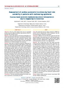
3. Results 3.1. Descriptive Results. Figure 1 compares the skewness of the parameters with and without transformation using natural logarithms. It indicates that the four parameters BR, SDBR, HR, and SDNN need to be log-transformed since they were of skewed distribution and their skewness values largely decreased after performing the log-transformation. Table 3 shows the values (mean ± SD) of the six cardiorespiratory parameters BR, SDBR, HR, SDNN, LF, and HF analyzed in this study for different cohort sets in different genders, age groups, BMI groups, time periods, and sleep stages. The values significantly differed across different groups for all the cohort sets (ANOVA F-test, P < 0.001). 3.2. Multilevel Modeling. In comparison with the F-test, the multilevel regression models enable a more adequate and thorough statistical analysis. With the multilevel Model #1, the estimated coefficients and variances for all the parameters are shown in Table 4. As a result of removing the insignificant variables (tested using the Wald Z-test with P > 0.05) except for the constant intercept and sleep stage variables, the model was optimized. The table indicates that the demographics significantly influenced the cardiorespiratory activity from different aspects. Upon a closer look, it is found that the breathing rate, BR, for the healthy subjects with a higher BMI was significantly higher than the subjects with a lower BMI (0.011 ln-Hz per kg⋅m−2 , P < 0.01) at the baseline of −1.458 ln-Hz, whereas its variation SDBR remained the same. For cardiac activity, the mean heart rate HR of women was

BR

SDBR HR SDNN LF Cardiorespiratory parameter

HF

Original Natural logarithm

Figure 1: Skewness comparison of cardiorespiratory parameters with and without natural logarithm transformation, indicating that BR, SDBR, HR, and SDNN should be log-transformed.

higher than men (0.042 ln-bpm, P < 0.05) at the baseline of 4.221 ln-bpm while its variation SDNN were lower than men (−0.247 ln-ms, P < 0.0001) at the baseline of 4.823 lnms. SDNN were also negatively correlated to subject age (−0.009 ln-ms per y, P < 0.0001) and BMI (−0.025 ln-ms per kg⋅m−2 , P < 0.01). With the spectral analysis of HRV, men had an LF power increased by 0.045 nu (P < 0.05) but a lower HF power of 0.052 nu (P < 0.01) compared with women during bedtime sleep. The HF power slightly decreased along with the increase in age (−0.002 nu per y, P < 0.05). These results are consistent with previous work [18, 61, 62]. Most of the analyzed parameters were found to be timevariant (i.e., they were modulated by time of night) with an exception of breathing rate (Table 4). For instance, the heart rate HR dropped down gradually along with the time progression over the night (−0.0001 ln-bpm per min, P < 0.0001) at the baseline of 4.221 ln-bpm while the variation in heartbeat intervals SDNN increased (0.001 ln-ms per min, P < 0.0001) at the baseline of 4.823 ln-ms, confirming the findings reported previously [63]. This time modulation varied from subject to subject because of the presence of significant variance Ω𝑡 (P < 0.0001), referring to the random time effect. The time was also modulated by some demographic variables (such as age for SDNN and BMI for SDBR, LF, and HF). We note in the table that there appeared to be significant between-subject physiological effects for all parameters (P < 0.0001), measured by the random variances of sleep stage variables. These variances seemed approximately homogeneous across sleep stages for BR and HR but were clearly different for their variations SDBR and SDNN. Figure 2 illustrates an example that compares the parameter values (estimated by multilevel regression based on Model #1) changing along with time between two subjects with different demographics. It shows that the fixed time and demographic

Computational Intelligence and Neuroscience

7

Table 3: Values (mean ± SD) of the six cardiorespiratory parameters in different cohort sets. Cohort set (𝑛 = 165)

Respiratory parameters BR, ln-Hz SDBR, ln-Hz

HR, ln-bpm

Cardiac parameters SDNN, ln-ms LF, nu

HF, nu

Gender Man Woman

−1.20 ± 0.24 −1.22 ± 0.23

−3.67 ± 0.75 −3.81 ± 0.76

4.13 ± 0.15 4.16 ± 0.16

3.74 ± 0.77 3.49 ± 0.71

0.42 ± 0.23 0.39 ± 0.22

0.47 ± 0.23 0.50 ± 0.23

Age Young Middle Elderly

−1.24 ± 0.24 −1.20 ± 0.24 −1.18 ± 0.20

−3.85 ± 0.74 −3.71 ± 0.78 −3.70 ± 0.71

4.11 ± 0.16 4.15 ± 0.16 4.17 ± 0.13

3.94 ± 0.63 3.52 ± 0.69 3.39 ± 0.81

0.36 ± 0.20 0.45 ± 0.23 0.38 ± 0.24

0.56 ± 0.22 0.45 ± 0.23 0.45 ± 0.22

BMI Underweight Normal Overweight

−1.24 ± 0.14 −1.23 ± 0.23 −1.18 ± 0.24

−4.00 ± 0.66 −3.77 ± 0.74 −3.70 ± 0.77

4.11 ± 0.12 4.14 ± 0.16 4.15 ± 0.15

4.01 ± 0.53 3.72 ± 0.73 3.46 ± 0.75

0.36 ± 0.18 0.41 ± 0.22 0.39 ± 0.23

0.56 ± 0.19 0.48 ± 0.23 0.48 ± 0.23

Time of night 0–90 min 90–180 min 180–270 min >270 min

−1.22 ± 0.22 −1.21 ± 0.22 −1.20 ± 0.23 −1.21 ± 0.24

−3.81 ± 0.80 −3.85 ± 0.75 −3.77 ± 0.77 −3.66 ± 0.72

4.16 ± 0.15 4.17 ± 0.15 4.15 ± 0.16 4.12 ± 0.15

3.52 ± 0.73 3.58 ± 0.74 3.61 ± 0.77 3.67 ± 0.75

0.39 ± 0.22 0.42 ± 0.23 0.41 ± 0.23 0.40 ± 0.22

0.50 ± 0.23 0.46 ± 0.23 0.48 ± 0.23 0.49 ± 0.23

Sleep stage Wake REM sleep Light sleep Deep sleep

−1.16 ± 0.23 −1.18 ± 0.22 −1.23 ± 0.23 −1.24 ± 0.23

−3.25 ± 0.62 −3.44 ± 0.52 −3.89 ± 0.73 −4.29 ± 0.71

4.19 ± 0.15 4.15 ± 0.16 4.13 ± 0.15 4.14 ± 0.15

3.61 ± 0.78 3.64 ± 0.76 3.64 ± 0.73 3.45 ± 0.72

0.42 ± 0.24 0.45 ± 0.23 0.40 ± 0.22 0.33 ± 0.21

0.44 ± 0.23 0.42 ± 0.22 0.49 ± 0.23 0.57 ± 0.21

Note: ln, natural logarithm; nu, normalized unit; young, 20–39 y; middle, 40–69 y; elderly, >69 y; underweight, 25 kg⋅m−2 ; light sleep, S1 and S2 stages; deep sleep, S3 and S4 stages. For all the parameters, values between each cohort group were significantly different (𝐹-test, 𝑃 < 0.001) but this may be imprecise since subject demographics, time of night, and sleep stages were possibly not independent.

effects were generally larger than the differences between sleep stages. With the addition of the centering variable to Model #1, we have Model #2 and the estimated regression coefficients after model optimization (Wald Z-test at P < 0.05, for each coefficient) are shown in Table 5. As stated, this model included the between-subject physiological effect at the overnight mean level (i.e., centering effect), resulting in an obvious reduction of the random variance in each sleep stage compared with Model #1. This indicates that regardless of sleep stage the between-subject variability in physiology can be reflected, to a certain degree, by the difference of the mean value over night. Besides, centering the parameter values per subject slightly influenced the time effect in both fixed and random parts. In comparison with Model #1, a lower deviance using Model #2 was obtained for all the parameters (P < 0.0001) as shown in Tables 4 and 5, indicating a better goodness-of-fit on the parameters using the model with the centering variable. Normality of the variances was tested and suggested using the Q-Q plot method for all models. For example, the Q-Q plots of the residual variances Ω𝑒 (in Model #1) for all the parameters are shown in Figure 3, suggesting

that the variances were approximately drawn from a normal distribution. 3.3. Proportion of Variance Explained (PVE). To discover which effects explained the variance and how much each constituted we computed for each cardiorespiratory parameter the PVE for each effect by analyzing the estimated variances of random intercept and residual in a sequence of models (Models A–G in the Appendix). The variance changes in the models with the inclusion of different effects in a specific order are shown in Table 6, based on which the PVE values were obtained in Table 7. Note that the variances explained by sleep stages were not included in PVE. For BR and HR, the between-subject centering effects dominated the variances (55.26% for BR and 77.95% for HR), indicating that the subjects behaved differently with respect to their breathing rate and heart rate at the general mean level throughout the whole night. We also see that the variations in breathing rate and heart rate had a lower centering difference between subjects (with PVE of 26.23% for SDBR and of 39.06% for SDNN) compared with the physiological variability within subjects (with PVE of 61.69% for SDBR and of 40.87% for SDNN). This was also the case for

8

Computational Intelligence and Neuroscience

Table 4: Coefficients and their standard errors (SE) of the optimized multilevel model without the between-subject centering effect (Model #1) for the six cardiorespiratory parameters analyzed in this study. Model coef.

Respiratory parameters BR, ln-Hz

SDBR, ln-Hz

Cardiac parameters HR, ln-bpm

SDNN, ln-ms

LF, nu

HF, nu

Coefficient (SE)

Fixed −1.458 (0.087)

−3.320 (0.032)

4.221 (0.016)

4.823 (0.255)

0.464 (0.014)

0.535 (0.027)

Baseline

Baseline

Baseline

Baseline

Baseline

Baseline

𝛽REM

0.002 (0.008)

NS

−0.205 (0.026)

−0.028 (0.001)

−0.104 (0.027)

0.030 (0.007)

−0.037 (0.007)

𝛽light

−0.035 (0.008)

−0.611 (0.026)

−0.061 (0.001)

−0.052 (0.021)

−0.027 (0.006)

0.039 (0.006)

𝛽deep

−0.044 (0.010)

−0.997 (0.033)

−0.055 (0.001)

−0.249 (0.026)

−0.096 (0.008)

0.106 (0.008)

𝛽0 𝛽wake

−0.009 (0.002)

𝛽𝑎 𝛽𝑔 𝛽𝑏

0.042 (0.021)

−0.247 (0.069)

−0.0001 (0.2e − 4)

0.001 (0.0002)

0.052 (0.017)

0.0004 (0.0001)

−0.0004 (0.0001)

−0.025 (0.011)

0.011 (0.004)

𝛽𝑡

−0.002 (0.001) −0.045 (0.018)

0.001 (0.0004)

−1.0e − 5 (0.3e − 5)

𝛽𝑡𝑎 𝛽𝑡𝑔 −2.8e − 5 (1.3e − 5)

𝛽𝑡𝑏

−1.7e − 5 (0.5e − 5) 1.7e − 5 (0.5e − 5) Coefficient (SE)

Random Ω0 Ωwake

0.030 (0.003)

0.159 (0.018)

0.018 (0.002)

0.224 (0.025)

0.018 (0.002)

0.014 (0.002)

ΩREM

0.029 (0.003)

0.171 (0.020)

0.019 (0.002)

0.280 (0.031)

0.022 (0.002)

0.018 (0.002)

Ωlight

0.030 (0.003)

0.219 (0.024)

0.020 (0.002)

0.256 (0.028)

0.019 (0.002)

0.017 (0.002)

Ωdeep Ω𝑡

0.031 (0.003)

0.257 (0.029)

0.020 (0.002)

0.324 (0.036)

0.020 (0.002)

0.017 (0.002)

1.2e − 7 (0.1e − 7)

6.6e − 7 (0.8e − 7)

3.5e − 8 (0.4e − 8)

7.2e − 7 (0.8e − 7)

5.0e − 8 (0.6e − 8)

4.6e − 8 (0.5e − 8)

0.019 (0.0001)

0.290 (0.001)

0.003 (0.00001)

0.230 (0.001)

0.033 (0.0001)

0.033 (0.0001)

−150487

217253

−398075

186380

−75029

−74306

Residual Ω𝑒 Deviance

Note: ln, natural logarithm; nu, normalized unit; NS, not significant. The statistically significant effects (Wald 𝑍-test, 𝑃 < 0.05), the fixed constant intercept 𝛽0 , and sleep stage intercepts 𝛽𝑠 are presented.

LF and HF powers in the spectral domain of HRV as shown in Table 7. As a result, the overall between-subject variability had more influence on breathing rate (PVE of 66.58%) and heart rate (PVE of 86.25%) while less on their variations (PVE of 37.94%, 58.66%, 33.62%, and 35.13% for SDBR, SDNN, LF, and HF, resp.) compared with the overall within-subject variability. In general, the variances explained by the effects in physiology between subjects (including the effect at the overnight mean level and random effect) and within subjects accounted for 83.83–97.16% of the total variance for different cardiorespiratory parameters. Specifically, a relative larger percentage (13.7%) of the demographic effect can be found on SDNN compared with the other parameters. The PVE of between-subject physiological variability (in the random part) ranged from 2.27% to 7.62% depending on the parameters. For the time effect, the PVE in the fixed part (0.01–1.32%) reflecting the linear changes of parameters over time within subjects was smaller than in the random part (1.58–2.74%) with the indication of

different changes over time between subjects. In general, the time effect accounted for much less of the total variance than most other effects. Finally, although the cross-interactions existed between time and demographics for BR, SDNN, LF, and HF, the proportion of variance they explained was very small ( 0.05) and the variances presented in the table were all statistically significant (Wald 𝑍-test, 𝑃 < 0.01).

Computational Intelligence and Neuroscience

13

Table 7: Proportion of variance explained (PVE, %) accounted for by different effects for the six cardiorespiratory parameters analyzed in this study. Effect

Respiratory parameters

Cardiac parameters SDNN LF

BR

SDBR

HR

HF

Demographic effect

3.55%

1.37%

3.36%

13.69%

0.63%

3.70%

Centering (physiological) effect

55.26%

26.23%

77.95%

39.06%

28.63%

26.41%

2.00%

1.87%

1.58%

3.91%

3.49%

3.44%

Overall between-subject effect

Between-subject time effect

2.74%

2.72%

2.67%

Between-subject physiological effect

5.03%

7.62%

2.27%

0.01%

0.37%

1.32%

0.42%

0.16%

0.14%

33.39%

61.69%

12.43%

40.87%

65.04%

64.54%

0.02%

Ne

Ne

0.06%

0.18%

0.19%

Overall within-subject effect Within-subject time effect Within-subject physiological effect Cross-interaction effect Demographic-related time effect

Note: ln, natural logarithm; Ne, no effect. For each cardiorespiratory parameter, the sum of PVEs from all the effects is 100%, representing the total variance for that parameter. The centering effect reflected some between-subject physiological variability (at the overnight mean level) that was assumed to be independent of sleep stage composition over the entire night.

Table 8: Comparison of sleep staging results (wake/REM sleep/light sleep/deep sleep) using different schemes in correcting the cardiorespiratory parameters.

Overall performance Accuracy, % Kappa coefficient Sleep stage composition (percentage) Wake, % REM sleep, % Light sleep, % Deep sleep, %

PSG

BS

CS1

CS2

CS3

— —

55.8 ± 9.8 0.19 ± 0.10

60.4 ± 8.8 0.29 ± 0.11

62.9 ± 7.8 0.35 ± 0.09

83.5 ± 14.4 0.72 ± 0.23

19.8 ± 12.5 14.0 ± 5.6 53.4 ± 10.7 12.8 ± 7.2

19.9 ± 14.4 0.7 ± 1.0 74.7 ± 15.1 4.7 ± 5.6

18.4 ± 4.9 2.4 ± 2.0 73.5 ± 8.1 5.7 ± 5.2

20.6 ± 6.4 3.0 ± 1.7 71.0 ± 8.2 5.4 ± 4.0

19.7 ± 10.7 10.5 ± 7.8 59.9 ± 12.0 9.9 ± 7.6

Note: BS, baseline with original parameter values without correction; CS1, with correction by fixed effects; CS2, with correction by fixed effects and betweensubject random effects; CS3, with correction by fixed effects and within-subject random effect (model residual). For CS2 and CS3, results were obtained when assuming the sleep stages were known, which was usually not the case in practice. For accuracy and Kappa coefficient, significance of difference between using each correction scheme and BS was confirmed with a paired (two-sided) Wilcoxon signed-rank test, all at 𝑃 < 0.00001.

better correct the parameters. Compared to the parameters analyzed in this study, exploring new parameters with smaller random variances (i.e., those that are less influenced by the between- or within-subject physiological variability) or additional information in separating sleep stages may improve the sleep staging variability performance. Nevertheless, we argue that the performance of cardiorespiratory-based sleep staging will always be limited unless the between- and/or within-subject random variances are successfully explained and corrected.

Appendix The sequence of models constructed to compute the PVE values for different effects is described in as follows. (i) The first model is the model with solely the constant and random intercepts as well as the fixed sleep stage dependent variables. This baseline model can be written as

Model A: A A + ∑𝛽𝑠A 𝑠𝑖𝑗 + 𝑒0𝑖𝑗 , 𝑦𝑖𝑗 = 𝛽0A + 𝜇0𝑗 𝑠

with

A 𝜇0𝑗

(A.1) ∼

𝑁 (0, ΩA0 ) ,

A 𝑒0𝑖𝑗

∼

𝑁 (0, ΩA𝑒 ) ,

where 𝑠 = wake, REM, light, and deep sleep and the total variance Ωtotal consists of variance in two levels: the betweensubject variance ΩA0 at the subject level and the within-subject (residual) variance ΩA𝑒 at the time/epoch level. The percentage of the total variance taken by ΩA0 , called intragroup correlation coefficient (ICC) 𝜌 [43, 59], is computed by 𝜌=

ΩA0 ΩA0 = . Ωtotal (ΩA𝑒 + ΩA0 )

(A.2)

(ii) Let us then consider the model with fixed time effect at the first level

14

Computational Intelligence and Neuroscience Model B:

Model D: D D + ∑𝛽𝑠D 𝑠𝑖𝑗 + 𝛽𝑡D time𝑖𝑗 + 𝛽𝑐D 𝑦𝑗 + 𝑒0𝑖𝑗 𝑦𝑖𝑗 = 𝛽0D + 𝜇0𝑗

B 𝐵 𝑦𝑖𝑗 = 𝛽0B + 𝜇0𝑗 + ∑𝛽𝑠B 𝑠𝑖𝑗 + 𝛽𝑡𝐵 time𝑖𝑗 + 𝑒0𝑖𝑗 ,

𝑠

𝑠

(A.3)

B B ∼ 𝑁 (0, ΩB0 ) , 𝑒0𝑖𝑗 ∼ 𝑁 (0, ΩB𝑒 ) . with 𝜇0𝑗

For the variance analysis of the time variable, instead of using the original time stamps mentioned before (i.e., time𝑖𝑗 = 𝑖/2), we use the shifted (centered) values computed as the original time minus the mean value of the median time over all subjects. This is because, for a longitudinal multilevel analysis, time is an occasional variable within subjects and it usually suffices a linear trend for the measurements since it thus would explain part of total variance in both levels [43]. Actually, with and without shifting the occasion measures do result in equivalent models with exactly the same model coefficients (including residual) and deviance except for the variance estimates of random effects. The variance estimates obtained by shifting the time values are considered to be more accurate and realistic [43]. To quantify the PVE constituted by the fixed time effect, we exploit the relative variance reduction of the baseline model in the two levels 𝑅12 and 𝑅22 , such that PVEtime fixed = = =

(1 − 𝜌) 𝑅12 𝜌 (ΩA𝑒

−

+ 𝜌𝑅22

ΩB𝑒 )

ΩA𝑒

+

(1 −

𝜌) (ΩA0 ΩA0

[(ΩA𝑒 − ΩB𝑒 ) + (ΩA0 − ΩB0 )] Ωtotal

−

(A.4)

𝑦𝑖𝑗 =

from which the corresponding PVE is computed such that C D [(ΩC𝑒 − ΩD 𝑒 ) + (Ω0 − Ω0 )]

PVEcenter =

Ωtotal

.

(A.8)

(v) For the inclusion with cross-interactions that express the demographic-related time effects, the model is as follows: Model E: E E + ∑𝛽𝑠E 𝑠𝑖𝑗 + 𝛽𝑡E time𝑖𝑗 + 𝛽𝑐E 𝑦𝑗 + 𝑒0𝑖𝑗 𝑦𝑖𝑗 = 𝛽0E + 𝜇0𝑗 𝑠

+ 𝛽𝑎E age𝑗 + 𝛽𝑔E gender𝑗 + 𝛽𝑏E BMI𝑗 E E + 𝛽𝑡𝑎 (time × age)𝑖𝑗 + 𝛽𝑡𝑔 (time × gender)𝑖𝑗

(A.9)

E + 𝛽𝑡𝑏 (time × BMI)𝑖𝑗 ,

and the proportion of cross-interaction variance is E D E [(ΩD 𝑒 − Ω𝑒 ) + (Ω0 − Ω0 )]

Ωtotal

.

(A.10)

In addition to the fixed part, we consider the random part of some effects. (vi) The model with additional random time effect is as follows: Model F:

+ ∑𝛽𝑠C 𝑠𝑖𝑗 𝑠

+ 𝛽𝑔C gender𝑗 with

D D D with 𝜇0𝑗 ∼ 𝑁 (0, ΩD 0 ) , 𝑒0𝑖𝑗 ∼ 𝑁 (0, Ω𝑒 ) ,

PVEcross =

.

Model C: C + 𝜇0𝑗

(A.7)

E E with 𝜇0𝑗 ∼ 𝑁 (0, ΩE0 ) , 𝑒0𝑖𝑗 ∼ 𝑁 (0, ΩE𝑒 ) ,

ΩB0 )

Now we consider the subject-level fixed effects. (iii) The model including demographic variables is as follows:

𝛽0C

+ 𝛽𝑎D age𝑗 + 𝛽𝑔D gender𝑗 + 𝛽𝑏D BMI𝑗

+ 𝛽𝑡C time𝑖𝑗

C + 𝑒0𝑖𝑗

+ 𝛽𝑏C BMI𝑗

C 𝜇0𝑗

∼

F 𝑦𝑖𝑗 = 𝛽0F + 𝜇0𝑗 + ∑𝛽𝑠F 𝑠𝑖𝑗 + (𝛽𝑡F + 𝜇𝑡𝑗F ) time𝑖𝑗 + 𝛽𝑐F 𝑦𝑗

+ 𝛽𝑎C age𝑗

𝑠

(A.5)

𝑁 (0, ΩC0 ) ,

C 𝑒0𝑖𝑗

∼

[(ΩB𝑒 − ΩC𝑒 ) + (ΩB0 − ΩC0 )] Ωtotal

.

+ 𝛽𝑎F age𝑗

+ 𝛽𝑔F gender𝑗 + 𝛽𝑏F BMI𝑗

F F + 𝛽𝑡𝑎 (time × age)𝑖𝑗 + 𝛽𝑡𝑔 (time × gender)𝑖𝑗

𝑁 (0, ΩC𝑒 ) .

F + 𝛽𝑡𝑏

Similarly, the PVE explained by the between-subject demographic variables can be computed by PVEdemographic =

F + 𝑒0𝑖𝑗

(A.6)

The demographic variables only explain the variability between subjects, so the variance change at the epoch level should be approximately zero (ΩB𝑒 − ΩC𝑒 = 0). (iv) Further, Model D is the model with the inclusion of between-subject centering effect (expressing the physiological difference between subjects at the overnight mean level), given by

(A.11)

(time × BMI)𝑖𝑗 ,

F 𝜇0𝑗 ΩF0 0 F with [ F ] ∼ 𝑁 ([ ] , [ F ]) , 𝑒0𝑖𝑗 ∼ 𝑁 (0, ΩF𝑒 ) . 0 𝜇𝑡𝑗 Ω𝑡

The computation of the PVE accounted for by the random time effect can be accordingly obtained by PVEtime random =

[(ΩE𝑒 − ΩF𝑒 ) + (ΩE0 − ΩF0 )] Ωtotal

.

(A.12)

(vii) Afterwards, the model with random effects for different sleep stages (expressing the between-subject physiological variability associated with each sleep stage in random part) is then expressed as

Computational Intelligence and Neuroscience

15

References

Model G: G 𝑦𝑖𝑗 = 𝛽0G + 𝜇0𝑗 + ∑ (𝛽𝑠G + 𝜇𝑠𝑗G ) 𝑠𝑖𝑗 + (𝛽𝑡G + 𝜇𝑡𝑗G ) time𝑖𝑗 𝑠

G + 𝛽𝑐G 𝑦𝑗 + 𝑒0𝑖𝑗 + 𝛽𝑎G age𝑗 + 𝛽𝑔G gender𝑗 + 𝛽𝑏G BMI𝑗 G G + 𝛽𝑡𝑎 (time × age)𝑖𝑗 + 𝛽𝑡𝑔 (time × gender)𝑖𝑗

(A.13)

G + 𝛽𝑡𝑏 (time × BMI)𝑖𝑗 , G 𝜇0𝑗 ΩG 0 0 [ [ G] ] [ G] G G ] ∼ 𝑁 ([ ] 𝜇 0 , with [ Ω ] [ 𝑡𝑗 [ 𝑡 ]) , 𝑒0𝑖𝑗 ∼ 𝑁 (0, Ω𝑒 ) . [ ] G [0] [ΩG [ 𝜇𝑠𝑗 ] 𝑠 ]

In this model, the random variance ΩG 𝑠 not only explains the variance in ΩF0 and ΩF𝑒 , but also reflects some variance of the random time effect ΩF𝑡 . Therefore, the proportion of variance contained in ΩG 𝑠 to the total variance is as follows: PVEbetw subj random =

F G F G [(ΩF𝑒 − ΩG 𝑒 ) + (Ω0 − Ω0 ) + (Ω𝑡 − Ω𝑡 )]

Ωtotal

(A.14) .

Then the PVE of the random time effect to the total variance should be corrected to PVEtime random =

[(ΩE𝑒 − ΩF𝑒 ) + (ΩE0 − ΩF0 ) − (ΩF𝑡 − ΩG 𝑡 )] Ωtotal

.

(A.15)

(viii) Finally, the remaining residual variance is assumed to only associate with the physiological variability within subjects and its proportion can be obtained such that PVEwithin subj random =

ΩG 𝑒 . Ωtotal

(A.16)

Note that all these models are optimized by only keeping the variables that do not statistically equal zero.

Conflict of Interests No conflict of interests, financial or otherwise, is declared by the authors.

Acknowledgments The authors gratefully thank Tine Smits and Dr. Sam Jelfs from Philips Research for their insightful comments and proofreading of the paper. The SIESTA database used in the present study was supported by the European Commission, DG XII (Project no. Biomed-2 BMH4-CT97-2040) between Sep. 1997 and Aug. 2000.

[1] C. A. Kushida, M. R. Littner, T. Morgenthaler et al., “Practice parameters for the indications for polysomnography and related procedures: an update for 2005,” Sleep, vol. 28, no. 4, pp. 499– 521, 2005. [2] E. A. Rechtschaffen and A. Kales, A Manual of Standardized Terminology, Techniques and Scoring System for Sleep Stages of Human Subjects, National Institutes of Health, Washington, DC, USA, 1968. [3] C. Iber, S. Ancoli-Israel, A. L. Chesson, and S. F. Quan, The AASM Manual for the Scoring of Sleep and Associated Events: Rules, Terminology & Technical Specifications, American Academy of Sleep Medicine, Westchester, Ill, USA, 2007. [4] J. Hedner, D. P. White, A. Malhotra et al., “Sleep staging based on autonomic signals: a multi-center validation study,” Journal of Clinical Sleep Medicine, vol. 7, no. 3, pp. 301–306, 2011. [5] J. M. Kortelainen, M. O. Mendez, A. M. Bianchi, M. Matteucci, and S. Cerutti, “Sleep staging based on signals acquired through bed sensor,” IEEE Transactions on Information Technology in Biomedicine, vol. 14, no. 3, pp. 776–785, 2010. [6] S. J. Redmond, P. de Chazal, C. O’Brien, S. Ryan, W. T. McNicholas, and C. Heneghan, “Sleep staging using cardiorespiratory signals,” Somnologie, vol. 11, no. 4, pp. 245–256, 2007. [7] A. Roebuck, V. Monasterio, E. Gederi et al., “A review of signals used in sleep analysis,” Physiological Measurement, vol. 35, no. 1, pp. R1–R57, 2014. [8] T. Watanabe and K. Watanabe, “Noncontact method for sleep stage estimation,” IEEE Transactions on Biomedical Engineering, vol. 51, no. 10, pp. 1735–1748, 2004. [9] N. J. Douglas, D. P. White, C. K. Pickett, J. V. Weil, and C. W. Zwillich, “Respiration during sleep in normal man,” Thorax, vol. 37, no. 11, pp. 840–844, 1982. [10] D. W. Hudgel, R. J. Martin, B. Johnson, and P. Hill, “Mechanics of the respiratory system and breathing pattern during sleep in normal humans,” Journal of Applied Physiology: Respiratory, Environmental and Exercise Physiology, vol. 56, no. 1, pp. 133– 137, 1984. [11] X. Long, P. Fonseca, R. M. Aarts, R. Haakma, and J. Foussier, “Modeling cardiorespiratory interaction during human sleep with complex networks,” Applied Physics Letters, vol. 105, no. 20, Article ID 203701, 2014. [12] F. Snyder, J. A. Hobson, D. F. Morrison, and F. Goldfrank, “Changes in respiration, heart rate, and systolic blood pressure in human sleep,” Journal of Applied Physiology, vol. 19, pp. 417– 422, 1964. [13] J. Trinder, J. Kleiman, M. Carrington et al., “Autonomic activity during human sleep as a function of time and sleep stage,” Journal of Sleep Research, vol. 10, no. 4, pp. 253–264, 2001. [14] Task Force of the European Society of Cardiology and the North American Society of Pacing and Electrophysiology, “Heart rate variability: standards of measurement, physiological interpretation and clinical use,” Circulation, vol. 93, no. 5, pp. 1043–1065, 1996. [15] J. P. Saul, R. F. Rea, D. L. Eckberg, R. D. Berger, and R. J. Cohen, “Heart rate and muscle sympathetic nerve variability during reflex changes of autonomic activity,” The American Journal of Physiology—Heart and Circulatory Physiology, vol. 258, no. 3, pp. H713–H721, 1990. [16] E. A. Phillipson, “Control of breathing during sleep,” The American Review of Respiratory Disease, vol. 118, no. 5, pp. 909– 939, 1978.

16 [17] M. I. Polkey, M. Green, and J. Moxham, “Measurement of respiratory muscle strength,” Thorax, vol. 50, no. 11, pp. 1131– 1135, 1995. [18] G. Brandenberger, A. U. Viola, J. Ehrhart et al., “Age-related changes in cardiac autonomic control during sleep,” Journal of Sleep Research, vol. 12, no. 3, pp. 173–180, 2003. [19] H. R. Peterson, M. Rothschild, C. R. Weinberg, R. D. Fell, K. R. McLeish, and M. A. Pfeifer, “Body fat and the activity of the autonomic nervous system,” The New England Journal of Medicine, vol. 318, no. 17, pp. 1077–1083, 1988. [20] A. Y. Schumann, R. P. Bartsch, T. Penzel, P. C. Ivanov, and J. W. Kantelhardt, “Aging effects on cardiac and respiratory dynamics in healthy subjects across sleep stages,” Sleep, vol. 33, no. 7, pp. 943–955, 2010. [21] R. L. Horner, “Autonomic consequences of arousal from sleep: mechanisms and implications,” Sleep, vol. 19, pp. S193–S195, 1996. [22] A. Sgoifo, C. Coe, S. Parmigiani, and J. Koolhaas, “Individual differences in behavior and physiology: causes and consequences,” Neuroscience and Biobehavioral Reviews, vol. 29, no. 1, pp. 1–2, 2005. [23] D. P. White, J. V. Weil, and C. W. Zwillich, “Metabolic rate and breathing during sleep,” Journal of Applied Physiology, vol. 59, no. 2, pp. 384–391, 1985. [24] H. J. Burgess, A. L. Holmes, and D. Dawson, “The relationship between slow-wave activity, body temperature, and cardiac activity during nighttime sleep,” Sleep, vol. 24, no. 3, pp. 343– 349, 2001. [25] H. J. Burgess, T. Sletten, N. Savic, S. S. Gilbert, and D. Dawson, “Effects of bright light and melatonin on sleep propensity, temperature, and cardiac activity at night,” Journal of Applied Physiology, vol. 91, no. 3, pp. 1214–1222, 2001. [26] N. Carter, R. Henderson, S. Lal, M. Hart, S. Booth, and S. Hunyor, “Cardiovascular and autonomic response to environmental noise during sleep in night shift workers,” Sleep, vol. 25, no. 4, pp. 457–464, 2002. [27] A. Muzet, “Environmental noise, sleep and health,” Sleep Medicine Reviews, vol. 11, no. 2, pp. 135–142, 2007. [28] M. H. Bonnet and D. L. Arand, “Heart rate variability: sleep stage, time of night, and arousal influences,” Electroencephalography and Clinical Neurophysiology, vol. 102, no. 5, pp. 390–396, 1997. ˚ [29] T. Akerstedt, A. Knutsson, P. Westerholm, T. Theorell, L. Alfredsson, and G. Kecklund, “Sleep disturbances, work stress and work hours: a cross-sectional study,” Journal of Psychosomatic Research, vol. 53, no. 3, pp. 741–748, 2002. [30] P. Grossman, F. H. Wilhelm, and M. Spoerle, “Respiratory sinus arrhythmia, cardiac vagal control, and daily activity,” The American Journal of Physiology—Heart and Circulatory Physiology, vol. 287, no. 2, pp. H728–H734, 2004. [31] M. Hall, R. Vasko, D. Buysse et al., “Acute stress affects heart rate variability during sleep,” Psychosomatic Medicine, vol. 66, no. 1, pp. 56–62, 2004. [32] G. Kl¨osch, B. Kemp, T. Penzel et al., “The SIESTA project polygraphic and clinical database,” IEEE Engineering in Medicine and Biology Magazine, vol. 20, no. 3, pp. 51–57, 2001. [33] J. A. Van Alste and T. S. Schilder, “Removal of base-line wander and power-line interference from the ECG by an efficient FIR filter with a reduced number of taps,” IEEE Transactions on Biomedical Engineering, vol. 32, no. 12, pp. 1052–1060, 1985.

Computational Intelligence and Neuroscience [34] P. Fonseca, R. M. Aarts, J. Foussier, and X. Long, “A novel low-complexity post-processing algorithm for precise QRS localization,” SpringerPlus, vol. 3, article 376, 2014. [35] A. M. Bianchi, L. Mainardi, E. Petrucci, M. G. Signorini, M. Mainardi, and S. Cerutti, “Time-variant power spectrum analysis for the detection of transient episodes in HRV signal,” IEEE Transactions on Biomedical Engineering, vol. 40, no. 2, pp. 136–144, 1993. [36] A. Boardman, F. S. Schlindwein, A. P. Rocha, and A. Leite, “A study on the optimum order of autoregressive models for heart rate variability,” Physiological Measurement, vol. 23, no. 2, pp. 325–336, 2002. [37] X. Long, J. Yang, T. Weysen et al., “Measuring dissimilarity between respiratory effort signals based on uniform scaling for sleep staging,” Physiological Measurement, vol. 35, no. 12, pp. 2529–2542, 2014. [38] R. L. Burr, “Interpretation of normalized spectral heart rate variability indices in sleep research: a critical review,” Sleep, vol. 30, no. 7, pp. 913–919, 2007. [39] A. Domingues, T. Paiva, and J. M. Sanches, “Hypnogram and sleep parameter computation from activity and cardiovascular data,” IEEE Transactions on Biomedical Engineering, vol. 61, no. 6, pp. 1711–1719, 2014. [40] X. Long, J. Foussier, P. Fonseca, R. Haakma, and R. M. Aarts, “Analyzing respiratory effort amplitude for automated sleep stage classification,” Biomedical Signal Processing and Control, vol. 14, pp. 197–205, 2014. [41] S. J. Redmond and C. Heneghan, “Cardiorespiratory-based sleep staging in subjects with obstructive sleep apnea,” IEEE Transactions on Biomedical Engineering, vol. 53, no. 3, pp. 485– 496, 2006. [42] E. Bagiella, R. P. Sloan, and D. F. Heitjan, “Mixed-effects models in psychophysiology,” Psychophysiology, vol. 37, no. 1, pp. 13–20, 2000. [43] J. J. Hox, Multilevel Analysis: Techniques and Applications, Routledge, London, UK, 2010. [44] P. E. Wainwright, S. T. Leatherdale, and J. A. Dubin, “Advantages of mixed effects models over traditional ANOVA models in developmental studies: a worked example in a mouse model of fetal alcohol syndrome,” Developmental Psychobiology, vol. 49, no. 7, pp. 664–674, 2007. [45] S. Raudenbush and A. S. Bryk, “A hierarchical model for studying school effects,” Sociology of Education, vol. 59, no. 1, pp. 1–17, 1986. [46] M. van de Pol and J. Wright, “A simple method for distinguishing within- versus between-subject effects using mixed models,” Animal Behaviour, vol. 77, no. 3, pp. 753–758, 2009. [47] H. Goldstein, W. Browne, and J. Rasbash, “Multilevel modelling of medical data,” Statistics in Medicine, vol. 21, no. 21, pp. 3291– 3315, 2002. [48] C. S. McCrae, J. P. H. Mcnamara, M. A. Rowe et al., “Sleep and affect in older adults: using multilevel modeling to examine daily associations,” Journal of Sleep Research, vol. 17, no. 1, pp. 42–53, 2008. [49] E. J. Mezick, K. A. Matthews, M. Hall et al., “Intra-individual variability in sleep duration and fragmentation: associations with stress,” Psychoneuroendocrinology, vol. 34, no. 9, pp. 1346– 1354, 2009. [50] P. D. Bliese, N. J. Wesensten, and T. J. Balkin, “Age and individual variability in performance during sleep restriction,” Journal of Sleep Research, vol. 15, no. 4, pp. 376–385, 2006.

Computational Intelligence and Neuroscience [51] G. E. Silva, J. L. Goodwin, D. L. Sherrill et al., “Relationship between reported and measured sleep times: the Sleep Heart Health Study (SHHS),” Journal of Clinical Sleep Medicine, vol. 3, no. 6, pp. 622–630, 2007. [52] H. P. Van Dongen, N. L. Rogers, and D. F. Dinges, “Sleep debt: theoretical and empirical issues,” Sleep and Biological Rhythms, vol. 1, no. 1, pp. 5–13, 2003. [53] A. P. J. van Eekelen, J. H. Houtveen, and G. A. Kerkhof, “Circadian variation in base rate measures of cardiac autonomic activity,” European Journal of Applied Physiology, vol. 93, no. 1-2, pp. 39–46, 2004. [54] J. M. A. Graham, S. A. Janssen, H. Vos, and H. M. E. Miedema, “Habitual traffic noise at home reduces cardiac parasympathetic tone during sleep,” International Journal of Psychophysiology, vol. 72, no. 2, pp. 179–186, 2009. [55] X. Long, R. Haakma, R. M. Aarts, P. Fonseca, and J. Foussier, “Between-laboratory and demographic effects on heart rate and its variability during sleep,” in Proceedings of the Workshop on Smart Healthcare and Healing Environments, Springer, Eindhoven, The Netherlands, 2014. [56] S. S. Shapiro, M. B. Wilk, and H. J. Chen, “A comparative study of various tests for normality,” Journal of the American Statistical Association, vol. 63, pp. 1343–1372, 1968. [57] L. J. Cronbach, “Research in classrooms and schools: formulation of questions, designs and analysis,” Occasional Paper, Stanford Evaluation Consortium, 1976. [58] J. Rasbash, F. Steele, W. J. Browne, and H. Goldstein, A User’s Guide to MLwiN, Centre for Multilevel Modelling, University of Bristol, Bristol, UK, 2009. [59] S. W. Raudenbush and A. S. Bryk, Hierarchical Linear Models, Sage, Thousand Oaks, Calif, USA, 2002. [60] J. A. Cohen, “A coefficient of agreement for nominal scales,” Educational and Psychological Measurement, vol. 20, pp. 37–46, 1960. [61] S. Elsenbruch, M. J. Harnish, and W. C. Orr, “Heart rate variability during waking and sleep in healthy males and females,” Sleep, vol. 22, no. 8, pp. 1067–1071, 1999. [62] S. M. Ryan, A. L. Goldberger, S. M. Pincus, J. Mietus, and L. A. Lipsitz, “Gender- and age-related differences in heart rate dynamics: are women more complex than men?” Journal of the American College of Cardiology, vol. 24, no. 7, pp. 1700–1707, 1994. [63] H. J. Burgess, J. Trinder, Y. Kim, and D. Luke, “Sleep and circadian influences on cardiac autonomic nervous system activity,” The American Journal of Physiology—Heart and Circulatory Physiology, vol. 273, no. 4, pp. H1761–H1768, 1997. [64] A. L. Holmes, H. J. Burgess, and D. Dawson, “Effects of sleep pressure on endogenous cardiac autonomic activity and body temperature,” Journal of Applied Physiology, vol. 92, no. 6, pp. 2578–2584, 2002. [65] V. K. Somers, M. E. Dyken, M. P. Clary, and F. M. Abboud, “Sympathetic neural mechanisms in obstructive sleep apnea,” The Journal of Clinical Investigation, vol. 96, no. 4, pp. 1897–1904, 1995.

17

Journal of

Advances in

Industrial Engineering

Multimedia

Hindawi Publishing Corporation http://www.hindawi.com

The Scientific World Journal Volume 2014

Hindawi Publishing Corporation http://www.hindawi.com

Volume 2014

Applied Computational Intelligence and Soft Computing

International Journal of

Distributed Sensor Networks Hindawi Publishing Corporation http://www.hindawi.com

Volume 2014

Hindawi Publishing Corporation http://www.hindawi.com

Volume 2014

Hindawi Publishing Corporation http://www.hindawi.com

Volume 2014

Advances in

Fuzzy Systems Modelling & Simulation in Engineering Hindawi Publishing Corporation http://www.hindawi.com

Hindawi Publishing Corporation http://www.hindawi.com

Volume 2014

Volume 2014

Submit your manuscripts at http://www.hindawi.com

Journal of

Computer Networks and Communications

 Advances in 

Artificial Intelligence Hindawi Publishing Corporation http://www.hindawi.com

Hindawi Publishing Corporation http://www.hindawi.com

Volume 2014

International Journal of

Biomedical Imaging

Volume 2014

Advances in

Artificial Neural Systems

International Journal of

Computer Engineering

Computer Games Technology

Hindawi Publishing Corporation http://www.hindawi.com

Hindawi Publishing Corporation http://www.hindawi.com

Advances in

Volume 2014

Advances in

Software Engineering Volume 2014

Hindawi Publishing Corporation http://www.hindawi.com

Volume 2014

Hindawi Publishing Corporation http://www.hindawi.com

Volume 2014

Hindawi Publishing Corporation http://www.hindawi.com

Volume 2014

International Journal of

Reconfigurable Computing

Robotics Hindawi Publishing Corporation http://www.hindawi.com

Computational Intelligence and Neuroscience

Advances in

Human-Computer Interaction

Journal of

Volume 2014

Hindawi Publishing Corporation http://www.hindawi.com

Volume 2014

Hindawi Publishing Corporation http://www.hindawi.com

Journal of

Electrical and Computer Engineering Volume 2014

Hindawi Publishing Corporation http://www.hindawi.com

Volume 2014

Hindawi Publishing Corporation http://www.hindawi.com

Volume 2014