Effects of point-spread function on calibration and radiometric accuracy of CCD camera Hong Du and Kenneth J. Voss
The point-spread function 共PSF兲 of a camera can seriously affect the accuracy of radiometric calibration and measurement. We found that the PSF can produce a 3.7% difference between the apparent measured radiance of two plaques of different sizes with the same illumination. This difference can be removed by deconvolution with the measured PSF. To determine the PSF, many images of a collimated beam from a He–Ne laser are averaged. Since our optical system is focused at infinity, it should focus this source to a single pixel. Although the measured PSF is very sharp, dropping 4 and 6 orders of magnitude and 8 and 100 pixels away from the point source, respectively, we show that the effect of the PSF as far as 100 pixels away cannot be ignored without introducing an appreciable error to the calibration. We believe that the PSF should be taken into account in all optical systems to obtain accurate radiometric measurements. © 2004 Optical Society of America OCIS codes: 110.4100, 120.5630, 070.2590, 100.3020.
1. Introduction
CCD cameras have been widely used to simultaneously obtain an array of digitized radiometric values with high linearity and precision. One can easily interpret the image as the per-pixel distribution of radiance, but as pointed out by Huang1 and Townshend,2 a substantial portion of the signal of each pixel comes from surrounding areas. Indeed, this is true for many optical systems. For example, it has been estimated that less than half of the signal recorded by Landsat’s first Multispectral Scanner System comes from the area imaged by the pixel itself.1,3 This means the real radiance of a pixel should be regarded as a function of the signals of an area surrounding it, instead of just the pixel. Qiu et al.4 further reported that the characterization of the point spread function 共PSF兲 well away from the center is necessary to achieve accurate radiometric assessment in the presence of moderate-to-highcontrast scenes. The PSF of an optical system is the consequence of many factors, including the system optics, the sensor, and the electronics5 and will cer-
The authors are with the Department of Physics, University of Miami, 1320 Campo Sano Drive, Coral Gables, Florida 33124. H. Du’s e-mail address is
[email protected]. Received 10 July 2003; revised manuscript received 16 October 2003; accepted 22 October 2003. 0003-6935兾04兾030665-06$15.00兾0 © 2004 Optical Society of America
tainly get worse if the optical system is not well focused or is dirty.6 Because of the impact of the PSF on image acquisition, including satellite remote sensing, it is very important to characterize and deconvolute the PSF far away from the central point in order to obtain accurate radiometric values. In this paper, we will introduce a new method of measuring the PSF of a CCD camera system with a laser beam. The effect of the PSF is demonstrated by the simulation of radiance sources of different sizes and also by a calibration experiment. It is clearly shown that the PSF should be taken into account in any calibration and interpretation of data obtained with an imaging system. 2. Measuring and Modeling the PSF
Many techniques have been employed to obtain the PSF. Taking images of a point source such as a bright star6,7 if the camera is outside the atmosphere or a very small bright object8 is the most direct means of measuring the PSF. A line source can be used to measure the line spread function and obtain the PSF indirectly.9 The PSF can also be computed by use of the measured bidirectional reflectance distribution function of the scan mirror and the bidirectional scatter distribution function of key optical elements in the camera system.4 It is also possible to determine the PSF from images of apertures of arbitrary shapes.10 But in this paper we focus on the direct measurement with an expanded laser beam. Be20 January 2004 兾 Vol. 43, No. 3 兾 APPLIED OPTICS
665
cause the laser beam is collimated, it can be effectively viewed as a point source placed at infinity. The CCD camera system being studied consists of a 24-mm, f2.5 Tamron 01BB camera lens with nine elements, and an Apogee AP47 CCD camera with a 16-bit analog-to-digital converter. The shortest exposure time is 0.01 s, and the exposure time can be varied in 0.01-s increments. The CCD camera contains a Marconi CCD47-10 backthinned CCD sensor array with 1056 ⫻ 1027, 13 m ⫻ 13 m pixels; however we will use 2 ⫻ 2 binning and truncate the array to 512 ⫻ 512. The lens is focused as closely as possible to infinity, and the pixel angular resolution is approximately 0.057 deg兾pixel. A 2-log neutral density filter is inserted in front of the camera lens, and a 3.2-mm-diameter aperture is placed behind the lens to act as a fixed aperture stop. A 0.95-mW HeNe laser is set 5 m from the camera, pointing directly at the camera lens so that the laser appears as a point source in the center of a CCD pixel. A beam expander expands the laser beam to cover the entire entrance aperture of the camera. The experiment is performed in a dark room to avoid stray light. A 4-log neutral-density filter is used to attenuate the laser beam so that the focused laser will not saturate the central pixel on the CCD. With this setup, the laser generates a spot on the CCD sensor with the strongest signal occupying just 3– 4 pixels. Markham11 and Cracknell12 found it infeasible to directly measure a two-dimensional PSF because of the difficulty in producing a point source of significant intensity. In our case the problem is the opposite. The 0.95-mW He–Ne laser without attenuation is far too strong even for the shortest exposure time. The real challenge is that outside of the few bright pixels, the signal level is low. In order to maximize the signal-to-noise ratio 共SNR兲, the exposure time is set to obtain the maximum counts in the central bright spot without blooming. Longer exposure times, with blooming of the central pixel, can improve the SNR of the darker pixels, but care must be taken to avoid using the bloom affected area. The bright spot has digital counts 共DC兲 on the order of 104; the area immediately surrounding the bright spot consists of pixels with 102 DC or lower. The remaining pixels are very dark; their signals are soon surpassed by readout noise just a few pixels away from the bright spot. Thus we need to average many images to increase the SNR. To simplify the characterization of the PSF, we assume that the PSF is radially symmetric across the sensor. The simplified PSF is then written as PSF共r兲, where r is the radial distance between the image of the point source and the pixel. The brightest pixel is selected as the origin 共r ⫽ 0兲. At r ⬎ 0, PSF共r兲 is the radial average of all the pixels that are r pixels away from the brightest pixel. Radial averaging also helps increase the SNR, since it averages the values of 2rdr pixels. Thus as r increases and the signal decreases, the number of pixels averaged increases as r increases. In practice, r is rounded into multiples of 0.5. For the same PSF共r兲 measured 666
APPLIED OPTICS 兾 Vol. 43, No. 3 兾 20 January 2004
Fig. 1. PSF measured at exposures of 0.02 and 0.08 s 共radial average scaled to 0.01 s of exposure time兲. Also shown is the fitted PSF with C1 ⫽ 40 and C2 ⫽ 0.3 by use of Eq. 共3兲.
with different exposure times, the measurements are scaled to a fixed exposure time. We define the digital counts scaled to the equivalent of 0.01-s exposure time as the scaled digital counts 共SDC兲. The scaled radial average, or the measured PSF共r兲, is then in units of SDC. In our experiment, the camera is exposed for 0.01– 0.09 s in 0.01-s increments. For each exposure, an associated dark image is taken immediately after the light image, the procedure is repeated ten times, and the images are averaged together. A software program automatically operates the camera and records the raw data onto the hard drive without manual intervention. Figure 1 shows the scaled radial average obtained with exposure times of 0.02 and 0.08 s. Figure 1 clearly shows that most of the data points are very noisy. This is caused by the nature of the CCD image sensor. Because most pixels receive very little signal, two sensor-related characteristics, the readout noise and the Poisson statistics, significantly degrade the SNR. For a specific exposure time, the standard deviations of the radial average caused by readout noise and Poisson statistics are d共r兲 ⬇
D 共N2rdr兲 1兾2
(1)
and
冋
M共r兲 P共r兲 ⬇ N2rdr
册
1兾2
,
(2)
respectively, where D is the standard deviation of the readout noise of 1 pixel in DC, N is the number of images used to obtain the radial average, and M共r兲 is the radial average in DC. When the noises at different exposure times are scaled to the equivalent noise of a 0.01 exposure, they have the units of SDC. The standard deviation D of the CCD camera is found to be about 13 DC by analyzing the dark images of the CCD camera exposed for 0.01 s. The radial average M共r兲 drops sharply as r increases. Based on Eqs. 共1兲
Table 2. Sum of PSF 共Not Normalized兲 versus Summation Limit R
Table 1. First Six Points of Measured and Normalized PSFs
Distance from Point Source in Pixels
Measured PSF Value
Normalized PSF Value
Summation Limit R in Pixels
Sum of PSF
Percent of Total
0.0 1.0 2.0 3.0 4.0 5.0
25555 6231 98.89 21.90 8.111 4.829
0.3965 0.09667 1.534 ⫻ 10⫺3 3.398 ⫻ 10⫺4 1.258 ⫻ 10⫺4 7.492 ⫻ 10⫺5
0 1 2 10 20 50 75 100 120 150 200 230 250 300 350 400 500 600 700 1000
25555 50479 58987 60271 61064 62379 62969 63337 63556 63791 64035 64129 64178 64266 64323 64361 64406 64428 64440 64454
39.6 78.3 91.5 93.5 94.7 96.8 97.7 98.3 98.6 99.0 99.3 99.5 99.6 99.7 99.8 99.86 99.93 99.96 99.98 100
and 共2兲 and the curves shown in Fig. 1, it is found that the major noise source is the readout noise when r ⬎ 2 关d共r兲 ⬎ P共r兲兴. For example, in Fig. 1 the radial average M共10兲 is ⬃1.7 SDC. The standard deviation of the readout noise is d共10兲 ⬇ 0.7 SDC, whereas the standard deviation of the Poisson statistics is P共10兲 ⬇ 0.07 SDC, much smaller than d共10兲. The near field 共r ⱕ 2兲 data points have a much higher SNR, but blooming causes a large difference between the 0.02-s and the 0.08-s radial averages. The PSF共r兲 is chosen to be the scaled radial average of the 0.02-s images for r ⱕ 5, because the SNR is high and blooming does not occur. The first six points of the PSF are listed in Table 1. The rest of the data can be fit with function
P SF共r兲 ⫽
C 1 exp共⫺C 2 冑r兲 r
sum of the readings of all pixels is unity. The expression of this normalization is Pˆ SF共r兲 ⫽
(3)
by adjusting constants C1 and C2. Since the points near the center are experimentally determined and do not use this equation, the singularity of Eq. 共3兲 at the origin is not a problem. Constant C2 is a small positive number, and it determines the shape of PSF. It was found that this function follows the radial average better than other forms of the PSF, such as a Gaussian.1,5 The fitted PSF shown in Fig. 1 uses C1 ⫽ 40 and C2 ⫽ 0.3 and appears a little lower than the measured data points at r ⬎ 100. This is to accommodate the fact that some negative data points are not shown in this graph owing to the logarithmic y axis. 3. Normalization of PSF
Radiometric concepts must be defined in order to normalize the PSF. Suppose there is an incident beam of light filling only the solid angle corresponding to 1 pixel. Ideally this pixel would collect all of the incoming photons in the light beam. The pixel counts would then be proportional to the radiance in that solid angle, if exposure time and pixel area are taken into account. However, in reality, the PSF causes some of the photons to be spread into other pixels or even outside the CCD array. So the sum of all the photons distributed according to the PSF rather than just the reading of 1 pixel should be proportional to the radiance. We normalize the PSF such that the
P SF共r兲 R
R
兺 兺
.
(4)
P SF关共 x 2 ⫹ y 2兲 1兾2兴
x⫽⫺R y⫽⫺R
In this equation, the summation is from ⫺R to R, where R should be as large as possible in order to include all the energy spread by the PSF. Although Fig. 1 shows that the PSF drops 6 orders of magnitude at a distance of 100 pixels, it will produce an unacceptable error if the summation limits are set to 100. Experimentally, the whole CCD array is under appreciable influence of the PSF if a large bright object is imaged, even if the image of the bright object is on the edge of the CCD sensor or out of the field of view. This means R should be larger than 512. To demonstrate the effect of the summation limit, we use the fitted PSF and list the summations of the PSF with different R values in Table 2. It is seen from the table that the summation limit R should be larger than 230 pixels in order to include more than 99.5% of all the photons. If the limit R is set to 100 pixels, only 98.3% of all the photons are taken into account. This missing 1.7% will interfere with the calibration and radiometric interpretation of images when it is not accounted for. In this paper, the summation limit is set to 1000, and the normalized PSF is given by Pˆ SF共r ⬎ 5兲 ⫽
6.206 ⫻ 10 ⫺4 exp共⫺0.3 冑r兲 . r
(5)
The first six points of the normalized PSF are also shown in Table 1. It is interesting to see in this table that less than half of the energy actually ends 20 January 2004 兾 Vol. 43, No. 3 兾 APPLIED OPTICS
667
up in the central pixel; about 60% of the energy corresponding to the incident light is spread elsewhere. This means that if a star is sampled by this camera, the simple interpretation of the reading of just 1 pixel as the radiometric measurement will under estimate the intensity by 60% percent. It is found that the measurement of PSF共0兲 is sensitive to the focus of the camera and the alignment of the laser point source relative to the center of a CCD pixel, so care must be taken to keep this alignment error as low as possible. In the presence of an alignment error, only the first few points of the PSF are affected.
4. Validation of the Large-Angle PSF
Since the data away from the center has a very low SNR, it is necessary to raise the digital counts in that area. For example if the central pixel is as bright as possible 共for example 51,110 DC兲, the average DC 200 pixels away is only 0.0057 DC. Although this weak signal does bias the readout noise and can be determined by averaging a large number of pixels, the poor SNR can threaten the credibility of these values. Raising the signal level by increasing the intensity of the point source is not possible, because of the limited dynamic range of the CCD. Expanding the solid angle of the source can raise the counts at large angles without saturating the central pixels by superimposing many PSFs. If the image of the source is a circular area with a radius of 6 pixels, the pointspread-photon counts at larger angles will be 62 ⬇ 113 times stronger than that due to a single pixel. The 0.0057 DC discussed above can be raised to ⬃0.64 DC, which is more acceptable. Notice that the light source does not have to be perfectly uniform, because the counts at large angles are proportional to the total flux of the light source; thus the shape of the PSF at large angles is preserved. To create this source, the 0.95-mW expanded He–Ne laser beam aimed directly at the CCD camera is intercepted by semitransparent tape. The semitransparent tape diffuses the collimated laser beam and creates a light source ⬃2.8 cm in diameter. This light source is strongest in the forward direction. Both the 2-log and 4-log neutral-density filters, discussed previously, are removed. Stray light is carefully blocked with a black cloth in order to keep unwanted light from contaminating the weak signal. The distance between the area source and the camera is ⬃1 m, so the full angle of the light source viewed by the camera is approximately 1.6 deg. Figure 2 shows the radial average of 96 images of this light source with an exposure time of 2 s. It is seen that the curve is much cleaner at large angles than that shown in Fig. 1. A PSF using Eq. 共3兲 with C2 ⫽ 0.3 and C1 ⫽ 3600, is also shown in Fig. 2. It can be seen that the fitted curve is very close to the measured data at r ⬎ 70. Since the constant C2 determines the shape of the PSF at large angles, Fig. 2 can be viewed as confirmation of the fitted PSF in Fig. 1. 668
APPLIED OPTICS 兾 Vol. 43, No. 3 兾 20 January 2004
Fig. 2. Radial average of a circular area source generated by diffusing the expanded He–Ne laser beam. Also shown is a fit to the PSF with C1 ⫽ 3600 and C2 ⫽ 0.3.
5. Calibration, Radiometric Interpretation, and the PSF
As sharp as the PSF is, the large angle effects of the PSF can not be ignored without appreciable radiometric consequences. Assume a perfect optical system. In this case square plaques with the same reflectance and illumination but of different sizes can be imaged, and the apparent radiance of the plaques will be constant 共assume unity兲. In a real optical system, images obtained are actually the convolution of the square plaques with the normalized PSF of the system. Table 3 shows the calculated brightness of the centers of the square plaques of different sizes affected by the PSF of the CCD camera discussed above. We can see that the center of a 3 ⫻ 3 pixel square plaque is almost 10% less than unity, a 51 ⫻ 51 plaque is 4.5% less than unity, and a 251 ⫻ 251 square plaque is still 1.1% less than unity. Even if the image occupies all of the CCD pixels, the reading at the center of the square will still be less than unity, because some energy is spread out of the CCD array. This variation 共approximately 3.4% between the 51and 251-pixel square plaques兲 is a significant error in a radiometric calibration and raises a serious problem if the images are interpreted directly as radiance. The obvious answer to this problem is that the correct
Table 3. Calculated Center Brightness versus Size of Square Plaques of Unit Radiance
Brightness at the Center of Plaque
Length of Square Plaques in Pixels
0.3965 0.8968 0.9282 0.9372 0.9546 0.9704 0.9793 0.9849 0.9887 0.9913 0.9947 0.9966
1 3 11 21 51 101 151 201 251 301 401 501
radiometric values must be the deconvoluted results with the corresponding PSF of the camera system. We carried out a deconvolution based on the Fast Fourier Transform and Inverse Fast Fourier Transform techniques.6 The Fourier Transform 共FT兲 of the convoluted camera image, FT关image共x, y兲兴, equals the product of the FTs of the normalized PSF, FT关Pˆ SF共x, y兲兴, and the radiance field, FT关L共x, y兲兴. Therefore the radiance field may be deconvoluted from the image by taking the Inverse Fourier Transform IFT of the ratio FT关image共x, y兲兾FT关Pˆ SF共x, y兲兴, namely, L共 x, y兲 ⫽ IFT兵FT关image共 x, y兲兴兾FT关Pˆ SF共 x, y兲兴其.
(6)
In practice, the radiance field, the image, and the PSF are all expressed as M ⫻ M matrices, where Pˆ SF共x, y兲 is related to Pˆ SF共r兲 through P SF共 x, y兲 ⫽ P SF(兵关mod共 x ⫹ M兾2, M兲 ⫺ M兾2兴 2 ⫹ 关mod共 y ⫹ M兾2, M兲 ⫺ M兾2兴 2其 1兾2), (7) where the origin of r is set at the 共0, 0兲 element of the M ⫻ M matrix. To reduce the aliasing across the boundary, the digitized 512 ⫻ 512 image can be expanded into a 1024 ⫻ 1024 matrix, with the digitized image located at its center. In our experiment the pixels corresponding to the padding elements are illuminated only by the light spread from the central light source; therefore the padding elements are filled with the convolution of the digitized image with Pˆ SF共x, y兲. To experimentally examine the effect of the PSF on the calibration of our CCD camera system, we use two Labsphere-certified 共North Sutton, New Hampshire兲 Spectralon reflectance standards; a square plaque 25.4 ⫻ 25.4 cm, and a round 5.08-cm-diameter plaque. These two plaques have the same nominal 99% reflectance at visible wavelengths and were illuminated by a 1000-W FEL lamp at a distance of 50 cm in a dark room. The CCD camera was approximately 1 m from the plaque and viewed the plaque 45 degrees to the plaque surface normal. To the CCD camera, the big plaque is a trapezoid approximately 315 pixels tall and 220 pixels wide, whereas the small plaque is an ellipse approximately 60 pixels tall and 40 pixels wide. Under the same illumination condition, an average of 9 ⫻ 9 pixels in the center of the large plaque is 38487 ⫾ 175 DC, whereas for the small plaque it is 37072 ⫾ 242 DC, a 3.7% difference. If the images of both the large and the small plaques are deconvoluted with the normalized PSF of the CCD camera, the average of 9 ⫻ 9 pixels in the center of the large plaque is 39034 ⫾ 591 DC, whereas for the small plaque it is 38941 ⫾ 542 DC. The deconvolution process tends to increase the noise level in the image, because the deconvolution tends to enhance the contrast of both the signal and the noise.10 But the average of repeated experiments is quite consistent. By comparing 10 deconvoluted images of both the large and small plaques, we found the aver-
ages of the 9 ⫻ 9 pixel areas in these images were 39097 ⫾ 53 DC for the large plaque and 38977 ⫾ 20 DC for the small plaque. The difference of the averages is now reduced to 0.3%, with the large plaque slightly brighter. We see that not only is the difference reduced but also the absolute values of both the small and the large plaques are raised by 5.1% and 1.6%, respectively. To make sure that the large plaque is only slightly brighter than the small plaque, a well-baffled single-lens radiometer, with a field of view of 0.08°, was used to measure the brightness of each plaque. Internal baffling was also used to expose only a 2° field of view of the plaque to the radiometer’s aperture. The radiometer’s internal baffling and simple optics restrict its optical system’s full PSF within this 2° limit. This radiometer measures a radiance 0.24% larger for the large plaque than the small one. This confirms that the large plaque is only slightly brighter than the small plaque, as shown by our deconvolution results. Just as removing the effect of the PSF is essential for precise calibration, careful characterization of the camera’s PSF is equally essential, because the accuracy of the PSF will affect the accuracy of the calibration coefficients. Each optical system will have a characteristic PSF that must be measured precisely. This conclusion about the calibration should be extended to all radiometric interpretation of images, since the calibration image is just a special case of imagery. Many researchers have noticed that the PSF tends to smooth or blur images with high contrast,1,8 and the remotely sensed images are badly offset by bright clouds.4 This is by no means a surprise, because the PSF tends to spread energy everywhere and lowers the contrast. Images of small structures such as stars, sharp spectral lines, dark spots, and the boundaries of bright objects and dark objects will be seriously affected by the PSF. This makes the per-pixel interpretation erroneous in two ways. First, it will decrease the signal in bright pixels. Second, dark pixels can be increased by a considerable bias; the larger the image of the source is, the worse the bias is. The bias can be dominant when the signal itself is small. Even though the PSF may drop several orders at larger angles, a large source can make an appreciable difference on other pixels. For example, consider a 101 ⫻ 101 pixel square of unit radiance. By doing a convolution, the PSF used in this paper will contribute about 0.19, 0.026, 0.018, and 0.01 extra radiance 1, 3, 8, and 20 pixels, respectively, away from the edge of the square. On the other hand, the radiance of the square itself appears to be 0.79, 0.95, 0.96, and 0.97 instead of unity at 0, 3, 8, and 20 pixels, respectively, from the edge into the plaque. It is clear that the only way to remove the artificial radiance variation is to deconvolute the image with the system PSF and return the radiance of the plaque back to the true value. 6. Conclusion
We have successfully measured and modeled the PSF of a CCD camera and used the PSF function to dem20 January 2004 兾 Vol. 43, No. 3 兾 APPLIED OPTICS
669
onstrate that only the deconvoluted image can be interpreted as the correct radiometric image. A deconvolution technique based on Fast Fourier Transform兾Inverse Fast Fourier Transform is described. The deconvolution with the normalized PSF successfully removed the artificial 3.7% calibration difference between a large plaque and a small plaque. We see that the characterization of the PSF, including large angle values, is an indispensable part of radiometric measurement utilizing a camera system. The PSF is intrinsic to all optical systems. The images obtained with the camera are imprinted with the influence of the PSF from light sources inside as well as outside the field of view. The influence of the PSF is conspicuous where there is high contrast; however, the theoretically correct radiometric interpretation of the image is complete only if the PSF is accounted for. This research was supported by National Aeronautics and Space Administration grant NAS 5-31363. References 1. C. Huang, J. R. G. Townshend, S. Liang, S. N. V. Kalluri, and R. S. DeFries, “Impact of sensor’s point spread function on land cover characterization: assessment and deconvolution,” Remote Sens. Environ. 80, 203–212 共2002兲. 2. J. R. G. Townshend, C. Huang, S. N. Kalluri, R. S. DeFries, S. Liang, and K. Yang, “Beware of per-pixel characterization of land cover,” Int. J. Remote Sens. 21, 839 – 843 共2000兲.
670
APPLIED OPTICS 兾 Vol. 43, No. 3 兾 20 January 2004
3. J. R. G. Townshend, “The spatial resolving power of earth resources satellites,” Prog. Phys. Geog. 5, 32–55 共1981兲. 4. S. Qiu, G. Godden, X. Wang, and B. Guenther, “Satellite–Earth remote sensor scatter effects on Earth scene radiometric accuracy,” Metrologia 37, 411– 414 共2000兲. 5. R. A. Schowengerdt, Remote Sensing 共Academic, San Diego, Calif., 1997兲. 6. H. Li, M. S. Robinson, and S. Murchie, “Preliminary remediation of scattered light in NEAR MSI images,” Icarus 155, 244 – 252 共2002兲. 7. S. Murchie, M. Robinson, S. E. Hawkins III, A. Harch, P. Helfenstein, P. Thomas, K. Peacock, W. Owen, G. Heyler, P. Murphy, E. H. Darlington, A. Keeney, R. Gold, B. Clark, N. Izenberg, J. F. Bell III, W. Merline, and J. Veverka, “Inflight calibration of the NEAR Multispectral Imager,” Icarus 140, 66 –91 共1999兲. 8. J. Lehr, J. B. Sibarita, and J. M. Chassery, “Image restoration in x-ray microscopy: PSF determination and biological applications,” IEEE Trans. Image Process. 7, 258 –263 共1998兲. 9. J. Zandhuis, D. Pycock, S. Quigley, and P. Webb, “Sub-pixel nonparametric PSF estimation for image enhancement,” IEE Proceedings. Vision Image Signal Process. 144, 285–292 共1997兲. 10. N. H. Nakashima and A. W. S. Johnson, “Measuring the PSF from aperture images of arbitrary shape–an algorithm,” Ultramicroscopy 94, 135–148 共2003兲. 11. B. L. Markham, “The Landsat sensors’ spatial responses,” IEEE Trans. Geosci. Remote Sens. 23, 864 – 875 共1985兲. 12. A. P. Cracknell, “Synergy in remote sensing–what’s in a pixel,” Int. J. Remote Sens. 19, 2025–2047 共1998兲.