Efficient Approximation Algorithms for Repairing Inconsistent Databases Andrei Lopatenko Google & Free University of Bozen–Bolzano
[email protected]
Abstract We consider the problem of repairing a database that is inconsistent wrt a set of integrity constraints by updating numerical values. In particular, we concentrate on denial integrity constraints with numerical built-in predicates. So far research in this context has concentrated in computational complexity analysis. In this paper we focus on efficient approximation algorithms to obtain a database repair and we present an algorithm that runs in O(n log n) wrt the size of the database. Our experimental evaluations show that even for large databases an approximate repair of the database can be computed efficiently despite the fact that the exact problem is computationally intractable. Finally, we show that our results can also be applied to database repairs obtained by a minimal number of tuple deletions.
1. Introduction When merging different database instances in a data exchange setting, the resulting database may be inconsistent wrt a set of integrity constraints. Two techniques have been used to deal with inconsistent databases: data cleaning [19, 17] and consistent query answering (CQA) [3]. While data cleaning results in a new consistent database, CQA keeps the inconsistent database as is and considers the ICs at query time to return only the so called “consistent answers”. In [4] techniques from CQA were modified to perform data cleaning, i.e. for finding a unique repair of the database. In this paper we aim at providing optimized algorithms for those modified techniques. A repair of a database can be obtained by deletions and insertions of whole tuples as well as by updating attributes, generally under the assumption that the repair should be “as close as possible” to the inconsistent
Loreto Bravo Carleton University & University of Edinburgh
[email protected]
database. This closeness can be interpreted in many different ways such as minimal number of changes, minimal set of changes under set inclusion and minimal numerical distance (refer to [3] for a survey and references of notions considered in CQA). Example 1.1 Consider a database that classifies different types of papers and their environmental “friendliness”. Each tuple has the ID of the paper, if it is environmentally friendly (EF ), the percentage of Recycled Content (P RC) and if the bleaching process was Chlorine Free (CF ). EF and CF can take values 1 or 0 and P CR is a positive value smaller than 100. A paper is environmentally friendly, i.e. EF = 1, only if the percentage of recycled content is higher or equal to 50% and the bleaching process is chlorine free. The following database is inconsistent wrt this constraint. We add a column in order to label the different tuples. D: Paper ID EF PRC CF B1 C2 E3
1 1 1
40 20 70
0 1 1
t1 t2 t3
Tuples t1 and t2 do not satisfy the constraint. A repair obtained by deleting a minimal number of tuples, would leave only t3 in the database. An alternative approach is to modify the values of some attributes in a minimal way in order to restore consistency. For example, we can solve the inconsistency of the second tuple by changing the value of EF from 1 to 0. Less information is lost when we update attributes. Attribute-update repairs, i.e repairs obtained by updating numerical values that minimize the numerical distance from the original database have been considered before in [21, 22, 4, 6]. This approach is of particular interest for database applications, like census, demographic, financial, and experimental data, that contain quantitative data usually associated to nominal or
qualitative data, e.g. number of children associated to a household identification code (or address); or measurements associated to a sample identification code. This databases may contain semantic constraints. For example, a census form for a particular household may be considered incorrect if the number of children exceeds 20; or if the age of a parent is less than 10. These restrictions can be expressed with denial integrity constraints, that prevent some attributes from taking certain combinations of values [11]. Inconsistencies in numerical data can be resolved by changing individual attribute values, while keeping values in the keys, e.g. without changing the household code, the number of children is decreased considering the admissible values. The optimization problem of finding the minimum distance from an attribute-update repair wrt IC to a given input instance is MAXSNP -hard [4]. By transforming this problem into a minimum weight set cover problem, a repair can be calculated by using approximation algorithms such as the greedy [10] and layer algorithms [13, Chapter 3]. Since the running time of the greedy algorithm is O(n3 ), it is not efficient enough for real databases where the database can have one million or more tuples. In this paper, we introduce a variation of the greedy algorithm that runs in O(n2 log n) in the general case and in O(n log n) under the assumption that a tuple can be involved in a number of inconsistencies that is bounded by a constant. This assumption is valid in most practical cases where a tuple is generally not involved in many inconsistencies. We experiment with – and compare the performance of – the greedy and layer algorithm and their modified versions. We show that the modified greedy algorithm runs faster than the greedy algorithm, and that in its turn, the greedy algorithm runs faster than the layer and modified layer algorithm. We also show that the approximations obtained with the greedy algorithms are better than the ones of the layer algorithms. Finally, we also consider repairs obtained by a minimal number of deletions, i.e. tuple-deletion repairs, and we show that they can also be obtained as attribute-update repairs. This implies that we can also use the modified-greedy algorithm to compute tupledeletion repairs. The paper is structured as follows. Section 2 introduces definitions. Sections 3 describes the transformation of the problem of obtaining attribute-update repairs to the MWSCP, introduces a modified version of the MWSC greedy algorithm and gives a running time analysis of it. Section 4 shows some experimental results that compare the performance of the greedy and layer algorithm and their modified versions. Section 5
shows how to transform the tuple-deletion repair problem into the attribute-update repair problem. Finally Section 6 presents some conclusions.
2. Preliminaries Consider a relational schema Σ = (U, R∪B, A), with domain U that includes Z,1 R a set of database predicates, B a set of built-in predicates, and A a set of attributes. For R ∈ R, AR is a subset of A associated to R. A database instance is a finite collection D of database tuples, i.e. of ground atoms P (¯ c), with P ∈ R and c¯ a tuple of constants in U such that |¯ c| = |AR |. There is a set F ⊆ A of all the flexible attributes, those that take values in Z and are allowed to be modified. Attributes outside F are called hard. F need not contain all the numerical attributes, that is we may also have hard numerical attributes. We assume that each relations R ∈ R has a primary key KR , KR ⊆ AR . K is the set of key constraints. We assume that K is satisfied by the initial instance D, denoted D |= K. It also holds F ∩ KR = ∅, i.e. values in key attributes cannot be updated. In addition, there may be a separate set of flexible ICs IC that may be violated, and it is the job of a repair to restore consistency wrt them (while still satisfying K). A linear denial constraint [14] has the form ∀¯ x¬(A1 ∧ . . . ∧ Am ), where the Ai are database atoms (i.e. with predicate in R), or built-in atoms of the form xθc, where x is a variable, c is a constant and θ ∈ {=, 6=, , ≤, ≥}, x = y or x 6= y. We will usually replace ∧ by commas in denials. We denote by AB (ic) the attributes in built-ins in a constraint ic. A set of linear denials IC is local if: (a) Attributes participating in equality atoms or joins are all hard attributes; (b) For each ic ∈ IC, (AB (ic) ∩ F) 6= ∅; (c) No attribute A appears in IC both in comparisons of the form A < c1 and A > c2 .2 A linear denial constraint ic is said to be local if the set {ic} is local. Local constraints have the property that by doing local fixes, no new inconsistencies will be generated, and there will always exist a repair [4]. Locality is a sufficient, but not necessary condition for existence of repairs. For a tuple k¯ of values for the key KR of relation R ¯ R, D) denotes the unique tuple in an instance D, t¯(k, ¯ To ¯ t in relation R in instance D whose key value is k. each attribute A ∈ F a fixed numerical weight αA is assigned. 1 With
simple denial constraints, numbers can be restricted to, e.g. N or {0, 1}. 2 To check condition (c), x ≤ c, x ≥ c, x 6= c have to be expressed using , e.g. x ≤ c by x < c + 1.
Definition 2.1 [4] For instances D and D 0 over schema Σ with the same set val (KR ) of tuples of key values for each relation R ∈ R and a distance function Dist, the ∆-distance between the databases is X ¯ R, D)), π (t¯(k, ¯ R, D0 ))) ∆(D, D 0 ) = αA Dist(πA (t¯(k, A R∈R,A∈F
¯ k∈val(K R)
where πA is the projection on attribute A. The distance function Dist should increase monotonically over the absolute values of the differences between values and all the results that follow are valid for any such distance. For example, it can be the “city distance” L1 (the sum of absolute differences) or the “euclidian distance” L2 (the sum of the square of differences). The type of distance to use will depend on the type of data stored in the databases. For simplicity in the examples we will assume L1 -distance. The coefficients αA can be chosen in many ways depending on the relevance of the attribute, the actual distribution of the data, or a compensation of different scales of measurement. Definition 2.2 [4] For an instance D, a set of flexible attributes F, a set of key dependencies K, such that D |= K, and a set of flexible ICs IC: A repair candidate for D wrt IC is an instance D 0 such that: (a) D0 has the same schema and domain as D; (b) for every R ∈ ¯ R, D)) = R, A ∈ AR r F and k¯ ∈ val (KR ), πA (t¯(k, 0 0 0 ¯ ¯ πA (t(k, R, D )); (c) D |= K; and (d) D |= IC. A repair for D is a repair candidate D 0 that minimizes the distance ∆(D, D0 ) over all the instances that satisfy (a)–(d). Finally, Rep At (D, IC) is the set of repairs of D wrt IC. 0
Intuitively, D is a repair if it has the same schema as D, does not modify the values in the hard attributes of D, satisfies the constraints and is as close as possible to D. Example 2.3 (example 1.1 continued ) R = {Paper }, A = {ID, EF , PRC , CF }, KPaper = {ID}, F = {EF , 1 1 PRC , CF }, with weights α ¯ = (1, 20 , 2 ), resp. The constraints over environmentally friendly papers can be expressed as ic 1 : ∀xyzw¬(P aper(x, y, z, w) ∧ y > 0 ∧ z < 50) and ic 2 : ∀xyzw¬(P aper(x, y, z, w) ∧ y > 0 ∧ w < 1). The first two tuples of D do not satisfy the constraints. Since we want to repair the database by making the smallest possible modifications, we consider as possible repairs for t1 : t11 = P aper(B1, 0, 40, 0)3 or t21 = P aper(B1, 3 The attributes that are changed wrt the original tuple are in bold.
1, 50, 1), and for t2 : t12 = P aper(C2, 0, 20, 1) or t22 = P aper(C2, 1, 50, 1). Then, there are four natural candidate repairs D1 = {t11 , t12 , t3 }, D2 = {t21 , t12 , t3 }, D3 = {t11 , t22 , t3 } and D4 = {t21 , t22 , t3 }. The respective distances are: ∆(D, D1 ) = 1 + 1 = 2, ∆(D, D2 ) = 1 1 1 20 × 10 + 2 × 1 + 1 = 2, ∆(D, D3 ) = 1 + ( 20 × 30) = 3 1 1 1 and ∆(D, D4 ) = ( 20 × 10 + 2 × 1) + ( 20 × 30) = 2.5. Since D1 and D2 minimize the distance, they are the only repairs for D wrt the constraint: Therefore, the two repairs of the database are: D1 : Paper ID EF PRC CF
D2 :
Paper
B1 C2 E3
0 0 1
40 20 70
0 1 1
t11 t12 t3
ID B1 C2 E3
EF 1 0 1
PRC 50 20 70
CF 1 1 1
t21 t12 t3
Definition 2.4 [4] A set I of database tuples from D is a violation set for ic ∈ IC if I 6|= ic, and for every I 0 $ I, I 0 |= ic. Let I(D, ic) = {I|I is a violation set for ic} and I(D, ic, t) = {I|I ∈ I(D, ic) and t ∈ I}. The degree of inconsistency of a tuple t is Deg(t, IC) = |{I|I ∈ I(D, ic, t), ic ∈ IC}| and the degree of inconsistency of a database D is Deg(D, IC) = M ax{Deg(t, IC)|t ∈ D}. A violation set I for ic is a minimal set of tuples that simultaneously participate in the violation of ic. The degree of inconsistency of a tuple is the number of violation sets that contain it. Example 2.5 (example 2.3 continued) Let us add to our database a table Pub that stores the ID of a publication (e.g. magazine) the ID of the paper used (PID) and its number of pages (Pag ). The primary key for this table is ID and the only flexible attribute is Pag 1 . with αPag = 10 Pub
ID 235 112 100
PID B1 B1 E3
Pag 45 30 80
p1 p2 p3
The publisher has a requirement that publications of more than 40 pages should use paper that contains at least 70% of recycled paper, i.e. ic 3 : ∀xyzuvw¬(P ub(x, y, z) ∧ P aper(y, u, v, w) ∧ z > 40 ∧ v < 70). Then the violation sets for each integrity constraints are: I(D, ic 1 ) = {{t1 }, {t2 }}, I(D, ic 2 ) = {{t1 }} and I(D, ic 3 ) = {{t1 , p1 }}. Note that {ic 1 , ic 2 , ic 3 } is a set of local constraints.
Definition 2.6 Given an instance D and ICs IC, a local fix for t ∈ D, is a tuple t0 with: (a) the same values for the hard attributes as t; (b) S(t, t0 ) := {(I, ic) | ic ∈ IC, I ∈ I(D, ic, t) and ((I r {t}) ∪ {t0 }) |= ic} 6= ∅; and (c) there is no tuple t00 that simultaneously satisfies (a), S(t, t00 ) = S(t, t0 ), modifies the same attributes as t0 and ∆({t}, {t00 }) ≤ ∆({t}, {t0 }), where ∆ denotes the distance function. A mono-local fix is a local fix that modifies only one attribute. S(t, t0 ) contains the violation sets that include t and are solved changing t by t0 . A local fix t0 solves at least one inconsistency and minimizes the distance to t. In [4] it was proven that if D 0 is a repair D wrt IC then ¯ R, D0 ) is for every relation R and every key k¯ in it, t¯(k, ¯ ¯ equal to t¯(k, R, D) or it is a local fix of t¯(k, R, D) wrt to IC. Here, instead of using local fixes, we will show we can concentrate in mono-local fixes. This can be done since any local fix can be seen as a combination of mono-local fixes. Proposition 2.7 Given a tuple t, a local integrity constraint ic and a flexible attribute A such that A ∈ AB (ic), there is a unique mono-local fix t0 that modifies attribute A. Definition 2.8 shows how to obtain the mono-local fix of tuple t that modifies attribute A and solves an inconsistency wrt ic. Definition 2.8 Given a local constraint ic, a tuple t and an attribute A ∈ AB (ic), the tuple MLF (t, ic, A) is obtain by: (1) replacing every ≤ and ≥ in ic by < and >, (2) If ic contains (a) A < c1 , . . . , A < cn then MLF (t, ic, A) is a tuple obtained from t by replacing attribute A by M in{c1, . . . , cn }. (b) A > c1 , . . . , A > cn then MLF (t, ic, A) is a tuple obtained from t by replacing attribute A by M ax{c1 , . . . , cn }. Proposition 2.9 For a database D, a local constraint ic, a tuple t and an attribute A ∈ AB (ic). If I(D, ic, t) 6= ∅, then MLF (t, ic, A) is the unique monolocal fix of t wrt ic for attribute A. Example 2.10 (example 2.3 continued) All the possible local fixes for t1 are t11 = MLF (t1 , IC1 , EF ) = MLF (t1 , IC2 , EF ) = P aper(B1, 0, 40, 0), t21 = P aper(B1, 1, 50, 1), t31 = MLF (t1 , IC1 , PRC ) = Paper (B1, 1, 50, 0) and t41 = MLF (t1 , IC2 , CF ) = Paper (B1, 1, 40, 1). t21 is a local fix but not a monolocal fix since it modifies two attributes. The violation sets solved with each mono-local fix are: S(t1 , t11 ) = S(t1 , t21 ) = {({t1 }, ic 1 ), ({t1 }, ic 2 )}, S(t1 , t31 ) = {({t1 }, ic 1 )} and S(t1 , t41 ) = {({t1 }, ic 2 )}.
3. Attribute-Update Repairs For a fixed set of linear denials IC, the optimization problem of finding the minimum distance from a repair wrt IC to a given input instance is MAXSNP-hard and therefore cannot be uniformly approximated within arbitrarily small constant factors (unless P = NP) [4]. By restricting to a set of local denial constraints the problem is still MAXSNP-hard but can we can transformed into an instance of the Minimum Weighted Set Cover Optimization Problem (MWSCP). Given a collection S of subsets of a set U and a positive weight w(Si ) for each Si ∈ S, a set cover C is a subset of S such that every element in U belongs to at least one member of C. The weight of the cover is the sum of the weights of the sets in it. The MWSCP consists in finding a set cover with a minimum weight. Definition 3.1 For a database D and a set IC of local denials, the instance (U, S, w) for theMWSCP, denoted (U, S, w)(D,IC) , where U is the underlying set, S is the set collection, and w is the weight function, is given by: (a) U := I(D, IC). (b) S contains the S(t, t0 ), where t0 is a mono-local fix for a tuple t ∈ D. (c) w(S(t, t0 )) := ∆({t}, {t0 }). This transformation is a slight modification of the one in [4] where t0 could also be local fix that modified more than one attribute. The modification can be done since a local fix can always be constructed as a combination of mono-local fixes [5, Proposition A.3]. In both cases if we find a minimum weight cover C, we could try to construct the repair by replacing each inconsistent tuple t ∈ D by the mono-local fix t0 with S(t, t0 ) ∈ C. If there is more than one mono-local fix for a tuple t then we need to combine the updates in a unique local fix. This can be done easily since in an optimal solution of the MWSCP, if there is more than one mono-local fixes they will modify different attributes (by Proposition 2.7) and therefore we can construct a unique local fix by combining the updates of the different attributes. Definition 3.2 [4] Let C be a cover for instance (U, S, w)(D,IC) of the MWSCP . (a) C ? is obtained from C as follows: For each tuple t with mono-local fixes t1 , . . . , tn , n > 1, such that S(t, ti ) ∈ C, replace ? ? in C all the S(t, ti ) by Sna single S(t, t ), where t is ? such that S(t, t ) = i=1 S(t, ti ). (b) D(C) is the database instance obtained from D by replacing t by t0 if S(t, t0 ) ∈ C ? . Tuple t? always exists and is a local fix of t obtained from the mono-local fixes t1 , . . . , tn by combining the updates associated to each of them.
Example 3.3 (example 2.5 continued) We illustrate the reduction from DFOP to MWSCP . To construct the MWSCP instance we need the mono-local fixes. The mono-local fixes of t1 are t11 = Paper (B1, 0, 40, 0), t21 = Paper (B1, 1, 50, 0), t31 = Paper (B1, 1, 40, 1) and t41 = Paper (B1, 1, 70, 0) with S(t1 , t11 ) = {({t1 }, ic 1 ), ({t1 }, ic 2 )}, S(t1 , t21 ) = {({t1 }, ic 1 )}, S(t1 , t31 ) = {({t1 }, ic 2 )} and S(t1 , t41 ) = {({t1 }, ic 1 ), ({t1 , p1 }, ic 3 )}. The mono-local fixed of t2 are t12 = Paper (C2, 0, 20, 1) and t22 = Paper (C2, 1, 50, 1) with S(t2 , t12 ) = {({t2 }, ic 1 )} and S(t2 , t22 ) = {({t2 }, ic 1 )}. The mono-local fixes of p1 are p11 = Pub(235, B1, 40) with S(p1 , p11 ) = {({t1 , p1 }, ic 3 )}. The MWSCP instance is shown in the table below, where the elements are rows and the sets (e.g. S1 = S(t1 , t11 )), columns. An entry 1 means that the set contains the corresponding element; and a 0, otherwise. Set Local Fix Weight ({t1 }, ic 1 ) ({t1 }, ic 2 ) ({t2 }, ic 1 ) ({t1 , p1 }, ic 3 )
S1 t11 1 1 1 0 0
S2 t21 0.5 1 0 0 0
S3 t31 0.5 0 1 0 0
S4 t41 1.5 1 0 0 1
S5 t12 1 0 0 1 0
S6 t22 1.5 0 0 1 0
S7 p11 1 0 0 0 1
There are three minimal covers, each with weight 3: C1 = {S1 , S5 , S7 } C2 = {S2 , S3 , S5 , S7 } and C3 = {S3 , S4 , S5 }. Since all the mono-local fixes in C1 correspond to different tuples, the repair associated to it can be obtained by directly replacing each tuple by its fix: D(C1 )={t11 , t12 , t3 , p11 , p2 , p3 }. On the other hand, C2 has two mono-local fixes for t1 . In this case we need to combine t21 and t31 into t51 = (B1, 1, 50, 1) producing the repair D(C2 )={t51 , t12 , t3 , p11 , p2 , p3 }. Finally, for C3 we need to combine t31 and t41 into t61 = (B1, 1, 70, 1) producing the repair D(C3 )={t61 , t12 , t3 , p1 , p2 , p3 }. The MWSCP can be approximated in the general case within a logarithmic factor using the greedy algorithm (see Algorithm 1) [16, 10]. The greedy algorithm consists in choosing at each stage the set which contains the largest number of uncovered elements until all the elements are covered [10]. Example 3.4 (example 3.3 continued) In the first iteration we have wef (S1 ) = 0.5, wef (S2 ) = 0.5, wef (S3 ) = 0.5, wef (S4 ) = 0.75, wef (S5 ) = 1, wef (S6 ) = 1.5 and wef (S7 ) = 1. We can choose S1 , S2 , S3 or S4 . If we choose S1 we get C = {S1 }. Now the effective weights are updated to: wef (S1 ) = undefined, wef (S2 ) = undefined, wef (S3 ) = undefined, wef (S4 ) = 1.5, wef (S5 ) = 1, wef (S6 ) = 1.5 and wef (S7 ) = 1. By choosing S5 we get C = {S1 , S5 }. Now the only effective weights that are not undefined are wef (S4 ) = 1.5 and wef (S7 )
= 1. Therefore we choose S7 and now C = {S1 , S5 , S7 }. All the elements are covered so the process stops and {S1 , S5 , S7 } is an approximate cover. In this case C is an optimal cover. Algorithm 1: GreedySC(U, S, w): Set Cover Greedy Approximation Algorithm Input: An instance (U, S, w) of the MWSCP constructed using Definition 3.1 Output: Set cover C C ← ∅, E ← ∅, i ← 0; while While there are non-covered elements (U r E 6= ∅) do foreach s ∈ S do wef (s) ← w(s) |s| ; M ← element in S with smallest wef ; C ← C ∪ {M } ; S ← S r {M } ; E ←E∪S ; foreach s ∈ S do s←srM return C; A cover that is not optimal might contain two monolocal fixes for the same tuple t and attribute A but for different ICs. In this case in order to construct the repair from the cover, we use the mono-local fix with higher weight, since that one will subsume the other one (since the ICs are local). Proposition 3.5 Given a database D and a set of local linear denial ICs IC, the running time of the greedy algorithm for the instance (U, S, w)(D,IC) of the MWSCP is O(n3 ) for n the size of the D. If Deg(D, IC) is bounded by a constant, the running time is O(n2 ). Proof: The cost of updating the weights, choosing the element with smallest weight and updating set E in iteration i is O(|Si |) where Si is the size of S in iteration i. Since one set is deleted in each iteration, O(|Si |)) is O((|S|−i)). The cost of deleting the covered elements from the sets in Si is O(|Si ||M |), i.e. O(|(S − i)||M |). Then, the cost of each iteration is O((|S| − i)(1+|M |)). In the worst case we will have |S| iteration, i.e. all the sets in S will belong to the cover. Therefore P|S| the running time is i=1 ((|S| − i)(1 + |M |)) = (1 + |M |)(|S|2 − |S|(|S| + 1)/2) which is O((1 + |M |)|S|). S is the set of all possible mono-local fixes for a set of inconsistent tuple, therefore |S| is O(n|F|) for n the number of tuples in the database. On the other hand, in the general case M is O(n) since a tuple my be involved in all the inconsistencies of the database. In this case, this would give us a running time of O(n3 ). If
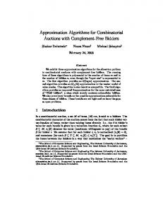
the degree of inconsistency of the database is bounded, then M is also bounded and therefore the algorithm runs in O(n2 ). It is common to find in practice inconsistent databases where the degree of inconsistency is bounded by a small number. For example, in a census databases, where a tuple corresponds to a person and his/her data, each tuple can only be involved in inconsistencies with the tuples representing other members of his/her household [11]. Since the number of members in household can be bounded, by 10 for example, the degree of inconsistency is bounded. Therefore, in most practical cases, we expect the greedy algorithm to run in O(n2 ). Even though the algorithm runs in quadratic time when the degree of inconsistency is bounded, it is still too expensive for large databases (more than one million tuples). This is why we want to modify the greedy algorithm to obtain a more efficient algorithm. The expensive task in the algorithm corresponds to searching for the set with more uncovered elements, i.e. the one with minimum effective weight. We can improve the running time by storing S of the MWSCP in a priority queue P . Each object in the priority queue will contain an inconsistent tuple t, a mono-local fix of it, its weight, and a set of pointers to the elements of the U , i.e. the violation sets. These violation sets will be stored in an array A. Therefore, the modification of the greedy algorithm consists on modifying the data structure that stores the sets and elements, in such a way that we can efficiently search for the set with minimal effective weight. First we will describe how to construct the MWSC problem from the database D and the set of local constraints IC. Algorithm 2 constructs array A containing the violation sets. The violations sets are obtained by rewriting each integrity constraint as a SQL view that is empty if it is being satisfied. Example 3.6 (example 2.3 continued) The violations sets of ic 1 can be retrieved from D by posing the SQL query: SELECT X Y Z W FROM Paper WHERE Y>0 AND Z 25), ∀ID, A, C¬(Client ( ID, A, C), A < 18, C > 50)}. We generated 3 random databases for different sizes with around 30% of tuples involved in inconsistencies and calculated approximation of the repairs of them wrt IC. The results provided for each size correspond to the average of the three results. The first step consisted in comparing the algorithm to determine which gave a better approximation of the database repair problem. The results are shown in Fig-
10000
1x10⁵
1x10⁶
1x10⁷
si ze ofdatabase
Figure 3. Running Time Next, we compared the running time of the MWSCP approximation algorithms. Therefore, we only considered the time of the MWSCP solver component. The results of the experiments are shown in Figure 3. Clearly, the use of a priority queue to store the set of the MWSCP instance increases the performance for large databases for both, the layer and greedy algorithm. More over, the modified greedy algorithm shows to be the most efficient for large databases. The experiments show that the modified-greedy algorithm can be used efficiently to calculate the repairs of database wrt a set of local integrity constraints, even
for large databases. Not only that, but the experiments show that in practice, the modified-greedy algorithms runs faster and gives better approximations than the layer algorithm.
5. Cardinality Repairs So far we have considered repairs that can be obtained by updating values of tuples in the database. Alternatively we could consider repairing inconsistencies by deleting tuples. The “minimality” of the repairing process can be captured by either minimizing the number of tuples (cardinality semantics) to be deleted or by deleting only sets of tuples that are minimal under set inclusion (set semantics). In the context of CQA, the set semantics for tuple deletions and also for tuple deletions and insertions [1, 9, 2, 3, 8, 12] and the cardinality semantics [3, 7, 15] have been studied. In practical cases, the cardinality semantics seems a more natural approach. Consider a database where one tuple contradicts, for example, a thousand tuples: the set semantics would have two repairs – to delete one tuple or to delete thousand tuples, while for the cardinality semantics, there is a unique repair that deletes only one tuple. There are also some applications that require cardinality semantics [11]. The complexity of query answering of ground atomic queries for cardinality semantics is P NP (log) hard and checking if a database is a repair is NP-hard [15]. Obtaining a database repair under this semantics is computationally untractable and therefore, there is a need for approximation algorithms. In this section we show that it is possible to reduce the problem of finding repairs under the cardinality semantics to the problem of finding repairs obtained by minimal attribute updates (attribute repairs). Furthermore, the set of ICs obtained in the transformation will be local so we can use the approximation algorithms described in Section 3. In order to transform the problem, we can add an extra attribute δ to each of the relations and assign a 1 to it in each tuple. These δ attributes will be the only flexible attributes in the database. A tuple with δ = 1 is a tuple in the database, whereas one with δ = 0 is a deleted tuple. Therefore, the deletions are defined by replacing the value of attribute δ by a zero. The following definition formalizes the transformation. Definition 5.1 Given a database D and a set of linear denial ICs IC. Let D # be the database obtained from D by adding one extra attribute δR to every R ∈ R and by filling δR by ones in each tuple. Let KR# = AR r δR for each R ∈ R, F = {δR |R ∈ R} and αA =
# 1 for x¬(A1 ∧ . . . ∧ V all A ∈ F. Let IC contain ∀¯ Am Ri ∈ic δRi > 0) for each ic ∈ IC of form ∀¯ x¬(A1 ∧ . . . ∧ Am ).
Note that the set of constraints IC # will also be local, since the only flexible attributes are the δ and they are always compared with >. Definition 5.2 Let D ↓ δ be the database obtained from D by first deleting from every relation R ∈ R the tuples with δR = 0 and then deleting attribute δR from all R in R. Let Rep # (D, IC) be the set of repairs obtained by repairing D wrt IC using a minimum number of tuple deletions. Proposition 5.3 Given a database D and a set of extended linear denial constraints IC, D 0 ∈ Rep # (D, IC) iff there is a D00 ∈ Rep At (D # , IC# ) such that D00 ↓ δ = D0 . Note that we do not require IC to contain primary keys for the relations in D nor we required them to be local. These restrictions are needed for the attributeupdate repairs. By construction, IC # is a set of local constraints and therefore we can always apply the approximation algorithm introduced in Section 3. Example 5.4 Consider R = {P, T }, AP = {A, B} and AT = {C, D}. A database D = {P (1, b), P (1, c), P (2, e), T (e, 4)} is inconsistent wrt ic1 = ∀xyz¬(P (x, y) ∧ P (x, z) ∧ y 6= z) and ic2 = ∀xyz¬(P (x, y) ∧ T (y, z) ∧ z < 5). If we want to calculates the repairs obtained by tuple deletion we can transform the problem into the following attribute repair problem: AP # = {A, B, δP }, AT # = {C, D, δT }, KR# = {A, B}, KT # = {C, D}, F = {δP , δT }, α ¯ = {1, 1}, D # = {P (1, b, 1), P (1, c, 1), P (2, e, 1), T (e, 4, 1)} and IC # = {∀xyzδ1 δ2 ¬(P (x, y, δ1 ) ∧ P (x, z, δ2 ) ∧ y 6= z ∧ δ1 > 0 ∧ δ2 > 0), ∀xyzδ1 δ2 ¬(P (x, y, δ1 ) ∧ T (y, z, δ2) ∧ z < 5 ∧ δ1 > 0 ∧ δ2 > 0). Tuples P (1, b, 1) and P (1, c, 1) are inconsistent wrt ic1 . The inconsistency can be solved by updating δP to 0 in the former or latter tuple, which is equivalent to deleting the first or second tuple respectively. The inconsistencies wrt ic2 are dealt with similarly and the following are the attribute-update repairs: D1# = {P (1, b, 0), P (1, c, 1), P (2, e, 0), T (e, 4, 1)}, D2# = {P (1, b, 1), P (1, c, 0), P (2, e, 0), T (e, 4, 1)}, D3# = {P (1, b, 0), P (1, c, 1), P (2, e, 1), T (e, 4, 0)} and D4# = {P (1, b, 1), P (1, c, 0), P (2, e, 1), T (e, 4, 0)}. The tuple-deletion repairs of D wrt IC are D1 = D1# ↓ δ = {P (1, c), T (e, 4)}, D2 = D2# ↓ δ = {P (1, b), T (e, 4)}, D3 = D3# ↓ δ = {P (1, c), P (2, e)} and D4 = D4# ↓ δ = {P (1, b), P (2, e)}.
6. Conclusion In this paper we have provided an optimized algorithm to compute attribute-update repairs for an inconsistent database wrt a set of local linear denial constraints. The algorithm works by first transforming the repair problem into the MWSCP and then using an efficient modification of the greedy algorithm to solve the MWSCP. Our experiments suggest that the algorithm runs efficiently even for large databases. Since the greedy and layer algorithm approximates within a logarithmic and constant factor respectively, we would expect to get better approximations from the layered algorithm. However, the experiments show that the greedy algorithm gives better results for our problem specification. Furthermore, the modified greedy algorithm runs faster than the non-modified greedy algorithm, which in turn runs faster than the layer algorithm. Finally, by transforming the tuple-deletion repair problem into an attribute-update repair problem we are able to use the modified greedy algorithm. In this case the database does not need to have a set of primary key constraint and there is no requirement of locality over the set of linear denial ICs. The results presented in this paper could be used to compute repairs under other repair semantics by doing small modifications. For example we can giving different values to the attributes αδR so that the distance ∆(D, D0 ) is modified to give different priority to deletions from different tables. For example, assigning αT = 1 and αR = .5 will have as a consequence that we prefer deleting tuples from table R than from T . Other possible modification is to combine tuple deletions with tuples updates by using as flexible attributes not only δR but other attributes. If in example 5.4 we set F = {δP , δ, T, D}, we can repair inconsistencies wrt ic2 by either deleting tuples or updating attribute D.
References [1] M. Arenas, L. Bertossi, and J. Chomicki. Consistent Query Answers in Inconsistent Databases. In Proc. of PODS’99, pages 68–79. ACM Press, 1999. [2] M. Arenas, L. Bertossi, J. Chomicki, X. He, V. Raghavan, and J. Spinrad. Scalar aggregation in inconsistent databases. Theoretical Computer Science, 296(3):405– 434, 2003. [3] L. Bertossi and J. Chomicki. Logics for Emerging Applications of Databases, chapter Query Answering in Inconsistent Databases, pages 43–83. Springer, 2003. [4] L. Bertossi, L. Bravo, E. Franconi, and A. Lopatenko. Complexity and Approximation of Fixing Numerical Attributes in Databases under Integrity Constraints. In
Proc. of DBPL’05, Springer LNCS 3774, pages 262–278, 2005. [5] L. Bertossi, L. Bravo, E. Franconi, and A. Lopatenko. Complexity and Approximation of Fixing Numerical Attributes in Databases under Integrity Constraints. Journal submission, 2006. [6] P. Bohannon, M. Flaster, W. Fan, and R. Rastogi. A Cost-based Model and Effective Heuristic for Repairing Constraints by Value Modification. In Proc. of SIGMOD Conference, pages 143–154. ACM, 2005. [7] F. Buccafurri, N. Leone, and P. Rullo. Enhancing Disjunctive Datalog by Constraints. IEEE Transactions on Knowledge and Data Engineering, 12(5):845–860, 2000. [8] A. Cal`ı, D. Lembo, and R. Rosati. On the Decidability and Complexity of Query Answering over Inconsistent and Incomplete Databases. In Proc. of PODS’03, pages 260–271. ACM Press, 2003. [9] J. Chomicki and J. Marcinkowski. Minimal-change Integrity Maintenance Using Tuple Deletions. Information and Computation, 197(1-2):90–121, 2005. [10] V. Chvatal A Greedy Heuristic for the Set Covering Problem. Mathematics of Operations Research, 4:233– 235, 1979. [11] E. Franconi, A. Laureti-Palma, N. Leone, S. Perri, and F. Scarcello. Census Data Repair: a Challenging Application of Disjunctive Logic Programming. In Proc. of LPAR’01, Springer LNCS 2250, pages 561–578, 2001. [12] A. Fuxman and R. J. Miller. First-order query rewriting for inconsistent databases. In Proc. of ICDT’05, Springer LNCS 3363, pages 337–351, 2005. [13] D. Hochbaum (ed.) Approximation Algorithms for NPHard Problems. PWS, 1997. [14] G. Kuper, L. Libkin and J. Paredaens.(eds.) Constraint Databases. Springer, 2000. [15] A. Lopatenko and L. Bertossi. Complexity of Consistent Query Answering in Databases under Cardinalitybased and Incremental Repair Semantics. To appear in Proc. ICDT’07, Springer, 2007. [16] C. Lund and M. Yannakakis On the Hardness of Approximating Minimization Problems. Journal of the Association for Computing Machinery, 45(5):960–981, 1994. [17] H. Muller and J.C. Freytag. Problems, Methods and Challenges in Comprehensive Data Cleansing. Technical report, Humboldt-Universitat zu Berlin, Institut fr Informatik, 2003. [18] Ch. Papadimitriou Computational Complexity. Addison–Wesley, 1994. [19] E. Rahm and H. H. Do. Data Cleaning: Problems and Current Approaches. IEEE Data Engineering Bulletin, 23(4):3–13, 2000. [20] V. Vazirani Approximation Algorithms. Springer, 2001. [21] J. Wijsen. Condensed Representation of Database Repairs for Consistent Query Answering. In Proc. of ICDT’03, Springer LNCS 2572, pages 378–393, 2003. [22] J. Wijsen. Database Repairing using Updates. ACM Transactions on Database Systems, 30(3):722– 768, 2005.