Common subexpression elimination, partia] redundancy elimination and loop ... denotes the non empty data domain and H0 the function, which maps every ...
Efficient Code Motion and an Adaption to Strength Reduction Bernhard Steffen *
1
Jens Knoop t
Oliver Riithing t
Introduction
Common subexpression elimination, partia] redundancy elimination and loop invariant code motion, are all instances of the same general run-time optimization problem: how to optimally place computations within a program. In [SKR1] we presented a modular algorithm for this problem, which optimally moves computations within programs wrt Herbrand equivalence. In this paper we consider two elaborations of this algorithm~ which are dealt with in Part I and Part II, respectively. Part I deals with the problem that the full variant of the algorithm of [SKR1] may excessively introduce trivial redefinitions of registers in order to cover a single computation. Rosen, Wegman • and Zadeck avoided such a too excessive introduction of trivial redefinitions by means of some practically oriented restrictions, and they proposed an effffcient algorithm, which optimally moves the computations of acyclic flow graphs under these additional constraints (the algorithm is "RWZoptimal" for acyclic flow graphs) [I~WZ]. Here we adapt our algorithm to this notion of optimaiity. The result is a modular and efficient algorithm, which avoids a too excessive introduction of trivial redefinitions along the hnes of [RWZ], and is RWZ-optimal for arbitrary flow graphs. Part II modularly extends the algorithm of [SKR1] in order to additionally cover strength reduction. This extension generalizes and improves all classical techniques for strength reduction in that it overcomes their structural restrictions concerning admissible program structures (e.g. previously determined loops) and admissible term structures (e.g. terms built of induction variables and region constants). Additiona~y, the program transformation obtained by our algorithm is guaranteed to be safe and to improve run-time efficiency. Both properties are not guaranteed by previous techniques. S t r u c t u r e of t h e Paper After the prehminary definitions in Section 2, the paper splits into the following two parts, one for efficient code motion and one for strength reduction. P a r t I starts with a motivation of our approach to efficient code motion in Section 3. Afterwards, we follow the structure of our code motion algorithm in Sections 4 and 5. Section 6 sketches the remaining part of the algorithm, which has already been presented in detail in [SKR1], and states our optimality result. Subsequently, Section 7 shows the complexity analysis of our algorithm. P a r t I I starts with a motivation of our extension to strength reduction in Section 8. This extension is illustrated by means of a small example in Section 9. Afterwards, we follow the structure of our strength reduction algorithm in Sections 10 and 11 and their subsections. Subsequently, we discuss the relationship to other approaches to strength reduction in Section 12. Finally, Section 13 contains our conclusions. *Lehrstuhl ffir Informatik II, Rheinisch-Westf'alischeTechnische HochschuleAachen, 1)-5100 Aachen tInstitut ffir Informatik und Praktische Mathematik, Christian-Albrechts-Universit&t,1)-2300 Kiel I-The authors are supported by the Deutsche Forschungsgerneinschaftgrant La 426/9-2
395
2
Preliminaries
This section contains the preliminary defimtions for both parts. It is recommended to read the motivating sections of these parts first. We consider terms t • T, which are inductively built from variables v • V, constants c • C and operators op • Op. To keep our notation simple, we assume that all operators are binary. The semantics of terms of T is induced by the Herbrand interpretation H = ( D,H0 ), where D = a f T denotes the non empty data domain and H0 the function, which maps every constant c C C to the datum H0(c) = c • D and every operator op • O p to the total function H0(op) : D x D --~ D, which is defined by H0(op)(tl, t2)=d/(op, tl, t2) for all t~, t2 • D. E = { a [ g : V --* D } denotes the set of all Herbrand states and g0 the distinct start state, which is the identity on V ( this choice of a0 reflects the fact that we do not assume anything about the context of the program being optimized ). The semantics of terms t • T is given by the Herbrand semantics H : T --* (E ~ D), which is inductively defined by: Vg • E V t • T.
H(t)(g) =dr
{
g(,) H0(c) Ho(op)(H(tl)(a), H(t:)(a))
if t = v • V if t = c • C
if t = (op, t~, t2)
As usual, we represent imperative programs as directed flow graphs G = (N, E, s, e) with node set N and edge set E. Nodes n • N represent parallel assignments of the form (Xl,., x~) := (t~,., t~), edges (n, m) • E the nondeterministic branching structure of G, and s and e denote the unique start node and end node of G, which axe assumed to possess no predecessors and successors, respectively. Furthermore, we assume that s and e represent the empty statement skip, and that every node n • N lies on a path from s to e. For every node n -= (xx,., x~) : - (tx,., t,) of a flow graph G we define two functions
6.: T-~ T by 6.(t)=~ t[t~,., t./.~,., ~,] for all t • T, where t[tx,., t r / ~ l , . , z~] stands for the simultaneous replacement of all occurrences of :~i by t~ in t, i • {1,.,r}, and 8,~ : E--~E, defined by: Vcr • E Y y • V.
{ rI(t,)(g) e"(g)(Y)=~
g(y)
if v = ~,, i • {1,.,r} otherwise
~n realizes the backward substitution~ and 0~ the state transformation caused by the assignment of node n. Additionally, let T(n) denote the set of all terms, which occur in the assignment represented by n. A finite path of G is a sequence (n~,.., nq) of nodes such that (nj, nj+~) • E for j • { 1,., q - 1 }. P Ira, n] denotes the set of all finite paths from m to n, and P[m, n) the set of all finite paths from m to a predecessor of n. Additionally, ";" denotes the concatenation of two paths. Now the backward substitution functions 5,, : T--* T and the state transformations 8, : E - * E can be extended to cover finite paths as well. For each path p = (m ~ n l , . . . , n~ = n) • P[m,n], we define A T : T --* T by 6,~ if q = 1 A T =~! A(m...,,_~) o 6n, otherwise
{
and OT:E--~E by {8 m Op ----4f ®(,=..,~q)o 0nl
if q = 1 otherwise
The set of all possible states at a node n E N, E,, is given by
z . =~ {g • ~[3p • P[s,~) : eT(g0) = ~}
396 Now, we can define:
Definition 2.1 (Herbrand Equivalence) Let tl,t2 E T and n E N . Then ~l and t2 are Herbrand equivalent at node n iff
V a E E~. H(t~)(a) = H(t2)(g) In order to deal with redundant computations this notion of equivalence must be generalized in order to cover terms occurring at different nodes.
Definition 2.2 (Partial Herbrand R e d u n d a n c y ) Le~ tl,t2 E T , m , n E N, pl E P[s,m), P2 E P[m,n), and P--dtP~;P2. Then a computation of tl at m is p-equivalent to a computation of t: a~ n iff H(~i)(@p, (cr0)) = H(t2)(@p(~r0)). A computation of t~ at n is partiMly Herbrand redundant wrt a computation of tl at m iff there is a path p" E P [ m , n ) such that for all paths p' E P[s,m) the computations ti and t2 are p';p"-equivaIent. In this case, ti and t2 are also called globally Herbrand equivalent 1.
We conclude this section with a technicality, which, however, is typical for code motion (cf. [I:LWZ]). Given an arbitrary flow graph G = (N, E, s, e), edges of G, leading from a node with more than one successor to a node with more than one predecessor are critical, since they may cause a "deadlock" during the code motion process, as can be seen in Figure 2.3(a):
\
\
1[ a+b~[ /
b)
\
\
] llh:=a+b ~4[h:=a+bl2[//\[
31 a+b I
31
h
I
F i g u r e 2.3 Here the computation of ~a + b" at node 3 is partially redundant wrt to the computation of Ca + b" at node 1. However, this partial redundancy cannot safely be eliminated by moving the computation of "a + b" to its preceding nodes, because this may introduce a new computation on a path which leaves node 2 on the right branch. On the other hand, it can safely be eliminated after the insertion of a synthetic node in the critical edge, as illustrated in Figure 2.3(b). We therefore assume that in the flow graph G = (N, E, s, e ) , which we consider as to be given for the formal development in this paper, a synthetic node has been inserted into every edge leaving a node with more than one successor. This certainly implies that all critical edges are eliminated. Moreover, it simplifies the analysis of the placement process, because one can now prove that all computation points are synthetic nodes, where it does not matter whether the initializations are inserted at the beginning or at the end (cf. Section 11). 1Note, global Herbrand equivalenceis in general not an equivalencerelation.
397
P a r t I: E f f i c i e n t C o d e M o t i o n 2 3
Motivation
Common subexpression elimination ([Kil, Ki2]), partial redundancy elimination ([MR, Kil, Ki2]) and loop invariant code motion ([FKU]) are all instances of the same general run-time optimization problem: how to optimally place computations within a program. This can be illustrated by the following example:
I(a,b,c) := (=,Y,x I F i g u r e 3.1
1 J
L I
I (x,y, z) := (a, b,a + b) I
Y)] ,
Here, the computation of "x + y" in the left hand block is globally equivalent to the computation of "a + b" in the right hand block. This justifies a placement of the computations, as it is shown below:
L Ih::~+yl
Figure 3.2
Ih:~a÷bl
J
1
Two properties of this optimization are exceptional: * It deals with arbitrary loop structures: note, the fragment above is not even reducible. • It requires interrelated initialization statements that use syntactically different terms. Two algorithms have been proposed to deal with code placement on this level of generality, which both abstract from costs of trivial redefinitions3 as it is usual for code motion. First, an algorithm (eL [SKRt]) that optimally moves computations wrt Herbrand equivalence 4. However, this algorithm may introduce an arbitrary number of trivial redefinitions, just in order to cover a single computation of the program being optimized. Second, a more practically oriented algorithm (cf. [RWZ]), which is tailored to deal with a modified notion of optimality that we call RWZ-optimality. This algorithm avoids a too excessive introduction of trivial redefinitions by means of some practically oriented restrictions. However, it is structurally restricted: it is constrained to reducible flow graphs s, and it is RWZ-optimal only for loop-free programs, i.e. it misses important optlmizations in loop contexts, like for example the one presented above6. In this paper we will present a modification of the algorithm of [SKR1], which avoids a too excessive introduction of trivial redefinitions in the same way as the algorithm of [RWZ] does, but which is RWZ-optimal for arbitrary flow structures. Moreover, the algorithm is efficient, cleanly structured, and it allows a modular extension of its analysis and transformation power. Essentially, this algorithm is obtained by splitting and reorganizing the first stage of the algorithm presented in [SKR1], which results in a three stage structure. As before, the algorithm depends on the Value Flow Graph, which serves as an interface between the second and third stage: 2[SKR2] is an extended version of Part I. SA redefinition is called trivial if it is of the form a : : b, where a and b are both variables (of. [RWZ]). 4tterbrand equivalence is called transparent equivalencein [RWZ]. sWe were told that their algorithm can be modified to overcome this constraint. SA detailed illustration of the introductory example is given in [SKR2].
398
1. Determination of relevant terms: this step computes for every program point a finite set of "relevant" terms, which is sufficiently large in order to guarantee RWZ-optimality of our algorithm. (Section 4). 2. Computation of term equivalences: (i) Local equivalences: determining at every program point the Herbrand equivalence class for every relevant term by means of a modification of Kildali's algorithm (Section 5.1). (it) Global equivalences: globahzing the local equivalence information determined in the previous step to an explicit representation of global term equivalences by constructing the
value flo~, graph (Section 5.2). 3. RWZ-optimal placement of computations (Section 6): (i) Determining the optima] computation points by means of a modification of Morel/Kenvoise's algorithm. Our modification works on value flow graphs, which explicitly incorporate global equivalence information. This allows us to generalize Moret/Renvoise's technique, which only deals with term identity~ to wort~ for term equivalence (e.g. Herbrand equivalence). (it) Placing the computations. The worst case time complexity of our algorithm is limited by O(n4), where n is the number of nodes in the flow graph being optimized. This complexity is given by the Kildall-like step 2(i) of our algorithm, which is well-behaved in practice and therefore accepted for practical use. The other steps are of third order. In comparison, the worst case time complexity of the structurally restricted algorithm of [I~WZ] is O(n3). Thus, except for its standard Kildall-like part, our algorithm is of the same worst case time complexity as the one proposed by t~osen~ Wegman and Zadeck. As usual these estimations are based on the assumption of constant branching and constant t evrn depth, i.e. on the assumption that the maximal number of successors of a node and the maximal depth of a program term is bounded by a constant. Experience with an implementation of our algorithm, done in a joint project with the Norsk Data company, shows its practicality. In particular, all examples given are computed by means of this implementation. An interesting feature of program transformations are their second order effects. Consider for example:
a)
If
t )
t,
"l
t"
L
Figure 3.3
b) lfh,:=o+bf J
)
c)
J
h2:=hl
c
Jhl:=o+bf
t,,
L
h~:=hl
J
i z:=hi
t
1
Here the computation of "a + b" in node 5 of Figure 3.3(a) cannot safely be moved to node 4, because this may introduce a new computation on the path leaving node 4 on the right branch.
399
However, after the program transformation displayed in Figure 3.3(b), which simultaneously moves the computations of "c + b" at node 4 and of "a + b" at node 3 to node 1, the computation of "a + b" at node 5 can be replaced by a reference to the auxiliary variable hl as it is illustrated in Figure 3.3(c). Steffen [St] and Rosen, Wegman and Zadeck [RWZ] were the first who proposed algorithms dealing with such effects. Our algorithm here captures all second order effects in the sense of [RWZ].
4
Computation
of Relevant
Terms
The first stage of our algorithm computes for every program point a finite set of relevan~ terms. Essentially, a term t is relevant at a program point if its value mus~ be computed on every continuation of a program execution passing this point. The equivalences wrt these terms are already sufficient for our placement procedure to determine a superset of the optimal computation points (cf. [SKR2]). However, the transformed program may still contain some full redundancies. This can be illustrated by means of Figure 3.3(a). The flow graph there would only be transformed into the one of Figure 3.3(b), missing to eliminate the redundancy of "a + b" at node 5. In order to capture these redundancies as well, we subsequently enlarge the term closures mentioned above by means of a procedure which resembles the question propagation process of [RWZ]. This combined closure 7 guarantees that the placement procedure results in a RWZ-optimal flow graph. Moreover, it can be shown that the resulting placement is at least as good as a placement obtained by the techniques of Rosen, Wegman and Zadeck [RWZ], because the second closure step covers their question propagation completely.
5
Computation
5.1
of Global
Term
Equivalences
Determining Local Term Equivalences
The semantic analysis of the first step of the second stage determines for every program point all Herbrand equivalence classes that contain (at least) one of the terms that have been associated with this point in the first stage (1. Optimality Theorem 5.5). Here, term equivalences are expressed by means of structured partition DACs (cp. [FKU]). - T o define the notion of a structured partition DAC precisely, let 7~/,,=d] { T[TC_(VU CU Op) A [ T[ e w\{0} }: Definition 5.1 A structured partition DAG is a triple D = (No, ED, LD), where • (ND, ED) is a directed acyclic multigraph with node set Nz) and edge set EDCND×ND. • LD : ND --*'Pti~ is a labelling fanctionj which satisfies
1. v7 e g~. Iz~(7)\Vl ___1 and ¢ 7' ~ LD(7)NLD(7') CC_Op
2. VT, 7' e No. 7
• Leaves of D are the nodes 7 E ND with LD(7)AOp = O. • An inner node 7 of D possesses ezactly two successors, which we denote by l(7 ) and r(7 ).
• V7,7' E N/~. LD(7)ALD(7')AOp ~ 0 A l(7 ) = l ( 7 ' ) A r ( 7 ) = r ( 7 ' ) =~ 7 = 7 ' . Additionally, D is called a minimal structured partition DAG, i f aU its root nodes satisfy t LD(7) 1 --> 2, and it is called a finite structured partition DAG, if ND is finite. The set of all structured partition DA Gs is denoted by 7979.
"tAn algorithm for its construction is given in [SKR2],
400
A node 7 END of a structured partition DAG is meant to represent an equivalence class of program terms: TD("/) = ((VU C)¢3LD(7))U {(op, ~, t') [op e (OpVILD(V)) A (t, Z') e TD (l(7)) × TD (r(7))} 'Then given a structured partition DAG two terms are equivalent iff they are represented by the same node of the DAG. This can be illustrated as follows: parti£ion
,~
,
DAG
+,z
[a + b,a+ y,x + b,x + y,z !
Figure 5.2
a,~l
a , ~ y
b,y]
Thus a full DAG represents a partition (or equivalence relation) on:
Viewing DAGs as equivalence relations as it is suggested by Figure 5.2 makes the set of all structured partition DAGs a complete lattice, with inclusion defined set theoretically as usual. This guarantees the existence and well definedness of 7-/(D) in: Definition 5.3 Let D E 7)7D. Then 1. 7~(D) is the smallest structured partition DAG with DC_~(D) and T(7~(D)) = T. 2. tl, ~2 E T are syntactically D-equivalentj iff D possesses a node 7 with tl, ~2 E To(v). 3. tl, t2 E T are semantically D-equivalent, iff they are syntactically ~ ( D )-equivaIent. Structured partition DAGs characterize the domain which is necessary to compute all term equivalences which do not depend on specific properties of the term operators. Moreover, they allow us to compute the effects of assignments essentially by updating the position of the left hand side variable: pre-DA G
assignment
post-DA G
+,z a,
+,z,b ,y
a,x
y
Figure 5.4
We have8: T h e o r e m 5.5 (1. O p t i m a l i t y T h e o r e m ) Given an arbitrary flow graph, the analysis for determining local semantic equivalences 9 terminates with an annotation of finite structured partition DAGs, which syntactically characterize all Herbrand equivalence classes containing a relevant term. R e m a r k 5.6 Note that the corresponding algorithm of [SKR.1], which determines a characterization of all Herbrand equivalence classes (rather than just the relevant ones), terminates with a different annotation. There we used minimal finite structured partition DAGs in order to reduce the complexity of the analysis. In fact, these DAGs provide the most concise DAG reprcsentation of Herbrand equivalence relations. In contrast, in this paper the complexity is limited by restricting the analysis to relevant equivMencc classes (cf. Section 4). This restriction is essential for the complexity estirnation in Section 7. SThe proof of this theorem is based on the CoincidenceTheorem of [Ki2, KU]. 9The correspondingalgorithm is given in [SKR2].
401
5.2
The V a l u e F l o w G r a p h
The value flow graph (see Definition 5.7) represents global equivalence information explicitly. Essentially, its nodes represent term equivalence classes and its edges the data flow. For technical reasons, the nodes of a value flow graph are defined as pairs of equivalence classes. However, identifying these pairs with their second component leads back to the original intuition. In the following let us assume that every node n of G is annotated by a pre-DAG pre(n) and a post-DAO post(n) according to the results of Section 5.1. For the sake of readability we abbreviate U (Npre(~) x Npost(n)) by P, and denote the flow graph node corresponding to a pair (%'1') E F hEN
by A/'(% 71). This allows to define the backward substitution relation ~
C_CP_ by:
i V(')',')/) E r'. ")'ae-~-'),' ¢=:=>d] TpreCN'(,,.F))(')')_D #Ar(-n.F)(TpostCAfC.wF))("/)) where (% 71) E ~ is abbreviated by 7J-#--7I. Let now ® denote a new symbol, and pred¢ and auccc functions that map a node of G to its set of predecessors and successors, respectively. Then the formal definition of the value flow graph for the DAG annotation under consideration is as follows (cf. [St, SKR1]): Definition 5.7 A value flow graph VFG is a pair (VFN, VFE) consisting of ,, a set of nodes VFN C
0..( (Npre(n)U {e}) x (NposKn)U {®} ) )1 where n
f v = ("h,72) E VFN ¢==~dt I
5
71~----% if 71 ~ Q A % ~ (i) 5 flTa.71~---Ta if 71 ¢ (~)A"Y2=(:) 5 flTa.Ta~----Ta if 71 = Q A 3'2 ¢ @
• a set of edges VFE C VFN × VFb~ where
(v, v ~) E VFE ¢:==~dl
.hf(v I) E succa(.hf(v)) A Wpre(At(~,'))(vl~ 1) C_Tpost(Af(~))(P'.~2)
where "J,l" and "J,2" denote the projection of a node v to its first and second component, respectively, and .h/'(v) the node of the flow graph that is related to v. Thus, nodes v of the value flow graph are pairs (71,72), where 71 is a node of the pre-DAG and 72 a node of the post-DAG of a node n of G, such that 71 and 72 represent the same value, i.e. satisfy the inclusion Tpre(n)(71) D {t[3t' C Tpost(n)(72). t = 6n(t')). Edges of the value flow graph are pairs (u, v'), such that Af(v) is a predecessor of Af(u') and values are maintained along the connecting edge, i.e. Tpre(ec(~,))(u'll)C_Tpost(aC(~))(v~2). Thus, edges of the value flow graph model the value flow along the branching structure of G and nodes the value flow over a single assignment statement. This is illustrated in Figure 5.8, which shows the important part of the value flow graph belonging to our introductory example. Nodes of the value flow graph represent the value flow over the nodes of the flow graph: the term "x+y" ( " a + b ' ) which is represented by the first projection of the left (right) value flow graph node has the same value before the execution of the left (right) assignment as the terms which are represented by the second projection of the left (right) value flow graph node after the execution of this assignment. Edges of the value flow graph represent the value flow along the edges of the flow graph: the terminal nodes of the two edges of the value flow graph below have first components "{x + y}" ("{a + b}"), which are contained in the second components of their initial nodes "{a + b, ~ + b, a +
y,~ +y,z}" ("{a + ~,z + b,a + y,~ + y,c}")
402
b
1
(a
l b,y
F i g u r e 5.8
6
RWZ-Optimal P l a c e m e n t of C o m p u t a t i o n s
The placement procedure of our three stage algorithm is exactly the same as the one introduced in [SKR1] 1°. It places computations in a program relative to the equivalence information provided by a value flow graph. In this section we are going to show that the value flow graphs constructed in Section 5.2 lead to a placement satisfying an optimality criterion which was first considered in
[l~WZ]11. D e f i n i t i o n 6.1 A flow graph G satisfies the RWZ-criterion iff every redundancy of a computation tl at a node w wrt a Herbrand equivalent computation t~ at a node u on a path p E P i n , w] is o/ one of the following two kinds: 1. path p goes through a node v and there emist two f~rther paths: the first, Pl, from the start node through v to a predecessor o / w along which no computation is performed that is Plequivalent to the computation of tl a t w, and the second from v to the end node of G that does not contain a computation equivalent to that of tl at w, 2. path p goes through a node v and there exists another path from u to w through v on which the computation of tl at w is Herbrand equivalent to a computation of t3 at v, and on neither path are the computations of t3 at v and of tz at u Herbrand equivalent. The RWZ-criterion was introduced in [RWZ] in order to establish a notion of optimality for a placement procedure: a placement is "optimal" if the resulting program satisfies this criterion. Whereas the elimination of redundancies of the second kind may require an excessive introduction of trivial redefinitions, redundancies of the first kind cannot be eliminated without violating safety. However, there are programs, which cannot be improved by means of safe transformations and do not satisfy the RWZ-criterion: 1°It can also be found in [SKR2]. lZHowever, the definition of optimality there is erroneous. It does not cover the right intuitions, and in cases cannot be met without violating safety.
403
1
1
i
i F i g u r e 6.2
In both diagrams of Figure 6.2 the computation of " a + b" at node 4 is partially Herbrand redundant wrt the computation of " c + b" at node 2 and neither the first nor the second condition of Definition 6.1 holds. In fact, the second picture shows that the defect cannot be explained in terms of necessary computations on program paths: although the value of the computation "a + b" at node 4 is computed on every path through this program, no program path can safely be improved without impairing some other program paths. Thus, we need to consider a weaker notion of optimality, which we obtain by replacing the first condition of Definition 6.1 by the following: • path p goes through a node v, and - there exists a further path pl from the start node through v to a predecessor of w along which no computation is performed that is pl-equivalent to the computation of tl at w, and - a computation of the value of tl at v is not statically safe. Intuitively, a computation t is
statically safe at a node n, if every successor m of n satisfies:
• the value of t is computed at m or • there is a t e r m t I, which is partially Herbrand redundant wrt t at n, whose computation at m is statically safe 1~. In fact, in contrast to the optimality result of [t~WZ], the algorithm proposed there only satisfies this (meaningful) weaker notion of optimality on DAGs, which we call RWZ-optimality. In fact-our algorithm satisfies this notion of optimality for arbitrary flow graphs.
(RWZ-Optimallty) Every flow graph transformed by our three stage algorithm is RWZ-optimal. T h e o r e m 6.3
?
Complexity
We estimate the worst case time complexity independently for every stage. As usual this estimation is based on the assumption of constant branching and constant term depth, and depends on the following three parameters: the number of nodes of a flow graph n, the complexity of computing the meet of two equivalence informations ra, and the maximal number of value flow graph nodes, which are associated with a single node of the underlying flow graph,/z. Note that n * # is an upper approximation of the number of nodes in the value flow graph, which we will abbreviate by u. This 12Note, in both diagrams of Figure 6.2, a computation of ~a + b" at node 3 is not statically saf% since its value is not computed at node 5 and neither a computation of "a + b" nor "c + b" is statically safe at node 5.
404
yields for the complexity of the five steps of our algorithm13: 1. Determination of relevant terms: O(n3). Using our assumption of constant branching and constant term depth, it can be shown that in the worst case the maximal number of terms a single flow graph node is annotated with is of order O(n2). Thus, the estimation by O(n 3) is based on the very pessimistic assumption that this worst case occurs at every flow graph node. In practice, however, the set of relevant terms is much smaller. This should be kept in mind, because all the other estimations are based on this worst case assumption. 2. Computation of term equivalences: (i) Local equivalences: O(n 2*m). Here, "n 2" reflects the maximal length o£ a descending chain of annotations of a flow graph. In fact~ the number of analysis steps to determine the local equivalences is linear in this chain length. This is achieved by adding those nodes to a workset whose annotations have been changed (rather than their successors). Then processing a worklist entry consists of updating the annotations of all its successors just wrt the change of anrrotation at the node being the entry. This can be done in O(ra) becailse of our assumption of constant branching. (ii) Global equivalences: O(n*#). This estimation for the costs of constructing the value flow graph is based on two facts. First, if there exists an edge in the value flow graph between two nodes ~'1 and ~2 then the corresponding nodes A/'(vl) and .h/(~,2) of the flow graph are connected as well. Thus every edge of the value flow graph is associated with an edge of the original flow graph. Second, the effort to construct all edges of the value flow graph that correspond to a single edge (n, rn) in the original flow graph is linear in the number of value flow graph nodes that annotate r~, which can be estimated by O(/~). 3. Optimal placement of the computations: (i) Determination of the computation points: O(v). The argument needed here is based on that of the first step, however, two additional problems arise. First, we do not have constant branching, and the algorithm here is bidirectional. Second, the predicates associated with a node contain a disjunction of properties of their successors 14. However, using a "counted or" for this predicate, all nodes of the value flow graph can be updated once by executing only two constant time operations per edge of the value flow graph. Moreover, the number of edges of a value flow graph can be estimated by the number of its nodes O(v) aswell. Thus, the determination of the optimal computation points is linear in the number of nodes of the value flow graph. (ii) Placing the computations: O(v). This is straightforward for our algorithm. Using the fact that the maximal size of a set of relevant terms a single flow graph node is annotated with can be estimated by O(nZ), we obtain that both ra and /z can be approximated by O(n 2) as well. While this is straightforward for the estimation of #, the estimation for ra exploits the fact that the meet of two structured partition DAGs can be computed essentially linearily in the size of the resulting DAG. This yields a worst case time complexity of O(n 4) for the Kildall-like first step of the second stage of our algorithm, and of O(n 3) for all other steps. Note that this estimation of the Kildall-like step is rendered possible only by its restriction to compute the Herbrand equivalence classes solely for relevant terms. However, even the standard approach, which we conjecture to be exponential in its worst case, is well-behaved in practice and therefore accepted for practical use. Of independent interest is the estimation of the complexity of the third stage, yielding that the placement process is linear in the size of the value flow graph. The argumentation used here also applys to the classical algorithm of Morel and l~envoise [MR], showing that their algorithm is linear in the size of the flow graph. This improves all previous estimations we know of. 13The complete algorithms are given in [SKR2].
14See PPOUTin Equation System 11.1.
405
P a r t II: S t r e n g t h R e d u c t i o n 15 8
Motivation
Strength reductionis a powerful technique for the optimization of loops, which improves run-time efficiency by reducing "expensive" operations, e.g. "*", to less expensive ones, e.g. "+'. Its essence can be sketched as follows: Let z * y be a multiplication occurring in a loop L. Then try to eliminate all calculations of x * y in L by performing the following three steps: • Initialize a unique auxiliary variable h with z * y before entering L. , Insert assignments of the form h := d=t: e in L that update h according to the redefinitions of x and y. • Replace nil occurrences of x * y in L by h. Note, if no updating assignments are inserted, this three step procedure performs loop invariant code motion. In fact, a clean realization of it should transform the flow graph of Figure 8.1(a) into the one displayed in Figure 8.1(b)16:
11 to:=o+11 (
I
l[(hl'h2):=(a*b'k/l) I :-h h23* b
1
1 lp:=o, ~, ;bl
1 ( 71o:=o+11 lo:=o +112~
7to:=o+11 h_.h~6
L,
JtL.
)
t.
J
a := h2
hi :=q+b
L
F i g u r e 8.1 In this part of the paper we present such a clean realization. It evolves as a uniform extension of the two stage algorithm of [SKRI], which optimally moves computations within programs wrt Herbrand equivalence (cf. Section 2). In fact, this extension does not affect the structure of the underlying algorithm at all. It only requires two conceptual changes in the steps l(ii) and 2(i), and a straightforward modification of step 2(it): 1. Construction of a value flow graph (Section 10): (i) Determining all Herbrand equivalences. (it) Computing for every program point a finite set of "relevant" terms that allows to syntactically represent enough term equivalences in order to perform strength reduction. (iii) Constructing the corresponding value flow graph. 2. Placement of the computations: (i) Determining the computation points and computation forms wrt the value flow graph obtained in step l(iii) (Section 11.11. (ii) Placing the computations (Section 11.2). Is[KS] is an extended version of Part IL 16However, to the best of our knowledge,all the published algorithms for strength reduction would fail this test.
406
This algorithm performs strength reduction based on an optimal movement of the computations wrt Herbrand equivalence. The point of this approach is that it reduces strength reduction completely to the availability of values at the computation points. This Mlows to overcome all restrictions concerning admissible program structures (e.g. previously detected loops) and admissible term structures (e.g. terms built of induction variables and region constants) that are required by previous strength reduction techniques (cf. Section 12). Moreover, it is the key for proving that program transformations bbtained by our algorithm are guarantee¢l to be safe and to improve run-time et~ciency. Both properties can be violated by previous techniques (cf. Section 12). The power of our algorithm that generalizes and improves the classical algorithms for strength reduction, common subexpression elimination, partial redundancy elimination, and loop invariant code motion is illustrated in the example of Figure 8.1(a), where to the best of the authors' knowledge the algorithm presented here is unique in performing the optimization displayed in Figure 8.1(b).
9
Discussionof a Small Example
In this section we discuss the effects of the five steps of our two stage algorithm by means of the example of Figure 9.1(a), which will be transformed into the flow graph displayed in Figure 9.1(b):
a)
1[ la:=a+cl
41
l
I
21P:--a'hi
1
I 3[q:=c*bl
b3
1 [ (hl,h~) := (a, b,c, b) l
51a:=a+cl
l
'lhl:=p+al
p:=hi I
I
3 I q:=h2 [
Figure 9.1 The semantic analysis of step l(i) annotates the flow graph with partitions lr that characterize all equivalences between terms wrt the Herbrand interpretation, i.e. all equivalences that are valid independently of specific properties of the term operators (Figure 9.2). In particular, this analysis detects the equivalence of p and a * b and of q and c * b after the execution of node 3 (cf. Section
10). J_
±
[blcIq, c,b ]
=[o:--o+c I [alblclp, a * b l q , ~ * b]
l
_L
=
:---a, I
lair'Iv, a* b]
1
[alblclp, a*blq, c*b]
[alblp, a* b]
[alblclp, a,bl , c , b ]
[alblclp, a*blq, c,b ]
Figure 9.2 lrPartitions are repreeented by means of structured partition DAGs (see Section 5.1 and 10).
407
Afterwards, step l(ii) computes for every program point a finite set of "relevant" terms, which contains a representation system of those equivalence classes that express all necessary equivalences syntactically (cf. Section 10), and extends the node annotation computed in step 1(i) accordingly. This (straightforward) extension is necessary, because the placement process of the second stage only refers to term equivalences that are explicit in the value flow graph under consideration, i.e. two terms are equivalent at a program point if they are commonly represented by a node of the value flow graph at this point. In addition to the corresponding step of the algorithm of [SKR1], strength reduction requires to consider terms as relevant that arise from an application of arithmetic laws. The essence of classical strength reduction is to exploit the distributive law for sums and products: (u + v) * w = u * w + v * w. Therefore, whenever a term of the form (u + v) • w is relevant, the terms u * w and v * w are also relevant is.
[Plalblcla* btc* blq]
11
I
[plal klein* blc* blq] (
[aiblc
a*b plq,c*b]
[Plalblcla* blc* blq]
5 ~:=~+c]
2[p:--a*b I
[~lblcla+cl(~+c)*blp,~*blq, c*b]
[alblclp,a*blc*blq]
Ialbleta+ el(a+ e)* btp,~* blq,c* b]
['~tbletp,a*blc* btq]
4l
I
[~lblcla+cl a+c)*blp, a*blq, c,b]
t
1
31q:=c*bl
[alblclp, a*btq, c*b]
Jl
F i g u r e 9.3 Step l(iii) produces the corresponding value flow graph (cf. Section 10), whose relevant part is displayed in Figure 9.4:
lolblcl
N Iql
iI ///A N
[a]b]c,a-t-c,
[a]b,c]~,~]q]
[alb]cl~+cl
[~lblcl ~ 1 ~
F i g u r e 9.4 Cain the example, (a + ¢) * b makes a * b and c * b relevant. In the special situation here these terms arose already after step 1(i).
408
Applying a modification of Morel/Renvoise's algorithm (step 2(i), cf. Section 11.1) to the value flow graph above yields the computation points and computation forms. In addition to the corresponding step of the algorithm of [SKI~I], the determination of computation forms here needs to exploit the distributive law in order to capture strength reduction. This is achieved by adding the predicate D I S T R to the equation system (cf. Section 11.1). After this preparation, the placement procedure of step 2(ii) results in the following flow graph (cf. Section 11.2)19: 1 [ ( h i , h 2 ) : = (a*b,c*b) (h4,hs) := (hi,h2) ]
5 [ ( a , h 4 ) : = ( a + c , hs) l
2[ p : = h 4
1
[
1
Figure 9.5 Subsequent variable subsumption [Ch, CACCHM] yields the desired result (Figure 9.1(b)).
10
Construction
of a Value Flow Graph
In this section we follow [SKR1] in that we first compute all Herbrand equivalences and subsequently build an appropiate problem dependent term closure. This is in contrast to the approach of Part I, where the problem dependent term closure was computed first in order to gain efficiency. 1. Determining all Herbrand equivalences. 2. Computing for every program point a finite set of "relevant" terms that allows to syntactically represent enough Herbrand equivalences in order to perform strength reduction. 3. Constructing the corresponding value flow graph. Since the procedures of the first and third step are essentially the same as the corresponding steps of Part I and [SKR1], we concentrate on the second step here2°:
C o m p u t a t i o n of R e l e v a n t T e r m s The placement process of our algorithm (Section 11.1) considers the pre-DAGs and post-DAGs of a flow graph annotation as purely syntactical objects, i.e. terms are considered equivalent iff they are syntactically equivalent (Definition 5.3(2)). Thus we need to extend the flow graph annotation constructed in the first step of the first stage, which characterizes Herbrand equivalence semantically (Definition 5.3(3)), to a sufficiently large syntactic representation. As in Section 4 and [SKR1], this is achieved by computing for every node n of G a finite set of relevant terms T,=y(n) that contains a representative of all equivalence classes that are necessary at node n. However, in order to capture (classical) strength reduction, we additionally need to exploit algebraic laws. Remember, classical strength reduction essentially replaces computations of the form u * (v + w) by (u * v) + (u * w). This is safe and profitable, whenever the vMues of u * v and u * w are available. Therefore, we consider a term (u* v) + (u* w) and its subterms as relevant here, whenever the term u * (v + w) is mNote, also for the computation "a + c" at node 5 an auxiliary variable will be initialized at node 4, a fact which we neglect here in order to keep the example simple. 2°Details can be found in [KS].
409 relevant in the sense of [SKR1]. Moreover, commutativity and associativity are necessary in order to evaluate subterms with constant operands, whose values can be computed already at compile time and therefore enlarge the number of available expressions. Technically, this is realized by enhancing the strategies of [SKR1] for computing relevant terms by means of the closure operator q,: ~ ( T ) - - , 79(T), which is defined by: VTCT:
+(T)=. {~' [ St E T. t=__:t' }
where -~ C T x T denotes a convertibility relation between terms: ~1 ~ t2 if and only if tx and t2 can be deduced from each other by means of the commutative, associative and distributive law for " + " and " * ", together with the evaluation of subterms with constant operands. Here we consider the basic strategy of [SKR1] for computing relevant terms, which determines for every program point the set of all terms whose value must be computed on every continuation of a program execution passing this point. Enhancing this strategy by means of the closure operator @ it is already sufficient to uniformly capture the known strength reduction algorithms ~. The complete closure algorithm can be found in [KS].
11 11.1
Placement of Computations Determination of Computation Points and Forms
The determination of computation points is split into two steps. The first step coincides with the corresponding step of [SKR1]. It determines the computation points wrt the equivalence information that is expressed by the value flow graph under consideration. The second step, however, had to be extended. It determines the computation forms for the computation points computed in the first step. This has been trivial in [SKR1], where computation forms are simply minimal representatives of the Herbrand equivalence classes associated with the computation points. In the context of strength reduction, however, the choice of the computation forms is much more elaborate, because semantic equations need to be exploited to take care of replacing "expensive" by "cheap" operations (cf. Theorem 11.2). C o m p u t a t i o n Points The point of this step is the solution of the Boolean equation system 11.1, which was introduced in [SKR1]. It is tailored to work on value flow graphs rather than flow graphs directly, in order to capture semantic equivalence (cf. [SKR1] and Part I). Following [MR], the names of the predicates are acronyms for the properties "local an~icipability ~', "availability" and "placemen~ posaible". Furthermor% the formal presentation of the equation system needs the following notation: given a value flow graph VFG, let
VFNs=df { v IAf(predvFv(V) ) # predc( N ( v ) ) V N ( v ) = s } and
VFNo = . { ~ fie(s~ccvFc(~) ) # s~cc~( H ( . ) ) v ,r(~) = e } where predvFG and succvFc denote functions that map a node of VFG to its set of predecessors and successors, respectively. This allows: ~1Ofcourse, the same is true for the other, more complexstrategies.
410 Equation System 11.1 (Boolean Equation System) • The Frame Conditions (Local Properties):
ANTLOC(~) , = . Tpro(~c(~))(~h)n~(N(~)) # 0 AVIN(v) =false if v E VFN. A Tpre(Ar(v))(v.~l)~ C P P O U T ( v ) =false if v E VFNe • The Fixed Point Equations (Global Properties): AVIN(v) AVOUT(v) PPIN(v)
~
II AVOUT(v') ,; E pred(v)
~=~
AVIN(v) V P P O U T ( v )
¢==~ AVIN(v) A ( A N T L O C ( v ) V P P O U T ( v ) )
PPOVT(v)
¢=~
II ~ PPIN(v') me s~c(]cCv)) ~'e .... ¢,,)
The greatest solution of this system22 determines the computation points by means of INSERT(v)=aS P P O U T ( v ) A -~PPIN(v)
Computation Forms In this step we determine for every value flow graph node v satisfying the predicate I N S E R T an initialization term (computation form), i.e. a term with "minimal" executions costs that represents the value of the equivalence class v~2. In the case of the Herbrand interpretation an initialization term is just a minimal representative of vJ.2 (cf. [KS, SKR1, SKI~2]). However, in order to capture the effects of strength reduction a more careful choice is necessary. We therefore introduce a new predicate D I S T R ("Distributivity") that establishes a relationship between candidates for strength reduction (given by terms of "vI~2" having " * " as top most operator) and values (given by terms of "v2~.2" and "va~2"), whose sum is equivalent to the value of the candidate: D I S T R ( v l , v 2 , u3)
¢=~
.hf(vi)=N(v2)=H(va) A INSERT(vx) h AVOUT(v2) h AVOUT(v3) h
Lpost(a'(,,~))(vl~2) = {*} A 3 t2 E Tpoat(zf(v~))(v2J~2)3 *3 E Tpost(2d'(v,))(P3*2). (+, *2, ta) E ¢(Tpost(2C(~t))(vl*2))
For notational convenience we introduce the predicate S1ZINS which is derived from DISTR: SRINS(v)