Efficient Compression and Handling of Current Source Model Library Waveforms Safar Hatami1, Peter Feldmann2, Soroush Abbaspour3, Massoud Pedram1 Department of Electrical Engineering, University of Southern California, Los Angeles, CA1 IBM T.J. Watson Research Lab, Yorktown Heights, NY2 IBM Hudson Valley Research Park, Hopewell Junction, NY3 {shatami, pedram}@usc.edu,
[email protected],
[email protected]
Abstract—This paper describes a waveform compression technique suitable for the efficient utilization, storage and interchange of the emerging current source model (CSM) based cell libraries. The technique is based on pre-processing of a collection of voltage/current waveforms for the cells in the library and then, constructing an orthogonal time-voltage/time-current waveform basis using singular-value decomposition. Compression is achieved by representing all waveforms as linear combination coefficients of adaptive subset of the basis waveforms. Experimental results indicate that adaptive waveform representation results in higher compression ratios than the waveform representation as a function of fixed set of basis functions. Interpolation and further compression are obtained by representing the coefficients as simple functions of various parameters, e.g., input slew, load capacitance, supply voltage, and temperature. The methods introduced in this paper are tested and validated on several industrial strength libraries, with spectacular compression results. Keywords- Current Source Model; Adaptive Data Compression; Parameterization; Principal Component; Pre-processing
I.
INTRODUCTION
The traditional, delay and slew based, library cell modeling methodology [1] is no longer accepted as accurate for the new nanometer-era CMOS technologies. Recently, the industry is in the process of adopting the more detailed Current Source Modeling (CSM) as an alternative. ECSM [2] (initially developed by Cadence Design Systems and adopted by SI2 Open Modeling Coalition), and CCS [3] (proposed by Synopsys) are extensions of the Liberty library format and contain separate models for timing, noise, and power applications. The new CSM modeling paradigm combined with technology trends require significantly more memory resources compared to traditional techniques. CSM modeling requires the storage of tables of current or voltage waveforms in addition to just the delay and slew quantities. Additionally, the increased parameter variability inherent in modern VLSI technologies, forces the timing analysis to rely on library characterizations even more points in the temperature, voltage and process space, thus further compounding the library size problem. Finally, the noise and power verification tools are also in the process of converting to waveform-based models, causing a further explosion of the library modeling data.
Library characterization tools already attempt waveform compression in various ways, e.g., Nangate public library stores waveforms with a minimal number of points, but on a non-uniform voltage grid [4]. This effectively doubles the information that needs to be stored. Synopsys Liberty NCX uses an empirical waveform compression scheme that takes into account key features of the current vs. time waveforms [1]. As such, their method is very specific to their particular modeling methodology. Authors in [5] represent a compact variational model waveform to be used during statistical static timing analysis, by storing the nominal waveform and presenting any perturbed waveform using time shifting, time scaling, voltage shifting, and voltage scaling operations. However, this paper does not store the nominal waveform, itself, in a compact form, which requires large memory resource during timing analysis. The authors in [6] model the voltage waveforms of the gates as a linear combination of a fixed set of basis waveforms chosen by a singular value decomposition (SVD) algorithm. However, as it is discussed in the present paper, this approach might result in non-causal waveforms for some complex gates in the CMOS library which contains transmissiongates. Thus, in our paper, we address adaptive compaction of current-source model libraries by representing each waveform using a variable number of basis waveforms, i.e. using 2-3 basis waveforms to represent a large set of waveforms and using up to 14 basis waveforms for a very small set of waveforms. Adaptive compression also results in higher compression ratios than a fixed set representation. The compression introduced in this paper is based on rigorous and general theory; it is by certain measures optimal, and can be extended to all library formats. Our method consists of constructing a basis of orthogonal waveforms from the largest available collection of the waveforms stored in the library. Adaptive compression is achieved by representing each waveform in the library as a linear combination of a variable number of basis waveforms. Therefore only a few coefficients need to be stored for each waveform from which it can be reconstructed with great accuracy. The generation of the basis consists of a carefully tuned procedure consisting in shifting, scaling, averaging, weighting, and performing SVD on the entire collection of waveform data. The procedure is accurate and efficient and can accommodate large waveform collections, as the computational complexity increases almost linearly with the number of waveforms. Note that the causality of the compressed waveforms is guaranteed during the compression procedures. In addition, the coefficients chosen to represent the waveform exhibit a smooth dependence on variables of interest such as load
capacitance, input slew, temperature, etc., and therefore can be parametrized using simple analytic functions. Besides significantly increasing the compression ratio, the other important benefit of parameterization is to provide the necessary interpolated CSM waveforms at points not stored in the model tables as needed by timing algorithms [7].
known, method for data compression based on Principal Component Analysis (PCA). The essence of PCA is the representation of the given data in a new coordinate system using a linear transformation. In the new system, the subspace of highinformation-content data is easily distinguished from the subspace of low-information-content or redundant data.
We demonstrate the effectiveness of the proposed method by compressing different real, industrial, CSM libraries. The achieved compression is from 75% to over 95% depending on the required accuracy.
PCA is mathematically defined as an orthogonal linear transformation that transforms the data to a new coordinate system such that the greatest variance by any projection of the data comes to lie on the first coordinate (called the first principal component), the second greatest variance on the second coordinate, and so on. PCA can be used for dimensionality reduction in a data set by retaining those characteristics of the data that contribute most to its variance. Compression is achieved by keeping lower-order principal components and ignoring higher-order ones. The loworder components contain the "most important" aspects of the data. PCA is theoretically the optimum transform for fitting a given data set in the least squares sense (L2 norm). It is also efficiently computed using the SVD algorithm [8].
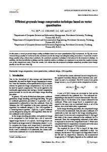
II. BACKGROUND Library cells are pre-characterized in the following way. Circuit-level simulations are performed on the CMOS gates, excited with voltage ramps with a range of slew values and loaded by a range of pure capacitance values. CSM library standards differ by the forms in which they store the simulation results. ECSM based characterization uses tables of cell voltage response tables. The characterization data is stored as tables of time-voltage waveforms (represented by time delays at which cell outputs cross a set of pre-defined voltage thresholds) for each combination of input slew and load capacitance, as shown in Figure 1. (a). CCS uses a similar characterization style; the main difference is that the characterization data is stored as tables of current (rather than voltage) as a function of time, as depicted in Figure 1. (b). The two raw characterization data sets are essentially equivalent and can be mapped from one to another. InSlew
CLoad (a)
III.
CSM WAVEFORM COMPRESSION
In this section we present two methods for library compression, constant-ratio compression and adaptive. The constant-ratio method uses projection in the same subspace for all waveforms, whereas the adaptive method tries to maintain the same error threshold for all compressed waveforms by using a different projection for each waveform. The efficiency of the PCA-based compression is greatly improved by a pre-processing procedure, described in the sequel, which focuses the algorithm toward retaining the features essential to timing analysis. We also highlight a timing interpretation associated with the first few principal components.
A. Waveform Preprocessing One of the key novelties of the proposed compression methods is a well crafted and effective preprocessing step during which all waveforms that are used for basis extraction will be "normalized" by a procedure described below. Orthogonal basis extraction will be subsequently performed on the normalized waveforms. We start with a database of time vectors representing the monotonic CSM time-vs-voltage waveforms for various cells in the library T = [t1 , t2 ,..., td ]
InSlew
CLoad (b) Figure 1. (a) ECSM Voltage Waveform Table, (b) CCS Current Waveform Table.
The storage of entire waveforms in the CSM methodology as opposed to just selected features (e.g., delay and slew) in traditional techniques represents an order-of-magnitude increase of the characterization data volume and calls for data compression, even at the cost of some accuracy. We adopt a common, and well-
(1)
Here tk, k = 1,…,d, represent the time instances at which the output waveform crosses a given voltage threshold Vk. The voltages are all assumed to be normalized to the 0-1V interval and the thresholds are expressed as percentages. First all waveforms are subjected to an affine transformation (shift and scale) which aligns all crossings of the, e.g., 10% threshold at time 0 and the, e.g., 90% crossing at time 1. Note that the threshold values are technology, library, and design methodology dependent and specified by the cell designers during characterization. The proposed scaling scheme has two advantages. First, since all the time values corresponding to the 10% and 90% thresholds are mapped onto the same set of values, the rank of database decreases by 2, which reduces the dimensionality and complexity of the original database, thereby, increasing its compressibility. Second, the 10% and 90% points are reconstructed more accurately, which is desirable for timing analysis. The next pre-processing step is averaging. In our application, each CSM waveform time vector is a data vector and time points t1
to td are variables. The chosen averaging operation centers entries of the database in the direction of each time vector (data-wise) not in the direction of variables (variable-wise). This kind of averaging has the advantage of introducing a new (low cost) basis vector (called the 0th basis and graphically shown in Figure 2. ), which is orthogonal to other basis vectors extracted by PCA. For most timing algorithms, only the difference between adjacent time points is required, therefore, the coefficient associated with this basis vector may not even need to be stored.
We assume that the original database is organized as a matrix, A, each row representing a preprocessed waveform as represented by Eq. (2). For a typical library there will be hundreds of thousands of rows. Principal component analysis [8] computes a new basis for representing the waveforms through the SVD algorithm. The SVD algorithm applied to matrix A yields the decomposition A = U ΣV ′
0
1
(2)
where Σ is a diagonal matrix of singular values in decreasing order and the rows of V represent an orthogonal basis of waveforms: the principal components. By setting the “small” singular values to zero, we obtain a low rank approximation of the original matrix, i.e., a representation in terms of a subset of basis vectors which is optimal in the sense of minimizing the “average” error.
time
Figure 2. The 0th basis vector.
Moreover, by centering time vectors around zero, the scaling and the subsequent weighting can be done symmetrically on the extremes of waveforms. Finally, the pre-processing procedure addresses the fact that not all portions of the waveform are equally relevant for the analysis. For example, given the properties of CMOS circuits, the exact behavior of the waveform under the 10% and over the 90% thresholds are less important for timing analysis. Therefore, ideally, the error introduced by compression should be distributed according to the accuracy needs of the timing algorithm. In our procedure we address this problem by differently weighting the various points in the original database, prior to the PCA step. We use small weights for the extreme points of waveforms in which we are less interested and larger weights for the intermediate points which are more significant for timing analysis. Using this simple procedure, we forgo some measure of optimality. Ideally weighting and the PCA analysis should be performed in tandem [9]. Nevertheless, simulation results indicate that our method is sufficiently accurate for waveform compression. Figure 3. summarizes the entire preprocessing procedure described in this section.
Scale
B. Constant ratio compression This subsection explains the constant-ratio compression method. In this method the number of coefficients for every compressed waveform is the same. The benefit of this method is its simplicity. However, this method needs to be accompanied with a causality enforcing procedure. By causality we mean the requirement that the crossing times tk, k = 1,…,d are monotonically increasing, an obvious property for time-voltage waveforms, which is not necessarily preserved by the approximation. In order to model each time vector with m principal coefficients, the constant-ratio compression algorithm works as follows: 1.
Time vector database extraction from the library,
2.
Preprocessing including shifting, scaling, averaging and weighting,
3.
Basis set extraction by using PCA as shown above,
4.
Coefficient calculation for m first basis vectors corresponding to the largest singular values,
5.
Causality enforcement for each compressed waveform.
The non-causality problem is a significant issue when the libraries with more complex gates are compressed. We propose the following procedure in conjunction with the constant ratio compression method to cope with the non-causality. a.
Check non-causality for every reconstructed time m
(a)
(b)
∑a P j
j
, where aj and Pj denote principal
j =0
Weighting
Averaging
(c)
vectors Tr =
(d)
Figure 3. Preprocessing steps (a) 1,715 waveforms from library, (b) scaling of aligned waveforms on 10% and 90%, (c) waveforms after averaging (d) waveforms after weighting.
coefficients and components, respectively. b. If Tr is non-causal then Solve min||T-Tr|| which means calculating aj, for j=0,…,m s.t. (ti)r < (ti+1)r for i = 1,…,m It is clear that the calculated aj from above procedure is not optimal in terms of the L2 norm criteria. Therefore above procedure might result in inaccurate compression. The proposed adaptive compression algorithm in next subsection results in high compression ratio for the same accuracy level while maintaining the causality condition.
First(red) and Second (blue) Components
1st, 2nd and 3rd coeeficients vs capacitances
Third(green) and Fourth (magenta) Components
1st, 2nd and 3rd coeeficients vs capacitances
1
1
0.6 Volt
0.4
0.4
0.2
0.2 0
-0.4
-0.2
0
0.2
0.4
0.6
0
-0.4
Scaled time
-0.2
0
0.2
0.4
0.6
Scaled time
(a)
(b)
Figure 4. Basis vectors (a) first and second basis vectors (red and blue respectively), (b) third and fourth basis vectors (green and magenta).
Figure 4. shows examples of basis waveforms for real libraries. It explains why arbitrary linear combinations of these waveforms do not guarantee causality in general. Nevertheless the dominant basis vectors reflect the true physical properties of the waveforms.
C. Adaptive Compression This section introduces an adaptive compression technique which achieves superior compression ratios and simultaneously solves the causality enforcement problem. This method adaptively chooses a number of coefficients for each waveform while meeting a specific required accuracy. The adaptive compression method is capable of checking non-causality during the coefficient selection and guarantees a causal reconstructed waveform. In order to compress each waveform with a maximum error ε0, the adaptive compression algorithm is composed of the following steps: 1.
Time vector extraction from the library,
2.
Preprocessing including shifting, averaging, scaling and weighting,
3. 4.
Basis set extraction by using PCA, Coefficient calculation for each waveform until the reconstructed waveform is causal and its error is less than the pre-specified error ε0.
IV. PARAMETERIZATION This section presents an additional parametric compression method which uses the principal coefficients obtained by the procedure in the previous section. Parametric compression, besides increasing the compression ratio, also provides waveform interpolation, i.e., it calculates the waveforms corresponding to input slews and load capacitances between the points provided in the model table [7].
0 Principal coefficients
0.8
0.6 Volt
0.8
Principal coefficients
0
-0.5
-1 -1.5
-2 0
0.01
0.02
0.03
0.04
0.05
-0.5 -1 -1.5 -2 0
0.06
0.005
0.01
Load capacitance
0.015
0.02
0.025
Load capacitance
Figure 5. First, second and third coefficients (red, blue and green respectively) versus load capacitance for two different gates.
Simulation shows that principal coefficients have a near-linear dependence on load capacitances (Figure 5. shows the first to third coefficients versus load capacitance for two example gates). Based on this observation, we propose a linear model for principal coefficients ai = fi(C) = k1+k2C. We also report the simulation results for a second order polynomial model ai = fi(C) = k1+k2C + k3C2. As mentioned before, parameterization allows higher compression and enables interpolation. A more general parametric compression is to express principal coefficients in terms of input slew and load capacitance and even PVT variables. Figure 6. shows the first component versus input slew and load capacitance for a typical gate. Here we present a bilinear and second order polynomial to present principal coefficients in terms of load capacitance and input slew. It becomes possible to extend the parametric representation to the complete PVT space, but this is outside the scope of the paper. Equations (3) and (4) describe bilinear and second order parameterization: ai = f i (C , S ) = k1 + k2C + k3 S + k 4C.S 2
2
ai = fi (C , S ) = k0 + ∑∑ kijC i S j
(3) (4)
i =1 j =1
Simulation results show that a bilinear representation has an acceptable accuracy for the ECSM timing analysis. Alternatively, coefficients can also be modeled by a two dimensional piecewise linear surface in the slew-capacitance (S-C) plane as shown by our studies of the the accuracy versus compaction tradeoff in the following results section.
Parametric compression represents the coefficients calculated by PCA as approximate analytical functions of input slews (S), load capacitances (C), and Process, Supply Voltage, Temperature, (PVT) variables, ai = fi(C, S,VPVT), where VPVT is the vector of all PVT variables. This form is significantly more compact than the tabular storage of PCA coefficients. Parametrization is useful even in the one dimensional case. For example, ECSM analysis uses waveforms (time and voltage) corresponding to a continuous range of load capacitances [7].
Figure 6. First coefficient in the slew-capacitance plane.
V. EXPERIMENTAL RESULTS This section presents simulation results for non-parametric and parametric compression techniques applied to the ECSM and CCS
libraries. Time, voltage and current units are nanosecond, volt and micro Amperes, respectively.
A. Constant-Ratio Compression To verify the accuracy and efficiency of the proposed techniques, the experiments are, first, carried out on a sample 65nm ECSM library with 35 CMOS gates, characterized at nominal process corner, 0.925 volt, and 125oC. Each gate is characterized for 7x7 (input slew, output capacitive load) combinations and for each of these combinations, a voltage waveform with 21 uniform voltage point increment ({0%, 0.05%, 0.10%,…, 0.95%, 100%} of VDD) is stored in the ECSM library which are shown in Figure 3. (a). The previously described pre-processing steps (shifting, scaling, averaging, weighting), described in Section III and shown in Figure 3. (b)-3(d), are performed on the the ECSM library. Note that the shifted and scaled waveforms cross at the 10% and 90% VDD transition times to maintain the accuracy level at 10% and 90% transition times of compressed waveforms. Figure 3. (c) presents the waveforms centered on the origin by using the averaging operation. Next, the first two and last two points of the voltage waveforms are weighted by 0.05 and 0.1, respectively, as illustrated in Figure 3. (d). TABLE I. summarizes the results for compression ratios as well as the compression error using different error probing criteria. Figure 7. (a) shows the absolute error of compressed waveforms (on the waveform of Figure 3. (d)) using the first four coefficients (82% library compression). The maximum L2-norm absolute error is 0.3 ps for the waveform shown in Figure 7. (b). The histogram in Figure 7. (a) also shows that, in most cases, using the first four coefficients, the L2-Norm absolute error diminishes exponentially, which confirms that adaptive compression technique is a better solution to achieve higher compression ratios. Waveform with maximum error
1 original reconstructed
0.6 0.4
0.3ps
0.2 0 0.4
0.5
0.6
0.7
0.8
0.9
Time
(a)
The next experiment, test the viability of using the basis set extracted from one process-voltage-temperature (PVT) corner to model (compress) the CSM library waveforms for another PVT corner. For this experiment, 8 2891-waveform libraries at 8 different PVT points are employed and the basis set extracted from one corner library is utilized to model the waveforms of the other seven CSM libraries). The maximum error was 1ps. TABLE I.
ERROR MEASUREMENT CRITERIA FOR 82% LIBRARY COMPRESSION
Exp
1
2 3 4
Max Error
Description
Weighted points
extremes
Un-weighted Weighted 50% point Weighted extreme points and rising/ falling classification
Type of Error Measurement
0.3ps
Absolute L2 norm
1.4%
Relative L2 norm
2%
Relative on 10%-90%
1.6%
Relative on 50% delay
0.64ps 0.5%
Absolute L2 norm Relative on 50% delay
0.12 %
Relative L2 norm
B. Adaptive Compression In this subsection we apply the adaptive compression algorithm to a 65nm ECSM library with 754 gates and 210,798 waveforms. This library includes wide range of gates including flip-flop, XOR, XNOR, Multiplexer, etc. Figure 8. (a) shows the compression ratio when the error adaptively changes from 1.5% to 0.01%. Figure 8. (b) shows the number of coefficients for each waveform. It has been observed that most voltage waveforms can be modeled with one to three coefficients while other voltage waveforms requires a larger set of coefficients to be modeled accurately (14 out of 21). The latter waveforms belong to gates with transmission gates such as XOR, XNOR, and Multiplexer. Adaptive compression results in 88% compression with maximum relative L2-norm error of 1.5%.
(b)
Figure 7. (a) Histogram of absolute error for 1,715 voltage waveforms, (b) the waveform with maximum error.
Number of coefficients for adaptive compression
14
Compression ratio
Other error measurement criteria have also been used to evaluate the quality of the proposed techniques as shown in TABLE I. . Experiment 1 of TABLE I. presents the maximum relative/absolute L2-norm error between the original ECSM voltage waveforms and the weighted compressed ones. As seen in this table, the compression with four coefficients yields sufficient accuracy levels with different error criteria. On the other hand, the experimental results show that if the compression is done without weighting preprocessing step, the compression error for the points between 10% to 90% transition times can be doubled (experiment 2 in TABLE I. ). For experiment 3 in TABLE I. , 50% transition time is emphasized during compression. This experiment shows a 3-fold reduction in compression error compared to un-weighted compression strategy. Experiment 4 in TABLE I. confirms that raising and falling transitions can be efficiently compressed using
Compression vs error for ECM library
90
85
Number of coefficients
Vltage
0.8
a common basis. The maximum errors for compressing separately falling and rising waveforms are 0.12ps and 0.2ps, respectively, only slightly better than the maximum error of 0.3ps for uncategorized voltage waveforms.
80
75
12 10 8 6 4 2
70 0
0.005
0.01
Relative error
(a)
0.015
0
0.5
1
1.5
W aveform number
2 x 10
5
(b)
Figure 8. (a) Error versus compression for adaptive method, (b) number of coefficients for 88% compression.
C. CCS Library Compression In this subsection, the simulation results for CCS waveform compression are reported. The Nangate CCS public library which has 71,616 current waveforms has been used for this experiment.
Figure 9. (a) demonstrates a few CCS current waveforms. The preprocessing consists of scaling in time and current. Figure 9. (b) shows adaptive compression ratio versus relative error. For a relative error of 10%, the adaptive compression ratio is 76%. The reconstructed waveform with maximum error is shown in Figure 9. (c), which demonstrates the accuracy of waveform reconstruction.
2) Multi Variable We divide the C-S plane to shown in Figure 6. to 4×4 equal regions and then model the principal coefficients of each gate by using a linear surface (piecewise linear). As shown in Figure 11. (a), the maximum L2-norm error is 0.6ps with 93% compression. A bilinear model for principal coefficients of voltage waveform (c.f. Figure 11. (b)) yields a larger compression ratio of 98% with the maximum error of 1.4ps.
Current waveform
140 120
Current
100 80 1.4ps
0.6ps
60 40 20 0 0
0.2
0.4
0.6
0.8
1
(a)
Scaled time
(a) 3
Compression vs error for CCS library
80
original reconstructed
60
2
Current
Compression ratio
2.5
40
VI.
0
0.5
0.02
0.04
0.06
Relative error
(b)
0.08
0.1
CONCLUSION
1.5 1
20
(b)
Figure 11. Error histogram for (a) piecewise linear, (b) bilinear coefficient modeling.
Current waveform with maximum error
0 0
0.2
0.4
0.6
0.8
1
Time
(c)
Figure 9. (a) Typical current waveforms, (b) relative error vs compression, (c) waveform with maximum relative error 10%.
D. Parameterization This subsection shows the parametric compression for slew and capacitance. The 65nm ECSM library with 1,715 voltage waveforms is utilized for simulation. 1) One Variable We use the first order polynomial to model fi mentioned in section IV as a one-dimensional linear function of load capacitance. Figure 10. shows the absolute error histogram and the worst reconstructed waveform with maximum L2-norm error of 1.2ps (the error without parameterization is 0.3ps). Note that using one-dimensional second order polynomial function yields maximum L2-norm error of 1.15ps.
A linear-algebra-based compression technique, PCA, was utilized to reduce the size of the CSM libraries. The technique was applied to several 65nm, ECSM and CCS libraries. The simulation results proved the high accuracy and large compression ratio of the proposed technique. Moreover this paper presented a parametriccompression which results in further compression and an analytical interpolation model for waveform computation. In future we plan to augment the PCA-based parameterized model considering voltage, temperature, and process-related sources of variations.
REFERENCES [1] R. Trihy, “Addressing library creation challenges from recent liberty extensions”, Proc. of Design Automation Conference, pp 474-479, 2008.
[2] http://www.cadence.com/Alliances/languages/Pages/ecsm.aspxRef3 [3] http://www.synopsys.com/products/solutions/galaxy/ccs/ccs_faq.html [4] http://www.nangate.com/index.php?option=com_content&task=view&i d=83&Itemid=102
[5] V. Zolotov and J. Xiong and S. Abbaspour, D.J. Hathaway and C. Visweswariah, “Compact modeling of variational waveforms,” Proc. of International Conference on Computer Aided Design, pp 705-712, 2007.
[6] A. Ramalingam, A.K. Singh, S.R. Nassif, M. Orshansky, “Accurate Waveform Modeling using Singular Value Decomposition with Applications to Timing Analysis,” Proc. of Design Automation Conference, pp 148-153, 2007.
[7] P. Feldmann, S. Abbaspour, D. Sinha, G. Schaeffer, R. Banerji, H. 1.2ps
Gupta, “Driver Waveform Computation for Timing Analysis with Multiple Voltage Threshold Driver Models,” Proc. of Design Automation Conference, pp 425-428, 2008.
[8] I.T. Jolliffe, Principal component analysis, 2nd edition. Springer, New York, 2002. Figure 10. Error histogram for waveform compression for one dimensional linear parameterization.
[9] N. Srebro, T. Jaakkola, “Weighted Low-Rank Approximations,” Proc. of International Conference Washington DC, 2003.
on
Machine
Learning
(ICML-2003),