against deterministic timed automata (DTA) objectives practical. We show .... works [4,9] provide a quantitative interpretation to timed automata where delays of.
Efficient CTMC Model Checking of Linear Real-Time Objectives Benoˆıt Barbot2 , Taolue Chen3 , Tingting Han1 , Joost-Pieter Katoen1,3 , and Alexandru Mereacre1 1
MOVES, RWTH Aachen University, Germany 2 ENS Cachan, France 3 FMT, University of Twente, The Netherlands
Abstract. This paper makes verifying continuous-time Markov chains (CTMCs) against deterministic timed automata (DTA) objectives practical. We show that verifying 1-clock DTA can be done by analyzing subgraphs of the product of CTMC C and the region graph of DTA A. This improves upon earlier results and allows to only use standard analysis algorithms. Our graph decomposition approach naturally enables bisimulation minimization as well as parallelization. Experiments with various examples confirm that these optimizations lead to significant speed-ups. We also report on experiments with multiple-clock DTA objectives. The objectives and the size of the problem instances that can be checked with our prototypical tool go (far) beyond what could be checked so far.
1 Introduction For more than a decade, the verification of continuous-time Markov chains, CTMCs for short, has received considerable attention, cf. the recent survey [7]. Due to unremitting improvements on algorithms, (symbolic) data structures and abstraction techniques, CTMC model checking has emerged into a valuable analysis technique which – supported by powerful software tools– has been adopted by various researchers for systems biology, queueing networks, and dependability. The focus of CTMC model checking has primarily been on checking stochastic versions of the branching temporal logic CTL, such as CSL [6]. The verification of LTL objectives reduces to applying well-known algorithms [20] to embedded discrete-time Markov chains (DTMCs). Linear objectives equipped with timing constraints, have just recently been considered. This paper treats linear real-time specifications that are given as deterministic timed automata (DTA). These include, e.g., properties of the form: what is the probability to reach a given target state within the deadline, while avoiding “forbidden” states and not staying too long in any of the “dangerous” states on the way. Such properties can neither be expressed in CSL nor in dialects thereof [5,14]. Model checking DTA objectives amounts to determining the probability of the set of paths of CTMC C that are accepted by the DTA A, i.e., Prob (C |= A). We recently showed in [12] that this equals the reachability probability in a finite piecewise deterministic Markov process (PDP) that is obtained by a region construction on the product C ⊗ A. This paper reports on how to make this approach practical, i.e., how to efficiently realize CTMC model checking against DTA objectives. P.A. Abdulla and K.R.M. Leino (Eds.): TACAS 2011, LNCS 6605, pp. 128–142, 2011. c Springer-Verlag Berlin Heidelberg 2011 �
Efficient CTMC Model Checking of Linear Real-Time Objectives
129
As a first step, we show that rather than taking the region graph of the product C ⊗ A, which is a somewhat ad-hoc mixture of CTMCs and DTA, we can apply a standard region construction on DTA A prior to building the product. This enables applying a standard region construction for timed automata. The product of this region graph with CTMC C yields the PDP to be analyzed. Subsequently, we exploit that for 1clock DTA, the resulting PDP can be decomposed into subgraphs—each of which is a CTMC [12]. In this case, Prob (C |= A) is the solution of a system of linear equations whose coefficients are transient probability distributions of the (slightly amended) subgraph CTMCs. We adapt the algorithm for lumping [13,19] on CTMCs to our setting and prove that this preserves reachability probabilities, i.e., keeps Prob (C |= A) invariant. As the graph decomposition naturally enables parallelization, our tool implementation also supports the distribution of computing transient probabilities over multiple multi-core computers. Finally, multi-clock DTA objectives –for which the graph decomposition does not apply– are supported by a discretization of the product PDP. Three case studies from different application fields are used to show the feasibility of this approach. The first case study has been taken from [3] which considers 1-clock DTA as time constraints of until modalities. Although using a quite different approach, our verification results coincide with [3]. The running time of our implementation (without lumping and parallelization) is about three orders of magnitude faster than [3]. Other considered case studies are a randomly moving robot, and a real case study from systems biology [15]. Bisimulation quotienting (i.e., lumping) yields state space reduction of up to one order of magnitude, whereas parallelizing transient analysis yields speedups of up to a factor 13 on 20 cores, depending on the number of subgraphs in the decomposition. The discretization approach for multi-clock DTA may give rise to large models: checking the robot example (up to 5,000 states) against a two-clock DTA yields a 40million state DTMC for which simple reachability probabilities are to be determined. Related work. The logic asCSL [5] extends CSL by (time-bounded) regular expressions over actions and state formulas as path formulas. CSLTA [14] allows 1-clock DTA as time constraints of until modalities; this subsumes acCSL. The joint behavior of C and DTA A is interpreted as a Markov renewal process. A prototypical implementation of this approach has recently been reported in [3]. Our algorithmic approach for 1-clock DTA is different, yields the same results, and is –as shown in this paper– significantly faster. Moreover, lumping is not easily possible (if at all) in [3]. In addition, it naturally supports bisimulation minimization and parallelization. Bisimulation quotienting in CSL model checking has been addressed in [18]. The works [4,9] provide a quantitative interpretation to timed automata where delays of unbounded clocks are governed by exponential distributions. Brazdil et al. present an algorithmic approaches towards checking continuous-time stochastic games (supporting more general distributions) against DTA specifications [11]. To our knowledge, tool implementations of [4,9,11] do not exist. Organization of the paper. Section 2 provides the preliminaries and summarizes the main results of [12]. Section 3 describes our bisimulation quotienting algorithm. Section 4 reports on the experiments for 1-clock DTA objectives. Section 5 describes the
130
B. Barbot et al.
discretization approach and gives experimental results for multi-clock DTA. Finally, Section 6 concludes. (Proofs are omitted and can be found in the full version available at http://moves.rwth-aachen.de/i2/han.)
2 Preliminaries 2.1 Continuous-Time Markov Chains Definition 1 (CTMC). A (labeled) continuous-time Markov chain (CTMC) is a tuple C = (S, AP, L, α, P, E) where S is a finite set of states; AP is a finite set of atomic propositions; L : S → 2AP is the labeling function; α ∈ Distr(S) is the initial distribution; P : S × S → [0, 1] is a stochastic matrix; and E : S → R�0 is the exit rate function. Here, Distr (S) is the set of probability distributions on set S. The probability to exit �t state s in t time units is given by 0 E(s)·e−E(s)τ dτ . The probability to take the transi�t tion s → s� in t time units is P(s, s� )· 0 E(s)e−E(s)·τ dτ . The embedded DTMC of C t0 t1 is (S, AP, L, α, P). A (timed) path in CTMC C is a sequence ρ = s0 −− → s1 −− → s2 · · · C such that si ∈ S and ti ∈ R>0 . Let Paths be the set of paths in C and ρ[n] := sn be the n-th state of ρ. The definitions of a Borel space on paths through CTMCs,and the probability measure Pr follow [20,6]. r2 {a}
1
s0 r0
{a}
0.2
a, x < 1, ∅
{b} s2
1
0.5
r1
b, x > 1, ∅
q0
s1 s3
0.3 r3
q1
1 {c}
(a) An example CTMC
a, 1 < x < 2, {x}
(b) An example DTA
Fig. 1. Example CTMC and DTA
Example 1. Fig. 1(a) shows an example CTMC with AP = {a, b, c} and initial state s0 , i.e., α(s) = 1 iff s = s0 . The exit rates are indicated at the states, whereas the transition 2.5 1.4 2 −→ s1 −− −→ s0 −→ probabilities are attached to the edges. An example path is ρ = s0 −− 2π s1 −−→ s2 · · · with ρ[2] = s0 and ρ[3] = s1 . Definition 2 (Bisimulation). Let C = (S, AP, L, α, P, E) be a CTMC. Equivalence relation R on S is a (strong) bisimulation on C if for s1 Rs2 : L(s1 ) = L(s2 ) and P(s1 , C) = P(s2 , C) for all C in S/R and E(s1 ) = E(s2 ). Let s1 ∼ s2 if there exists a strong bisimulation R on C with s1 Rs2 . The quotient CTMC under the coarsest bisimulation ∼ can be obtained by partitionrefinement with time complexity O(m log n) [13]. A simplified version with the same complexity is recently proposed in [19].
Efficient CTMC Model Checking of Linear Real-Time Objectives
131
2.2 Deterministic Timed Automata Clock variables and valuations. Let X = {x1 , . . ., xn } be a set of clocks in R�0 . An X -valuation (valuation for short) is a function η : X → R�0 ; 0 is the valuation that assigns 0 to all clocks. A clock constraint g on X has the form x �� c, or g � ∧ g �� , where x ∈ X , �� ∈ {, �} and c ∈ N. Diagonal clock constraints like x−y �� c do not extend the expressiveness [8], and are not considered. Let CC(X ) denote the set of clock constraints over X . An X -valuation η satisfies constraint g, denoted as η |= g if η(x) �� c for g of the form x �� c, or η |= g � ∧ η |= g �� for g of the form g � ∧ g �� . The reset of η w.r.t. X ⊆ X , denoted η[X := 0], is the valuation η � with ∀x ∈ X. η � (x) := 0 and ∀x ∈ / X. η � (x) := η(x). For δ ∈ R�0 , η+δ is the valuation η �� such that ∀x ∈ X . �� (x) := η(x) + δ. η Definition 3 (DTA). A deterministic timed automaton (DTA) is a tuple A = (Σ, X , Q, q0 , QF , →) where Σ is a finite alphabet; X is a finite set of clocks; Q is a nonempty finite set of locations; q0 ∈ Q is the initial location; QF ⊆ Q is a set a,g,X of accepting locations; and → ∈ (Q \ QF )×Σ×CC(X )×2X ×Q satisfies: q −− −−→ q � �
�
a,g,X and q −− −−−→ q �� with g = g � implies g ∩ g � = ∅. a,g,X We refer to q −− −−→ q � as an edge, where a ∈ Σ is the input symbol, the guard g is a clock constraint on the clocks of A, X ⊆ X is a set of clocks and q, q � are locations. The intuition is that the DTA A can move from location q to q � on reading the input symbol a if the guard g holds, while resetting the clocks in X on entering q � . By convention, we assume q ∈ QF to be a sink, cf. Fig. 1(b). a0 ,t0 an ,tn −−→ q1 · · · qn −− −−→ qn+1 Paths. A finite (timed) path in A is of the form θ = q0 −− with qi ∈ Q, ti > 0 and ai ∈ Σ (0 � i � n). The path θ is accepted by A if θ[i] ∈ QF for some 0 � i � |θ| and for all 0 � j < i, it holds that η0 = 0, ηj +tj |= gj and ηj+1 = (ηj +tj )[Xj := 0], where ηj is the clock valuation on entering t0 t1 qj and gj the guard of qi − → qi+1 . The infinite path ρ = s0 −− → s1 −− → · · · in CTMC tn−1 t0 C is accepted by A if for some n ∈ N, s0 −−→ s1 · · · sn−1 −−−−→ sn induces the DTA L(sn−1 ),tn−1 L(s ),t0 path ρˆ = q0 −−−−0−−→ q1 · · · qn−1 −−−− −−−−−→ qn , which is accepted by A. The set of CTMC paths accepted by a DTA is measurable [12]; our measure of interest is given by: Prob(C |= A) = Pr{ ρ ∈ Paths C | ρˆ is accepted by DTA A }.
Regions. Regions are sets of valuations, often represented as constraints. Let Re(X ) be the set of regions over X . For regions Θ, Θ� ∈ Re(X ), Θ� is the successor region of Θ if for all η |= Θ there exists δ ∈ R>0 such that η + δ |= Θ� and ∀δ � < δ. η + δ � |= Θ ∨ Θ� . The region Θ satisfies a guard g, denoted Θ |= � g, iff ∀η |= Θ. η |= � g. The reset operation on region Θ is defined as Θ[X := 0] := η[X := 0] | η |= Θ . Definition 4 (Region graph [2]). Let A = (Σ, X , Q, q0 , QF , →) be a DTA. The region graph G(A) of A is (Σ, W, w0 , WF , ���) with W = Q × Re(X ) the set of states; w0 = (q0 , 0) the initial state; WF = QF × Re(X ) the set of final states; and ��� ⊂ W × ((Σ × 2X ) { δ }) × W the smallest relation such that:
132
B. Barbot et al. δ
(q, Θ) ��� (q, Θ� ) if Θ� is the successor region of Θ; and a,X
a,g,X (q, Θ) ��� (q � , Θ� ) if ∃g ∈ CC(X ) s.t. q −− −−→q � with Θ |= g and Θ[X := 0] = Θ� .
Product. Our aim is to determine Prob(C |= A). This can be accomplished by computing reachability probabilities in the region graph of C ⊗ A where ⊗ denotes a product construction between CTMC C and DTA A [12]. To ease the implementation, we consider the product C ⊗ G(A). Definition 5 (Product). The product of CTMC C = (S, AP, L, α, P, E) and DTA region graph G(A) = (Σ, W, w0 , WF , ���), denoted C ⊗G(A), is the tuple (V, α� , VF , Λ,
→) with V = S × W , α� (s, w0 ) = α(s), VF = S × WF , and �� � � – → ⊆ V × [0, 1] × 2X {δ} × V is the smallest relation such that: δ
δ
• (s, w) → (s, w� ) iff w ��� w� ; and p,X
L(s),X
• (s, w) → (s� , w� ) iff p = P(s, s� ), p > 0, and w ��� w� . – Λ : V → R�0 is the exit rate function where: � p,X E(s) if (s, w) → (s� , w� ) for some (s� , w� ) ∈ V Λ(s, w) = 0 otherwise. The (reachable fragment of the) product of CTMC C in Fig. 1(a) and the region graph of DTA A in Fig. 1(b) is given in Fig. 2. It turns out that C ⊗ G(A) is identical to G(C ⊗ A), the region graph of C ⊗ A as defined in [12]. Theorem 1. For any CTMC C and any DTA A, C ⊗ G(A) = G(C ⊗ A). As a corollary [12], it follows that Prob(C |= A) equals the reachability probability of the accepting states in C ⊗ G(A). In addition, C ⊗ G(A) is a PDP. 2.3 Decomposition for 1-Clock DTA Let A be a 1-clock DTA and {c0 , . . . , cm } ⊆ N with 0 = c0 < c1 < · · · < cm the constants appearing in its clock constraints. Let Δci = ci+1 −ci for 0 � v , r v1 , r0 0 0 i < m. The product C ⊗ G(A) can δ s0 , q0 , 0�x