Efficient Deep Neural Network for Digital Image Compression

Hindawi Publishing Corporation Journal of Sensors Volume 2016, Article ID 3184840, 7 pages http://dx.doi.org/10.1155/2016/3184840

Research Article Efficient Deep Neural Network for Digital Image Compression Employing Rectified Linear Neurons Farhan Hussain and Jechang Jeong Department of Electronics & Computer Engineering, Hanyang University, Seoul 133-791, Republic of Korea Correspondence should be addressed to Jechang Jeong; [email protected] Received 16 December 2014; Accepted 11 February 2015 Academic Editor: Wei Wu Copyright © 2016 F. Hussain and J. Jeong. This is an open access article distributed under the Creative Commons Attribution License, which permits unrestricted use, distribution, and reproduction in any medium, provided the original work is properly cited. A compression technique for still digital images is proposed with deep neural networks (DNNs) employing rectified linear units (ReLUs). We tend to exploit the DNNs capabilities to find a reasonable estimate of the underlying compression/decompression relationships. We aim for a DNN for image compression purpose that has better generalization property and reduced training time and support real time operation. The use of ReLUs which map more plausibly to biological neurons, makes the training of our DNN significantly faster, shortens the encoding/decoding time, and improves its generalization ability. The introduction of the ReLUs establishes an efficient gradient propagation, induces sparsity in the proposed network, and is efficient in terms of computations making these networks suitable for real time compression systems. Experiments performed on standard real world images show that using ReLUs instead of logistic sigmoid units speeds up the training of the DNN by converging markedly faster. The evaluation of objective and subjective quality of reconstructed images also proves that our DNN achieves better generalization as most of the images are never seen by the network before.

1. Introduction Digital image compression plays an extremely important role in the transmission and storage of digital image data. Usually the amount of data associated with visual information is so large that its storage requires enormous memory and its transmission requires high bandwidths. Image compression is the process of effectively coding digital images to reduce the number of bits required to represent an image. This compression allows transmission of image at very low bandwidths and minimizes the space requirement for storage of this data. As consecutive frames of still images constitute the video data, algorithms designed for 2D still image compression can be effectively extended to compress video data. The image compression algorithms can be broadly classified into lossless and lossy compression algorithms. A lossless compression algorithm reproduces the original image exactly without any loss of information. These methods are used in applications where data loss is unacceptable, for example, text data and medical images. In this paper we are going to target the lossy

compression where the reproduced image is not an exact replica of the original image. Some information is lost in the coding process. These algorithms provide a way of tradeoff between the image quality and the degree of compression. The goal is to achieve higher degree of compression without much degradation in image quality. Artificial neural networks (ANNs) [1–3] get their inspiration from the manner in which human brain performs calculations and makes decisions. In fact ANNs tend to imitate the functionality of human brain, that is, the biological neuron system. An ANN achieves this abstraction and modeling of the information processing capabilities of human brain by interconnecting a large number of simple processing elements called the artificial neurons. An artificial neuron is an electronically modeled biological neuron. The complexity of a real biological neuron is highly abstracted while modeling an artificial neuron. The theme is to mimic the working of human nervous system with the help of these artificial neurons. In order to achieve this each artificial neuron is

2 equipped with some computational strength similar to that possessed by a biological neuron. An artificial neuron like a biological neuron can take many input signals and then based on an internal weighting system produces a single output signal that is typically sent as input to another neuron. Figure 1 shows a representation of an artificial neuron. Here 𝑋0 , 𝑋1 , . . . , 𝑋𝑛 are the 𝑛 input signals to the artificial neuron. Each of these input signals is multiplied by a connection weight. These weights are represented by 𝑊0 , 𝑊1 , . . . , 𝑊𝑛 , respectively. All of these products are summed and fed to an activation function to generate an output for the artificial neuron. An ANN is set up by creating connections between these artificial neurons analogous to the connection between biological neurons in a human nervous system as shown in Figure 2. Recent developments in the processing capabilities of the CPU and advancement in the architecture of neural networks have attracted many researchers from various scientific disciplines to investigate these networks as a possible solution to solve various problems encountered in the fields of pattern recognition, prediction, optimization, function approximation, clustering, categorizing, and many more. ANNs are also being researched and developed to address the problem of compression of still images and video data [4–11] besides the conventional algorithms [12]. The target is to achieve high compression ratios, maximize the quality of reproduced images, and design systems that utilize minimum computational resources and support real time applications. In this work we attempt for these goals by a deep neural network [13], that is, an artificial neural network having multiple hidden layers of neurons between the input and output layers. These DNNs can model complex nonlinear relationships more efficiently. The extra layers of the DNNs enable the network to capture the highly variant features of the input and learn more higher abstract representations of the data. The common issues for the DNNs are that its training is time consuming and is computationally very expensive. In this work we propose a DNN for still image compression that has much reduced training time and is computationally efficient. Our DNN achieves this speed-up in training time and reduction in complexity by employing rectified linear units [14]. This arrangement also leads to better generalization of the network and reduces the real compression-decompression time. The network meets the targets guaranteed for a good compression system; it converges fast, does not have a vanishing gradient problem, and has a sparse representation (only part of the network is active for a given input). These characteristics make the proposed network suitable for real time compression systems. The rest of the paper is organized as follows. Section 2 gives a brief overview of the literature concerning image compression via ANNs and states the preliminaries. Section 3 introduces the proposed DNN. Section 4 reports the experimental results. Section 5 provides the conclusion to the paper.

2. Background and Preliminaries Several studies have been proposed to address the problem of digital image compression via artificial neural networks.

Journal of Sensors The most elemental and simple network, that is, the single structured neural network, is described in [4]. This network uses a 3-layer network with logistic transfer function to achieve image compression. Parallel architectures for neural networks for image compression are proposed in [5–7]. The idea is to compress different part of an image (i.e., according to some complexity) by different neural networks in parallel in order to increase the compression ratio and quality of reconstructed images. In [8] the authors propose the use of novel normalization function along with the single structured neural network to improve the compression quality. An ANN for calculating the discrete cosine transform for image compression is described in [9]. The authors in [10, 11] provide a summary of different neural network models and techniques such as vector quantization that neural networks can be complemented with to improve the compression results. The process of image compression can be formulated as designing a compressor and decompressor module as shown in Figure 3, where 𝐼 is the original image, 𝐼𝑐 is the compressed data, and 𝐼󸀠 is the reconstructed image. The number of bits in the compressed data is much less than the number of bits required to represent the original image. Usually these modules are realized by heavy complex algorithms with a lot of complicated calculations involved. As described before many researches are carried out to approximate the image compression/decompression modules with the help of ANN by generating an internal data representation. These networks are trained on several training images (inputoutput pairs), the task being to approximate the corresponding compression-decompression algorithm compactly and model it so it can be generalized to a large set of test data. This is achieved by rigorously training the network with the help of learning algorithms. This training process is characterized by the use of a given output that is compared to the predicted output and by adaption of all parameters according to this comparison. The parameters of a neural network are its weights. This paper uses the back propagation for training the ANN. The back propagation [15] is a supervised learning algorithm and is especially suitable for feedforward networks. The feed-forward neural networks refer to multilayer perceptron network in which the outputs from all the neurons go to following but not the preceding layers, so there are no feedback loops and the information flows in only one direction. The term back propagation is abbreviated for “backward prorogation of errors” and it implies that the errors (and therefore the learning) propagate backwards from the output nodes to the inner nodes. Hence back propagation is used to calculate the gradient of the error with respect to the network’s modifiable weights. This gradient is then used in a simple gradient descent algorithm to find weights that minimize the error. The term back propagation refers to the entire procedure encompassing both the calculation of gradient and its use in gradient descent. Back propagation requires that the transfer function used by the artificial neurons (or “nodes”) to be differentiable. Figure 2 shows a generalized architecture for an ANN. The neurons are tightly interconnected and organized into different layers. The input layer receives the input; the output layer produces the final

Journal of Sensors

3 W0

X0

W1

Input

X1 X2 . ..

Summer

Xn

W2

Bias

Wn

Activation function

Output

1

Figure 1: An artificial neuron.

ReLU

ReLU

ReLU

ReLU

ReLU

ReLU

ReLU

ReLU

ReLU

ReLU

ReLU

ReLU

ReLU

ReLU

ReLU

ReLU

ReLU

ReLU

ReLU

ReLU

ReLU

ReLU

ReLU

ReLU

ReLU

ReLU

ReLU

ReLU

ReLU

ReLU

ReLU

ReLU

Encoder

Decoder

Figure 2: Deep neural network architecture for image compression. Original image (I) of size M bits

Compression module

Compressed data (Ic ) of size N bits

Decompression module

Reconstructed image (I󳰀 )

Figure 3: Block diagram of an image compression system.

4

Journal of Sensors

output. Usually one or more hidden layers are sandwiched in between the two.

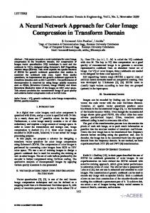
3. Proposed Deep Neural Network for Image Compression In this paper digital image compression is achieved by a deep neural network that employs rectified linear units. The multiple hidden layers of the DNN are advantageous in realizing more efficient internal data representations of the underlying compression-decompression function. Researchers conclude that the biological neurons can be better approximated and modeled by the ReLUs. As these ReLUs are more biologically plausible they can be engaged as better activation functions than the widely used logistic sigmoid and hyperbolic tangent functions. The ReLU is given by rectifier (𝑥) = max (0, 𝑥) ,

(1)

where 𝑥 is the input to the neuron. The function behaves linearly for a favorably excitatory input pattern and “0” otherwise. As can be seen the function is one sided; it does not possess the property of sign symmetry or antisymmetry. The function is not differentiable at “0” and its derivative, whenever it exists, can take only two values, “0” or “1.” Although the ReLUs are not entirely differentiable, nor symmetric and possess hard linearity they can outperform the sigmoid and hyperbolic tangent neurons. Experiments show that the ReLUs are worth the tradeoff with these much sophisticated counter parts. They allow fast convergence and better generalization of the DNN. These ReLUs are computationally much cheaper. The efficient computations required for both its value and its partial derivatives enable much larger network implementations. Engaging ReLUs induces sparsity in the network; that is, only a subset of neurons are active in the hidden layers. This leads to faster computation and better learning. Other advantages of sparsity are discussed in [14]. The DNN with ReLUs used for still image compression is shown in Figure 2. The network consists of an input layer, 𝑛 number of hidden layers, and an output layer. As this network is targeting image compression/decompression it must have equal number of input and output neurons, 𝑁 (an 𝑁 dimensional input is mapped to an 𝑁 dimensional output). The number of neurons in the input layer or the output layer corresponds to the size of image block to be compressed. Compression can be achieved by allowing the number of neurons at the last hidden layer, 𝐾, to be less than that of the neurons at both the input and the output layers (𝐾 < 𝑁). The number of hidden layers and hidden neurons is determined by the number of input and output neurons as well as desired compression ratio. The compression ratio of this DNN is the ratio of input neurons to the number of neurons in the last hidden layers. The training of the DNN is carried out with a set of images selected from the training set. The training images are divided into nonoverlapping blocks of size 𝑊 by 𝑊 pixels. The pixels in each of these blocks are normalized by a normalizing function 𝑓, usually from a grey scale value between 0 and 255 to a range of values between 0 and 1. These

normalized blocks are fed into the input layer of the DNN at random; each neuron in the input layer corresponds to one pixel; that is, 𝑁 = 𝑊 × 𝑊. As in case of supervised learning the desired output for the network is known in advance, which in case of image compression purpose is the same as the input to the network. We tend to resolve the network to produce at the output what it sees at the input. As we use back propagation for training the DNN, the difference between the actual output and desired output is calculated and the error is propelled backwards to adjust the parameters of the network accordingly. With the new weights the output is again calculated and compared with the desired one, errors are repropagated, the parameters are readjusted, and the process continues in an iterative fashion. In our implementation of DNN the training is stopped when the iterations reach their maximum limit or when the average mean square error drops below a certain threshold. Once the training of the network is completed, the parameters of the network are saved. With these finalized weights we utilize this DNN to compress and decompress the test images. The test image to be compressed is divided into nonoverlapping blocks. Each block is fed into the input of the network after normalization. The input layer and the 𝑛 hidden layers act as the compressor module and perform a nonlinear and nonorthogonal transformation 𝑆. The compressed data is found at the output of the last hidden layer. The output layer acts as the decompressor module and reconstructs the normalized input data block by performing a second transformation 𝑇. The decompressed image block can be found at the output neurons of the output layer. The dynamic range of the reconstructed data block is restored by applying the inverse normalization function 𝑓−1 . The transformations 𝑆 and 𝑇 are optimized by training the network on several training images.

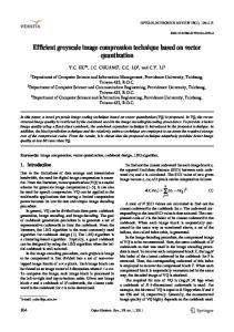
4. Experimental Results Experiments were performed on test images taken from the standard set of images: Lena, baboon, cameraman, pepper, and boats. The size of the test images was 512 by 512. The number of neurons in the input layer, output layer, and the last hidden layer was adjusted to achieve different compression ratios, that is, 4 : 1, 8 : 1, and 16 : 1. The epoch versus mean square error (mse) curves for the DNN employing the rectified linear neurons and the logistic sigmoid neurons were plotted for different compression ratios (CRs) and are shown in Figures 4–6. A comparison of these plots shows that the DNN with ReLUs converges several orders of magnitude faster than the one with logistic sigmoid units. This fact is illustrated in Figure 7 which shows that to reduce the mse to 0.0019 the DNN with sigmoid neurons takes 500 epochs while the same mse is achieved by the DNN with ReLUs after 50 epochs for a CR of 4 : 1. Similarly it takes 500 epochs for the sigmoid neurons to reduce the mse to 0.0039 at a CR of 8 : 1 while the same is achieved after 35 epochs by employing ReLUs. This high convergence rate validates the fact that the network with ReLUs trains much faster than their logistic counterparts.

5

0.04

0.09

0.035

0.08

0.03

0.07

0.025

0.06

0.02

0.05

mse

mse

Journal of Sensors

0.015

0.04

0.01

0.03

0.005

0.02

0

0.01 0

200

400

600

0

Epochs

0

200

400

600

Epochs

ReLU Sigmoid

Figure 4: Comparison of epoch versus mse for rectified linear neurons and logistic sigmoid neurons at a CR of 8 : 1.

ReLU Sigmoid


0.04 0.035

600

0.03

500

0.015

(16 : 1)

300 200

0.01

100

0.005 0

(8 : 1)

400

0.02

Epochs

mse

0.025

(4 : 1)

0 0

200

400

600

0.0019

Epochs


The performance of the network is measured by the peak signal to noise ratio (PSNR) of image reconstructed at the output layer and is defined as MAX𝐼 2 ), MSE

(2)

where MAX𝐼 is the maximum possible pixel value of the image and MSE is the mean square error given by MSE =

0.0075

Sigmoid ReLU

ReLU Sigmoid

PSNR = 10 log10 (

0.0039 mse

1 𝑚−1 𝑛−1 2 ∑ ∑ [𝐼 (𝑖, 𝑗) − 𝐼𝑅 (𝑖, 𝑗)] , 𝑚𝑛 𝑖=0 𝑗=0 𝑂

(3)

where 𝑚 and 𝑛 represent the size of the image in the horizontal and vertical dimensions, respectively, 𝐼𝑂 is the

Figure 7: Epochs required to reduce the mean square error of the DNN using sigmoid neurons and rectified linear neurons at different CRs.

original image, and 𝐼𝑅 is the reconstructed image. Tables 1–3 show the PSNR achieved by the set of five standard real world images compressed at different compression ratios by (i) the rectified linear DNN and (ii) the logistic sigmoid DNN. The DNNs were trained using the same data set and by the back propagation algorithm. There is a significant improvement in the PSNR of the reconstructed images for rectified linear units compared to the logistic units. This result proves better generalization ability of our network with ReLUs as none of the sequences in Tables 1–3 were used for the training of the DNN. To evaluate the subjective quality of the decompressed images Figures 8–10 show some of the original images and their reconstructed counterparts.

6

Journal of Sensors

(a)

(b)

(c)

Figure 8: (a) Original image, (b) image reconstructed by rectified deep neural network at a CR of 8 : 1, and (c) image reconstructed by deep neural network employing sigmoid transfer function at a CR of 8 : 1.

(a)

(b)

(c)

Figure 9: (a) Original Image, (b) image reconstructed by rectified deep neural network at a CR of 4 : 1, and (c) image reconstructed by deep neural network employing sigmoid transfer function at a CR of 4 : 1.

(a)

(b)

(c)

Figure 10: (a) Original image, (b) image reconstructed by rectified deep neural network at a CR of 16 : 1, and (c) image reconstructed by deep neural network employing sigmoid transfer function at a CR of 16 : 1.

Table 1: PSNR of the reconstructed images at a CR of 8 : 1.

Table 2: PSNR of the reconstructed images at a CR of 4 : 1.

Sequence

Compression scheme ReLU Sigmoid

Sequence


Lena Baboon Cameraman Peppers Boats

26.20 22.56 24.47 24.02 26.31


30.48 23.70 28.02 28.40 26.68

24.37 20.59 23.24 25.54 24.54

5. Conclusions In this paper we use a deep neural architecture for the purpose of still image compression. The proposed DNN learns the compression/decompression function very well. We advocate the use of ReLUs in this DNN as these units can be realized

27.30 23.95 27.07 28.46 26.13

by very simple functions. They greatly accelerate the convergence of the network, are computationally inexpensive, and have better learning characteristic. It has been shown experimentally that these networks train faster and generalize better; hence we argue that this network can be realized into real time compression systems. Future work on this study will

Journal of Sensors

7

Table 3: PSNR of the reconstructed images at a CR of 16 : 1. Sequence



25.19 21.25 24.54 23.25 24.11

22.78 20.06 21.53 22.70 22.44

leverage implementing these DNNs on specialized hardware like GPUs and also extending this idea to the compression of video data.

Conflict of Interests The authors declare that there is no conflict of interests regarding the publication of this paper.

Acknowledgments This research was supported by the MSIP (Ministry of Science, ICT and Future Planning), Republic of Korea, under the project for technical development of information communication and broadcasting (2014-044-057-001).

References [1] S. O. Haykin, Neural Networks and Learning Machines, Prentice Hall, 3rd edition, 2008. [2] Y. S. Abu-Mostafa, M. M. Ismail, and H.-T. Lin, Learning from Data, AMLBook, 2012. [3] P. H. Sydenham and R. Thorn, Handbook of Measuring System Design, vol. 3, John Wiley & Sons, Chichester, UK, 2005. [4] G. L. Sicuranza, G. Ramponi, and S. Marsi, “Artificial neural network for image compression,” Electronics Letters, vol. 26, no. 3, pp. 477–479, 1990. [5] S. Carrato and S. Marsi, “Parallel structure based on neural networks for image compression,” Electronics Letters, vol. 28, no. 12, pp. 1152–1153, 1992. [6] G. Qiu, M. R. Varley, and T. J. Terrell, “Image compression by edge pattern learning using multilayer perceptions,” Electronics Letters, vol. 29, no. 7, pp. 601–603, 1993. [7] A. Namphol, S. H. Chin, and M. Arozullah, “Image compression with a hierarchical neural network,” IEEE Transactions on Aerospace and Electronic Systems, vol. 32, no. 1, pp. 326–338, 1996. [8] Y. Benbenisti, D. Kornreich, H. B. Mitchell, and P. A. Schaefer, “A high performance single-structure image compression neural network,” IEEE Transactions on Aerospace and Electronic Systems, vol. 33, no. 3, pp. 1060–1063, 1997. [9] K. S. Ng and L. M. Cheng, “Artificial neural network for discrete cosine transform and image compression,” in Proceedings of the 4th International Conference on Documents Analysis and Recognition, vol. 2, pp. 675–678, August 1997. [10] C. Cramer, “Neural networks for image and video compression: a review,” European Journal of Operational Research, vol. 108, no. 2, pp. 266–282, 1998.

[11] J. Jiang, “Image compression with neural networks—a survey,” Signal Processing: Image Communication, vol. 14, no. 9, pp. 737– 760, 1999. [12] M. Rabbani and P. W. Jones, Digital Image Compression Techniques, SPIE Publications, 1991. [13] G. Hinton, L. Deng, D. Yu et al., “Deep neural networks for acoustic modeling in speech recognition: the shared views of four research groups,” IEEE Signal Processing Magazine, vol. 29, no. 6, pp. 82–97, 2012. [14] X. Glorot, A. Bordes, and Y. Bengio, “Deep sparse rectifier neural network,” in Proceedings of the 14th International Conference on Artificial Intelligence and Statistics (AISTATS ’11), vol. 15 of JMLR: W&CP, pp. 315–323, Fort Lauderdale, Fla, USA, 2011. [15] D. E. Rumelhart, G. E. Hinton, and R. J. Williams, “Learning representations by back-propagating errors,” in Neurocomputing: Foundations of Research, MIT Press, Cambridge, Mass, USA, 1988.

International Journal of

Rotating Machinery

Engineering Journal of

Hindawi Publishing Corporation http://www.hindawi.com

Volume 2014

The Scientific World Journal Hindawi Publishing Corporation http://www.hindawi.com

Volume 2014


Distributed Sensor Networks

Journal of

Sensors Hindawi Publishing Corporation http://www.hindawi.com

Volume 2014


Volume 2014


Volume 2014

Journal of

Control Science and Engineering

Advances in

Civil Engineering Hindawi Publishing Corporation http://www.hindawi.com


Volume 2014

Volume 2014

Submit your manuscripts at http://www.hindawi.com Journal of

Journal of

Electrical and Computer Engineering

Robotics Hindawi Publishing Corporation http://www.hindawi.com


Volume 2014

Volume 2014

VLSI Design Advances in OptoElectronics


Navigation and Observation Hindawi Publishing Corporation http://www.hindawi.com

Volume 2014



Chemical Engineering Hindawi Publishing Corporation http://www.hindawi.com

Volume 2014

Volume 2014

Active and Passive Electronic Components

Antennas and Propagation Hindawi Publishing Corporation http://www.hindawi.com

Aerospace Engineering


Volume 2014


Volume 2014

Volume 2014




Modelling & Simulation in Engineering

Volume 2014


Volume 2014

Shock and Vibration Hindawi Publishing Corporation http://www.hindawi.com

Volume 2014

Advances in

Acoustics and Vibration Hindawi Publishing Corporation http://www.hindawi.com

Volume 2014