Efficient Design Parameter Optimization for ... - SIM - TU Darmstadt

Preprint of a paper which appeared in IEEE-RAS 15th International Conference on Humanoids Robots, 3-5 Nov. 2015, Seoul, pp. 512-518.

Efficient Design Parameter Optimization for Musculoskeletal Bipedal Robots Combining Simulated and Hardware-in-the-Loop Experiments Dorian Scholz1 and Oskar von Stryk1 Abstract— The design and tuning of bio-inspired musculoskeletal bipedal robots with tendon driven series elastic actuation (TD-SEA) including biarticular structures is more complex than for conventional rigid bipedal robots. To achieve a desired dynamic motion goal additional hardware parameters (spring coefficients, rest lengths, lever arms) of both, the TDSEAs and the biarticular structures, need to be adjusted. Furthermore, the biarticular structures add correlations over multiple joints which increase the complexity of tuning of these parameters. Parameter adaption and tuning is needed to fit active and passive dynamics of the actuators and the control system. For the considered class of musculoskeletal bipedal robots no fully satisfying systematic approach to efficiently tune all of these parameters has been demonstrated yet. Conventional approaches for tuning of hardware parameters in rigid robots are either simulation based or use a hardwarein-the-loop optimization. This paper presents a new approach to efficiently optimize these parameters, by combining the advantages of simulation-in-the-loop and hardware-in-the-loop optimizations. Grahical interpretation of suitable metrics, like resulting quality values, are used to interpret the simulation results in order to efficiently guide the hardware experiments. By carefully considering the simulation results and adjusting the sequence of robot experiments based on biomechanical insights, the required number of hardware experiments can be significantly reduced. This approach is applied to the musculoskeletal BioBiped2 robot where the hardware parameters of the elastic actuation of the Gastrocnemius and Soleus structures are optimized. A comparison with a state-of-the-art hardwarein-the-loop optimization method demonstrates the efficiency of the presented approach.

I. I NTRODUCTION Conventionally built bipedal robots are based on rigid kinematic chains combined with stiff joint actuators which allow them to perform precise motions. Using established joint and posture control concepts they achieve stable fast walking motions and even short flight phases on flat ground [6]. But to allow for bipedal locomotion in unstructured environments as seen in humans, robustness against unforeseen disturbances with respect to the time and place of the ground contact is more important than precision. Leg kinematics with rigid actuators are subject to high peak forces on unplanned ground contacts which can lead to damages in the actuators. Also, the stiff nature of the kinematic chain does not allow to store and release energy between multiple steps to achieve human-like performance in running or jumping. In biological legged systems such performance is achieved through elasticity in the actuation [14]. This can be transfered 1 Simulation, Systems Optimization and Robotics Group, Technische Universit¨at Darmstadt, Department of Computer Science, Hochschulstr. 10, D-64289 Darmstadt, Germany

{scholz|stryk}@sim.tu-darmstadt.de

VAS

GAS

45° GAS

1

6

SOL

α (a)

(b)

(c)

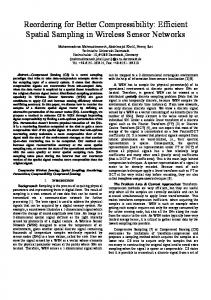
Fig. 1: (a) BioBiped2 robot used in the example application in Sec. II (6 degrees of freedom, mass: 11.5 kg, hip height; 0.7 m). (b) Kinematic structure highlighting the relevant active TD-SEAs with motor and spring (Soleus (SOL), Vastus (VAS)) and passive (Gastrocnemius (GAS)) structures. (c) Definition of the GAS rest angle α and the GAS attachment point numeration 1 to 6.

to mechanical systems by using series elastic actuators, which can passively reduce peak forces. Further, they can be used to store and release energy to make a cyclic gait more efficient by making the overall leg act as a spring. Implementing the actuation in a musculoskeletal arrangement, using tendon driven series elastic actuators (TD-SEAs) connected to the joints in an antagonistic setup, further advantages seen in humans can be exploited. The biarticular structures can help to synchronize the joint motions to avoid overextension of individual joints, increasing the robustness of the overall leg motion [13]. Also, their ability to transfer energy from proximal to distal joints can be utilized to design more lightweight extremities. The BioBiped2 robot (see Fig. 1 and www.biobiped.de) which uses TD-SEAs for its joint extensors with passive springs as antagonists and biarticular structures is used in the example application in Sec. II. This robot is the second generation robot based on the insights gained from the BioBiped1 platform described in [12]. It is also the first to which the approach proposed in this paper is being applied. Hardware improvements over the first generation include ball bearings in the joints, lower gear ratios for higher rope speeds and a modular electronics design to allow the use of more sensors and actuators depending on the current motion goal. To achieve a desired motion on such a musculoskeletal robot a number of parameters in hardware and software influencing the passive and active dynamics and control properties have to be designed and properly tuned. Using

detailed multi-body system dynamics models like for conventional rigid robots is an even more difficult process for musculoskeletal robots. The highly elastic structures of the TD-SEAs, the dynamic interplay between multiple links and joints through biarticular structures and changing interaction with the ground during dynamic bouncing motions make a sufficiently accurate modeling of musculoskeletal robot dynamics highly difficult. Differences between simulation model and hardware that are non-trivial to remove include among others the non-linearities of physical springs, the unknown friction in joints and the modeling of the ground contact [7]. Therefore, optimization of these parameters only by robot dynamics simulation is not sufficient. On the other hand using the actual robot in a hardwarein-the-loop optimization to find the best parameter values is very expensive with respect to time and can also be harmful to the robot hardware prototype. The number of robot experiments needed for the optimization depends on the number of parameters involved. In musculoskeletal robots the addition of elastic elements and biarticular structures increases this number compared to rigid robots. Each experiment has a wear on the robot’s hardware, which restricts the number of experiments possible. Further, the time needed for manually modifying hardware parameters, like spring stiffness or lever arm length, makes each experiment costly. Damaging the hardware through use of unsuitable parameter combinations adds to the cost of the robot experiments in terms of repair time. Therefore, a new approach is presented to reduce the costs of optimizing design and parameter tuning of musculoskeletal robots. The number of robot experiments needed is reduced through systematic interpretation of results of specifically designed simulation experiments. Furthermore, parameter combinations are excluded which are possibly harmful to the hardware and by sequencing the experiments to have fewer hardware modifications in between them. A. State of the Art Design and tuning of elastic musculoskeletal bipedal robots has been described by Hosoda et al. [5], [8] and Niiyama et al. [9], [10]. In [5] the design, tuning and motion generation of a pneumatic biped which performs jumping, walking and running motions is described. The motion parameters are manually tuned for each of the motions performed without the use of simulation or optimization methods. In [8] inertial measurement sensors in the trunk of the robot are used to detect its roll angle for stabilization of a rebound motion. Since the experiments are performed only on the hardware without help of simulation models, hundreds of trials on the robot are needed to collected sufficient data. While in [10] a simulation model is used to adapt human muscle activation patterns to the Athlete robot simulation model, the resulting parameters are still manually tuned on the robot afterwards. In [12] the BioBiped1 musculoskeletal robot performs synchronous and alternate hopping motions using a manually

Fig. 2: Overview of the steps performed in the optimization process.

tuned parameters. All mentioned approaches, as well as the experiments carried out on BioBiped versions 1 and 2 so far, used robot parameters manually tuned directly on the hardware without systematic exploitation of simulation results. II. E XPERT G UIDED O PTIMIZATION BY E XAMPLE The goal of this work is to efficiently determine a parameter configuration for possibly optimal motion of the robot while keeping the number of hardware experiments and the time consumed by performing them low. To find the optimal values for the relevant motion parameters a hardware-inthe-loop optimization is performed which is guided by a human expert. This expert reduces the number of hardware experiments by applying knowledge about the robot’s behavior gained from previous experiments, biomechanical understanding of the system, and interpretation of results from simulation experiments. As the knowledge from previous experiments and the biomechanical understanding are difficult to exploit in a systematic and reproducible manner, this work will focus on the systematic generation, interpretation and usage of the simulation results. This approach is split into the four steps shown in Fig. 2 which are detailed in the following sub-sections. The approach is applied to the musculoskeletal bipedal robot BioBiped2 shown in Fig. 1, which uses TD-SEAs based on DC-motors, synthetic ropes and metal extension springs as actuators. For the simulation experiments a multibody system (MBS) simulation model is used, that was developed for the BioBiped robot series in [11]. The overall goal of the BioBiped project is to perform different gaits on a single robot configuration from jogging to walking to stable standing. As first step towards jogging with this new robot model, hopping is considered. The performance of a synchronous hopping motion, including impacts and push-offs, is optimized here as a prerequisite for future jogging motions. While in this robot multiple biarticular structures can be attached, in this example only the bi-articular GAS is used because of its relevance for the considered hopping motion. A. Definition of Motion Goal and Optimization Settings The motion goal needs to be defined including a quality criterion which can be measured or derived for both the simulation and the hardware experiments. Using the human leg

as model, the biomechanical understanding of its functional structures is used to identify which of the robot’s structures are relevant for the selected motion goal. The goal of the example optimization is to improve the hopping performance in a synchronous hopping motion. From biomechanics it is known, that human hopping is primarily powered by ankle motion [2]. Therefore, the mechanical structures in the BioBiped2 robot most relevant for this motion are the active mono-articular ankle extensor SOL and the passive bi-articular GAS. So the parameters p subject to the optimization performed in this example application are the stiffness of the SOL and GAS structures as well as the rest length and lever arm of the GAS. For the SOL and GAS stiffness five different springs are available with their parameters listed in Tab. I. The GAS structure has a fixed lever arm length on the thigh and six possible attachment points at the heel (shown in Fig. 1c) with their distance from the center of the joint listed in Tab. I. Its rest length is the only continuous parameter which is described through the knee and ankle angles corresponding to its rest position. This is the most practically viable approach on the robot, since both joints feature position encoders, which can be used to measure the currently set rest length. Positioning the knee joint at 45 deg bent from full extension the adjustable GAS rest length corresponds to ankle joint angles between 0 deg and 40 deg bent from center position. This GAS rest angle α is defined as shown in Fig. 1c (with the SOL disengaged). The objective of the optimization is to minimize the quality value q ∈ R. It depends on the vector of design parameters p, which may include real- and integer-valued parameters and which are to be tuned by the expert guided optimization approach. The quality q of the hopping is calculated from the duty factor qdf and the maximal center of mass (CoM) height qcom as shown in Eq. (1). The CoM position is located in the lower trunk in straight standing, which is used as the fixed reference point for the hopping height measurements q(p) =

qˆdf (p) + qˆcom (p) . 2

(1)

Using just one of them for the quality might allow for non-hopping motions to achieve good quality values, e.g. by just pulling up the feet for a low duty factor or just standing on fully extended legs for a high CoM height. The combination of both ensures an actual hopping motion with flight phase and upward motion of the CoM. To ensure an equal weight of both parts they are normalized based on the minimal and maximal values found in the simulation min max coverage experiments: qˆdf (p) = (qdf (p) − qdf )/(qdf − min min max min qdf ), qˆcom (p) = (qcom (p) − qcom )/(qcom − qcom ). Also, to formulate this as a minimization problem qcom is set to the negative maximal CoM height of one motion cycle. The values of the two parts are calculated as shown in Eq. (2): qdf (p) =

tstance , qcom (p) = −hmax tstance + tflight

(2)

Attachment point Distance [mm] Spring constant [N/m] Force limit [N]

1 45.3

2 51.1

4100 162.8

3 56.8

7900 341.5

4 62.7 10000 356.7

5 68.5 13000 341.5

6 74.5 15600 386.7

TABLE I: Parameter values of the available attachment points and springs.

In simulation the maximal CoM height hmax can be directly read from the model as the highest point of the CoM trajectory during flight phase. For the robot experiments this value is calculated as a combination of accelerometer and kinematic data. The vertical position of the trunk is calculated from the measured joint angles via forward kinematics during ground contact and the accelerometer data is used to calculate the trajectory during the flight phase. The drift of the accelerometer is compensated using the heights of the trunk known from the kinematics just before and after the flight phase. The ground contact forces are used to divide the motion into stance and flight phase for both the simulation and the robot. The duty factor qdf is calculated as stance time tstance in relation to the time of a hopping cycle tstance + tflight . A minimal vertical force value of 10 N is used to detect ground contact for the simulation and the robot to ensure equal calculations for both. As safety criterion for the robot the maximal forces fmax , that occur at the actuation structures for SOL, GAS and VAS, spring are compared to the force limit flimit of the spring currently used in the respective structure on the robot which can be seen in Tab. I. Configurations where the limits of any of the three springs are exceeded as shown in Eq. 3 are marked in the visualization and excluded from the robot experiments to protect the mechanics. spring x fmax > flimit ,

x ∈ [SOL, GAS, V AS]

(3)

While hopping, the robot is stabilized by an external mechanism constraining its trunk motion to vertical translation. The hopping is performed on flat ground and the motor power supply is limited to maximal output of 10 V to protect the system. The motion trajectory is generated by a state machine with two states switching between a bent and an extended leg configuration. Transitions between the two states are triggered by the ground contact events touchdown and liftoff and trajectory transitions are smoothened by a spline interpolation from the current actuator positions to the new goal positions. The tracking of the trajectories is performed by a motor position controller with the same manually tuned gains in simulation and on the robot. Initially the robot is in the bent configuration and is dropped manually from a height with 5 cm ground clearance. B. Design of Simulation Experiments The simulation experiments are designed to achieve three goals: • Understanding the sensitivity of the quality criterion, • Recognizing correlations of multiple parameters,

For the first two goals a coverage of the parameter space is needed and for the third an optimization in simulation is used to find a good starting point. To achieve a good coverage of the parameter space with the simulation in feasible time the continuous parameter GAS rest angle is discretized into nine values. Together with the three discrete parameters this results in a total number of parameter configurations for the coverage simulation experiments of 9 ∗ 5 ∗ 5 ∗ 6 = 1350. With an average of 10 s needed to simulate the experiment for one configuration the approximate total time needed for simulation is 3h 45m, which allows for a full factorial design of experiments [1]. To optimize the continuous parameter this nonlinear function with continuous and discrete variables a mixed-integer nonlinear problem (MINLP) has to be solved without gradient information. A surrogate based mixed-integer nonlinear black box optimization is chosen [3], which can make use of the already extensive data gained in the coverage experiments as initial data set for its surrogate function. C. Visualization and Interpretation of Simulation Results The goal in this step is to systematically leverage the results from the simulation experiments to help plan the robot experiments to be as efficient as possible. Mapping the simulation results to the robot results is difficult to automate, since the model error of the simulation and any inaccuracies in setup of the hardware are not known. Results from the robot experiments could be used to improve the simulation accuracy, but this is beyond the scope of this work. Therefore, a systematic approach is used to leverage the knowledge gained by interpreting the simulation results with the help of visualization of the quality criterion. As the parameter space has four dimensions plus the dimension of the quality criterion the visualization has to be split into multiple plots. A two dimensional grid of two dimensional plots was chosen with the quality criterion represented through color as can be seen in the overview Fig. 3. Due to space constraints only a subset of the parameter space is visualized in more detail in this publication. For the reduction of the parameter space three plots showing different sectional planes through the optimal configuration found in simulation are shown in Fig. 4. 1) Exclusion of harmful parameter configurations: As can be seen in the overview Fig. 3 and in the detailed plots in Fig. 4 only a few harmful configurations, marked as magenta diamonds, were identified in simulation based on Eq. (2). These configurations lead to maximal forces in one of the three elastic structures of SOL, GAS or VAS that were higher than the specified force limit of the springs to be used on the robot. To protect the robot from damage, these configurations will be excluded from the robot experiments. 2) Adjustment of the quality criteria visualization boundaries: The upper boundary for the quality criterion is set to 0.7 in the visualizations shown in this paper. This value was manually selected by the expert to focus on the relevant area

15600 13000 10000 7900 4100 15600 13000 10000 7900 4100 15600 13000 10000 7900 4100 15600 13000 10000 7900 4100 15600 13000 10000 7900 4100

0.65 0.6 0.55 0.5 0.45

quality

Selecting a starting point for the robot experiments. SOL stiffness [N/m]

•

0.4 0.35 0.3 0 10 20 30 40 0 10 20 30 40 0 10 20 30 40 0 10 20 30 40 0 10 20 30 40 0 10 20 30 40 GAS rest angle [deg]

Fig. 3: An overview of the results gained through the simulation coverage experiments spread over the parameter space. All plots show the same sectional plane of the parameter space with the GAS rest angle on the x-axis and the SOL stiffness on the y-axis. The plots in each column share the same GAS attachment point 1 to 6 from left to right. The plots in each row have the GAS stiffness in common, with the lowest spring coefficient in the top and the highest in the bottom row. A more detailed excerpt of the plot with the best value can be found in Fig. 4a. (black circles: simulation experiments colored with quality values (best values are dark blue), magenta diamonds: harmful configurations, green circle in bottom row second column: the best value found)

of the parameter space and clearly show the differences in the quality around the optimal value as can be seen in Fig. 4. 3) Exclusion of parameters: In Fig. 4b it can be seen that the stiffness value of the GAS structure has only a very small influence on the quality criterion, but cannot completely be excluded from the optimization. 4) Recognition of parameter correlations: By visualizing all sectional planes of the parameter space as shown in Fig. 4, linear correlations between all parameter combinations can be visually inspected. In this example application, a linear correlation is only found between GAS rest angle and GAS attachment point as shown in Fig. 4c. This information is used in the next section when planning the robot experiments. D. Expert Guided Robot Experiments Based on the interpretation of the simulation results the robot experiments can now be planned and executed in a more efficient manner. 1) Design for the initial robot experiments: First a start configuration for the robot experiments has to be selected. Based on the simulation results, it is safe to use the optimal configuration found in simulation, as no harmful configurations are close to it. The initial robot experiments are planned around the start configuration varying each parameter by a single step in both directions as proposed in [1] with the central finite differencing approach described in [1]. The step size is chosen for the discrete parameters to be one step and for the continuous GAS rest angle to be the size of its discretization. As these step sizes show significant changes in the quality criterion, this will give the expert a first impression of the gradients of each parameter on the robot and allow for a visual mapping between simulation and robot results. 2) Execution and further selection of robot experiments: After the seven initial experiments, the results are visualized, shown in the top left plot in Fig. 5a entitled ’experiment 7’.

10000 7900 4100 0

5 10 15 20 25 30 35 40 GAS rest angle [deg]

15600

6

13000

5

10000 7900 4100 5 10 15 20 25 30 35 40 GAS rest angle [deg]

0.65 0.6 0.55 0.5

4

0.45

3

0.4

0.35

2

0.3

1 0

0.7

quality

13000

SOL stiffness [N/m] 15600 GAS stiffness [N/m] 15600 GAS attachment

GAS stiffness [N/m]

SOL stiffness [N/m]

15600

SOL stiffness [N/m] 15600 GAS attachment 2

better

GAS stiffness [N/m] 15600 GAS attachment 2

0

5 10 15 20 25 30 35 40 GAS rest angle [deg]

(a) The strongest influence on the quality cri-

(b) The stiffness of the GAS structure has

(c) A correlation can be seen between the rest

terion is the rest angle of the GAS structure, but also the stiffness of the SOL is relevant.

very small influence on the quality criterion in the area with good results colored in blue.

angle and the attachment point of the GAS structure.

Fig. 4: Three different sectional planes of the simulation results cut through the best configuration. (black circles: simulation experiments colored with quality values, magenta diamonds: harmful configurations, green circle: the best value found)

Here it can be seen, that the best configuration so far (marked with a green circle) has a lower SOL stiffness than the optimum found in simulation (marked with a purple square). Following the gradient in the quality value towards the next lower SOL stiffness value reveals an even better result in ’experiment 8’. By following this gradient further along the SOL stiffness and GAS rest angle parameters a local optimum is found in ’experiment 10’. As the visualization after ’experiment 12’ shows that the SOL stiffness parameter N set to 10000 m leads to the best results in this sectional plane, the search is continued in the sectional plane between GAS attachment point and GAS rest length shown in Fig. 5b. Due to the linear diagonal correlation found in this plane in the simulation experiments, neighboring configurations along this correlation are tested in experiments 13 and 14 as shown in Fig. 5b. In experiments 15 and 16 more fine grained changes of 2 deg to the continuous GAS rest angle parameter are tested with no further improvement of the quality criterion. With experiments 17 to 19 all direct neighbors of the best configuration found so far are tested. 3) Termination of the robot experiments: The termination criterion used in this example application is the confirmation of a local optimum. To ensure a local optimum also the neighboring values along the parameter correlation found in simulation between GAS rest angle and GAS attachment point have been tested. E. Comparison to Surrogate Based Optimization Method To be able to evaluate the proposed approach, a conventional hardware-in-the-loop optimization is applied to the example application for comparison. The optimization problem is formulated as a minimization problem using the quality criterion q as described in Eq. (1). Additionally, the safety criterion described in Eq. (3) is used based on the simulation data to identify harmful configurations before they are tested on the robot. When the optimization chooses to evaluate such a harmful configuration, it is not performed on the robot, but marked as infeasible for the optimization. The optimization terminates, when the quality criterion converges or the number of robot experiments after the initial design

is twice that of the expert guided approach, namely at experiment 31. The optimization has to be performed with a problem solver capable of handling mixed-integer nonlinear problems. A surrogate based mixed-integer black box optimization approach (SurOpt) [3] has been shown to find good parameter configurations with a low number of hardware experiments for related problems [4]. Therefore, it is a valid candidate for comparison with the expert guided approach presented in this work. The parameters to be optimized are the same as in the expert guided approach: SOL stiffness, GAS stiffness, GAS attachment point and GAS rest angle. The ranges of these parameters are normalized to be mapped to the ranges from 0.0 to 1.0 to allow for an efficient search in all parameter dimensions. A branch and bound approach is used to handle the three discrete parameters. A distance based update criterion is used in this optimization (compare [3], Chapter 4.2), which enforces a minimal distance  between tested configurations. The value of  is chosen to be 0.025, corresponding to changes in the GAS rest angle of 1 deg, which is the minimal change that is practically feasible on the robot. As suggested in [3], expert’s guesses are used for the initial design points. Here the optimization is started on the robot with the same initial design around the simulation optimum. Sequential updates to the parameter configuration are selected by the optimization algorithm to either improve the quality criterion or the surrogate function mean square error as described in [4]. The configurations are tested on the robot and evaluated in the same manner as for the expert guided experiments making the resulting quality values directly comparable. The optimization found the same solution as the expert guided approach after 28 robot experiments, but its termination criterion of converging results was not yet fulfilled. After 31 experiments the optimization was stopped with the maximum number of experiments defined as second termination criterion.

experiment 8

experiment 9

experiment 10

experiment 11

experiment 12

0.7

experiment 19

0.65

13000 10000

0.6

7900 4100

0.55 25

30

35

40 25

30

35

40 25

30

35

40 25 30 35 40 25 GAS rest angle [deg]

30

35

40 25

30

35

40 25

30

35

40

0.5

N (a) The graphs show the plane with GAS stiffness fixed at 15600 m and GAS attachment in position 2. After the seven initial robot

experiments around the start configuration, the gradient is followed in experiments 8 to 12 to find the best values for the stiffness of SOL and the rest angle of GAS. experiment 14

experiment 15

experiment 16

experiment 17

experiment 18

experiment 19

0.45 0.4

3

0.35

better

GAS attachment

experiment 13

quality

SOL stiffness [N/m]

experiment 7 15600

2 1

0.3 25

30

35

40 25

30

35

40 25

30

35

40 25 30 35 40 25 GAS rest angle [deg]

30

35

40 25

30

35

40 25

30

35

40

N N and SOL stiffness fixed at 10000 m . In experiments 13 and 14 (b) The graphs show the plane with GAS stiffness fixed at 15600 m

the attachment point and rest length of GAS were optimized by first testing the two points along the diagonal correlation of the two parameters known from the simulation results (Fig. 4c). Then in experiments 15 and 16 the continuous rest angle of GAS was modified more fine grained than in the discretized steps used before. Finally, in experiments 17 to 19 the best configuration found so far was confirmed to be at least a local optimum.

Fig. 5: Iterative construction of the visualization for the results of the robot experiments. Markers show the best configuration from simulation as purple square, the best configuration on robot so far as green circle and the newly added result as red star.

F. Discussion of Results

experiments (SurOpt) best value (SurOpt)

0.44

quality

0.42

better

The best parameter configurations p found by manual tuning, the simulation optimization, the expert guided approach and the SurOpt optimization with their corresponding quality values q(p) and maximal CoM heights evaluated on the BioBiped2 robot are listed in Tab. II. The quality from the manually tuned result of 0.443 is improved already by using the optimal configuration found in simulation on the BioBiped2 robot which leads to a quality value of 0.375. Further improvement was possible using the expert guided approach and the SurOpt hardware-in-the-loop optimization, both resulting in the same optimal configuration with a quality of 0.342. While the expert guided approach and the SurOpt optimization both find the same optimal configuration the former needs fewer robot experiments as shown in Fig. 6. It can be seen that it took SurOpt 28 experiments to find this optimum while the expert found it on the 10th experiment. To better understand the results the quality value can be split into its two parts, the maximal center of mass height qcom and the duty factor qdf . While the quality improvement through the simulation stems from both the maximal CoM height and the duty factor, the improvement made in the robot experiments comes from an increased maximal CoM height. Compared to the manually found configuration the optimal configuration found in simulation already results in an improvement of the maximal CoM height of 12 mm.

experiments (expert guided) best value (expert guided)

0.4 0.38 0.36 0.34

5

10

15 20 experiment number

25

30

Fig. 6: Comparison of the quality criterion value over the course of the expert guided and SurOpt optimization robot experiments. It can be seen that the same seven initial configurations have been used on both approaches. Afterwards the expert guided approach improves the quality criterion much quicker and finds the best solution in experiment 10 while SurOpt finds the same configuration only in experiment 28.

But the optimal solution found by both the expert guided and the SurOpt optimization gives an even higher gain of 22 mm while the duty factor is almost the same as found through simulation. III. C ONCLUSION This work introduces a systematic approach to optimize parameters of a musculoskeletal bipedal robot efficiently

SOL GAS attach- rest stiffness stiffness ment angle [N/m] [N/m] point [deg] manual tuning simulation expert guided SurOpt

results q

qcom [m]

qdf

num. robot experiments

For such robots with biomechanically inspired elasticity and damping properties, optimally balancing passive and active dynamics and control properties through parameter tuning is less effective with existing approaches.

15600

7900

3

30

0.443 0.783 0.383

14

15600

15600

2

30

0.375 0.795 0.352

0

ACKNOWLEDGMENT

10000

15600

2

35

0.342 0.805 0.354

19

10000

15600

2

35

0.342 0.805 0.354

31

This research has been supported by the German Research Foundation (DFG) under grant no. STR 533/7-2. The authors would like to thank Katayon Radkhah for providing highly capable BioBiped simulation models [11] and Stefan Kurowski for helpful discussions.

TABLE II: Shown are the parameter configurations p for the best (minimal) quality values q(p) found with manual tuning, the simulation optimization, the expert guided approach and the SurOpt optimization. The resulting quality values were produced on the BioBiped2 robot. The number of robot experiments needed to find these configurations are listed in the last column.

by reducing the number of needed hardware experiments through exploitation of simulation results. By systematic interpretation of the simulation results an expert can plan the hardware experiments to be more efficient than a stateof-the-art hardware-in-the-loop optimization method. A parameter optimization of the musculoskeletal BioBiped2 robot to increase hopping performance was used as an example application to compare this new approach with a state-of-the-art hardware-in-the-loop optimization method. The parameters selected for optimization all had significant influence on the quality criterion, except for the stiffness of the GAS. As the quality criterion is a performance criterion which reflects the hopping height of the musculoskeletal robot, this can be explained through the biomechanical understanding of the role of the GAS structure. Its main purpose is to distribute power between the knee and ankle joints and not to store and release energy in its elastic element. Therefore, its elastic property is not as important for the quality criterion when compared to its other two parameters, rest length and lever arm, which shape the kinematics of the power transfer. The other two parameters of the GAS (lever arm length and rest length) showed significant influence on the hopping performance. As the role of the GAS in human locomotion includes powering the push-off of the leg before the swing phase, it can be concluded that optimizing its parameters is important to improve the locomotion performance. In this example application the newly presented expert guided approach needed a total number of 19 hardware experiments to find and validate the optimal configuration. While the state-of-the-art optimization method found the same solution, 31 experiments were needed and no validation of it to be at least a local optimum was included. Further, through the expert guided sequencing of the experiments less time was needed for the hardware modification between experiments. In total the newly presented approach needed only 61% of the robot experiments and 52% of the time for the experiments and hardware modifications compared to the other optimization method while finding the same result. Although the presented approach can be applied to general robot designs as well, it is expected to be most beneficial for highly complex robot designs such as musculoskeletal robots.

R EFERENCES [1] R.C.M. Brekelmans, L.T. Driessen, H.J.M. Hamers, and D. den Hertog. Gradient estimation schemes for noisy functions. Journal of Optimization Theory and Applications, 126(3):529–551, 2005. [2] C.T. Farley and D.C. Morgenroth. Leg stiffness primarily depends on ankle stiffness during human hopping. Journal of Biomechanics, 32(3):267–273, 1999. [3] T. Hemker. Derivative Free Surrogate Optimization for Mixed-Integer Nonlinear Black Box Problems in Engineering. PhD thesis, TU Darmstadt, Germany, 2008. http://tuprints.ulb.tu-darmstadt.de/2162/. [4] T. Hemker, M. Stelzer, H. Sakamoto, and O. von Stryk. Efficient walking speed optimization of a humanoid robot. International Journal of Robotics Research, 28(2):303 – 314, 2009. [5] K. Hosoda, T. Takum, A. Nakamoto, and S. Hayashi. Biped robot design powered by antagonistic pneumatic actuators for multi-modal locomotion. Robotics and Autonomous Systems, 56(1):46–53, 2008. [6] S. Kajita, T. Nagasaki, K. Kaneko, K. Yokoi, and K. Tanie. A running controller of humanoid biped HRP-2LR. In Proc. IEEE Intl. Conf. on Robotics and Automation, pages 616–622, 2005. [7] T. Lens, K. Radkhah, and von Stryk. Simulation of dynamics and realistic contact forces for manipulators and legged robots with high joint elasticity. In Proc. Intl. Conf. on Advanced Robotics, pages 34– 41, 2011. [8] X. Liu, A. Rosendo, M. Shimizu, and K. Hosoda. Improving hopping stability of a biped by muscular stretch reflex. In Proc. IEEE-RAS Intl. Conf. on Humanoid Robots, pages 658–663, 2014. [9] R. Niiyama and Y. Kuniyoshi. Design of a musculoskeletal Athlete robot: A biomechanical approach. In Proc. Int. Conf. on Climbing and Walking Robots, pages 173–180. World Scientific Publ., 2009. [10] R. Niiyama, S. Nishikawa, and Y. Kuniyoshi. Athlete robot with applied human muscle activation patterns for bipedal running. In Proc. IEEE-RAS Int. Conf. on Humanoid Robots, pages 498–503, 2010. [11] K. Radkhah. Advancing Musculoskeletal Robot Design for Dynamic and Energy-Efficient Bipedal Locomotion. PhD thesis, TU Darmstadt, Germany, 2014. http://tuprints.ulb.tu-darmstadt.de/3934/. [12] K. Radkhah, C. Maufroy, M. Maus, D. Scholz, A. Seyfarth, and O. von Stryk. Concept and design of the BioBiped1 robot for human-like walking and running. International Journal of Humanoid Robotics, 8(3):439–458, 2011. [13] D. Scholz, C. Maufroy, S. Kurowski, K. Radkhah, O. von Stryk, and A. Seyfarth. Simulation and experimental evaluation of the contribution of biarticular gastrocnemius structure to joint synchronization in human-inspired three-segmented elastic legs. In Int. Conf. on Simulation, Modeling and Programming for Autonomous Robots, pages 251–260, 2012. [14] A. Seyfarth, K. Radkhah, and O. von Stryk. Soft Robotics - Transferring Theory to Application, chapter Concepts of Softness for Legged Locomotion and their Assessment, pages 120–133. Springer Verlag, 2015.