A fault tree for a dangerous failure is shown in figure. 2. The names of the basic events are composed of the failed component and the kind of failure. For a more.
Efficient Generation and Representation of Failure Lists out of an Information Flux Model for Modeling Safety Critical Systems Michael Pock1,2,4, Hicham Belhadaoui1,3,4, Olaf Malass´e1 & Max Walter2 1) Arts et M´etiers Paristech, Metz 2) Technische Universit¨at M¨unchen 3) ENSEM Casablanca 4) Centre de Recherche en Automatique de Nancy
This article presents a new way to model safety critical systems hierarchically. An information flux diagram as high level and finite automatons as low level model are combined. With these models, scenarios leading to dangerous failures as well as spurious trips can be generated. Furthermore, we will show how to extract the different scenarios out of the model in a very efficient way using different BDD-techniques. Finally, a theoretical complexity analysis for the used algorithms is given.
prevent any accident. But Fault Trees are just boolean models, every event or component can only have two modes. Furthermore they cannot model dependencies directly which will occur between different kind of failures. There are also two unwanted events for the global system, while fault trees are just capable to model one single event. So it would be necessary to create two models with a lot of common components and events. Petri Nets in contrary are more powerful. There is no limitation to the number of states of a component, and it is possible to calculate several events in one PN. But they are not very intuitive. They also cannot be created hierarchically, as a small change in one component will affect the whole PN. This is the reason that we will present a powerful high-level model which can handle all these specific problems for safety-critical systems, based on the theoretical work of Karim Hamidi (Hamidi 2005) in section 3. An efficient solution method will follow in section 4. At the moment, there is no implementation of the presented algorithms, though. So we only will present some theoretical results of the expected performance in section 5.
1 INTRODUCTION A serious problem for the design and evaluation of safety critical systems, for example used in the automation domain, is to forecast the safety of the system. It’s not possible to measure it for two reasons. At first, normally these accidents should occur very rarely, so that a system has to run for a very long time to get reasonable results. Furthermore, it is very questionable to run a safety-critical system which can cause a lot of harm without knowing anything about its dependability. So the only solution is to use a model to evaluate the safety of the system. Another problem are unspecificated activations of safety functions, the so called spurious trips. They can lead to the unavailability of the system and cause extra costs. Furthermore, too many spurious trips can be dangerous as well. If there are too many false alarms or shutdowns, the operators and surrounding people could start to ignore the alarms or try to prevent the shutdowns, even if there is a dangerous situation this time. Currently, mainly standard models like fault trees (Lee et al. 1985) and Petri nets (Leveson and Stolzy 1987) are used. Fault trees are easy to use, but they have several limitations. At first, components in safety critical systems often have more than one failure mode. They can create dangerous failures or spurious trips itself and propagate these to other components. They even can prevent specific failures of other components. For example, an unwanted shutdown will
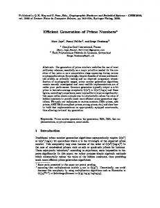
2 AN EMERGENCY STOP SYSTEM To illustrate the presented model, the emergency stop system of a chemical reactor (Figure 1) will be used which is described in this section. This system should stop the reaction if the temperature in the reactor is 1
Figure 2: The fault tree for the dangerous failure of the emergency stop system the shutdown was successfull. For this system, there are two possible kinds of failures in general. Either the emergency system is not available (dangerous failure), or it shuts down the system in a safe state leading to a unneccessary unavailability of the whole reactor. (spurious trip) A failure of the whole emergency system can be caused by several different failures of its components. We will classify these failures as dangerous (D), nondangerous (S) or lost inhabitant (I), which means that the component does not have an output. The sensors can either measure a value which is too high (S), too low (D), or return no value at all (I). The input modules can either lose the data of the sensors (I) or change it to a higher (S) or lower (D) value. In the memory the stored data can be distorted by a bitflip in either a dangerous (D) or nondangerous (S) way. It can happen that the watchdogs don’t detect a missing input (D), or that they report such a missing input although there was one (S). The control unit can decide to start a shutdown in a safe state (S) or to not start a shutdown in a dangerous state (D). The output modules can fail to give the orders to their motors to close the valves (D), while the motors can fail to start (D). Finally, the valves can be blocked in an open (D) or closed (S) position. It’s possible to discriminate the single components further, but in this section we will limit our explana-
Figure 1: A emergency stop system of the chemical reactor getting too high by stopping the inflow of the chemicals. The sensors S1 and S2 measure the current temperature of the chemicals in the tank and transport their results to the controller. The controller reads this result via his inputs In1 and In2 and will store these values for synchronization in its memory. (St1, St2). To avoid a loss of information, the watchdogs W d1 and W d2 control the inputs. Afterwards, the V oter decides, if there is a dangerous situation. If after the voting process the control unit CU decides to shut down the system, this information is proceeded to the output modules Out1 and Out2 and passed to the motors M1 and M2 which get the order to close the valves V 1 and V 2. If at least one of these valves is closed, 2
tion on the general outline of the system. A fault tree for a dangerous failure is shown in figure 2. The names of the basic events are composed of the failed component and the kind of failure. For a more detailled analysis, the basic events could be replaced with subtrees. This fault tree has some problems though. At first, some basic events for the same components, but for different failure modes are stochastically dependent. Furthermore, some component failures will prevent a dangerous failure of the whole system, for example a blocked valve in its closed state. These effects can not be included directly in the fault tree.
transformation of information. The last type of blocks are DEC-blocks. They represent logical decision entities. They have several inputs and one output, and describe the behavior of multiple interconnected sources of information. They don’t describe any physical entities. The components which make this decision have to be included by adding a successing ST-block. One block in the diagram, normally a ST- or DECblock, can be marked as final block. This block has no output and is used to generate the failure scenarios which will be described in section 3.4. An example of an IFD for the given example in section 2 is shown in figure 3 There are blocks for the different modules of the system, and some extra decision blocks. Lost1 and Lost2 decide, if the signal of the sensor is lost, CD decides if the voter will get the necessary inputs for a correct voting and Saf e is used for the final decision if there is a dangerous failure or a spurious trip. The information flows from the source blocks to the final block in one general time step t. In the source blocks, the sensors create the information which will flow through our diagram. This information proceeds to the successing blocks where it is processed and proceeded further. The exchange between the blocks always works faultless. While processing the data in the blocks, faults can occur or be detected. This means, that the state of signal can change within a block. We distinguish three different erreonous states for the signals:
3 THE INFORMATION FLUX MODEL We are mainly interested in two different events of the system: • Dangerous incidents which could lead to accidents • Non-dangerous spurious trips We want to extract all scenarios leading to one of these two undesired events of the whole system. To model these we use a directed block diagram representing the information flux through the system for high level and finite state automatons and rules for low level modelling. This information flux diagram (IFD) and the automatons are generalized versions of the diagrams and automatons presented in (Hamidi 2005).
• A non-existent failure has been detected. (Safe failure state S) • An existent failure has not been detected. (Dangerous failure state D)
3.1 Information Flux Diagram For the IFD, we use different kinds of blocks which represent different functional entities. We distinguish:
• The signal is lost. (Inhabitant failure state I).
• WD-blocks for watch dogs
3.2 Finite automatons After modeling the information flux it is necessary to specify the state changes of the information. For non-DEC-blocks finite, acyclic automatons are used. A finite automaton (Brookshear 1989) is a quintuple (X, Y, f, x0 , Xf ) with
• SRC-blocks as sources of information • DEC-blocks for logical decisions • ST-blocks for all other functions (storage of information, transformation of information, selftests etc.)
• a finite set of states S • an input alphabet Σ
Blocks of the type WD are used specially for control units with a watch dog. They have one input and one output and can detect the absence of sensible information in order to react accordingly afterwards by forwarding default or special error values. SRC-blocks create the information which flows through the diagram. They represent the sensors in the system and have only one output. ST-blocks are the most versatile blocks. They have one in- and one output, and they are used for all functional entities which cannot be represented by the other blocks, e.g. the storage or the
• a transition function δ : S × Σ → S • a nonempty set of initial states S0 ⊂ S • a set of final states F ⊂ S For our example, we have one predefined initial state x0 , possibly other initial states and three predefined final states xS , xD , and xI which represent the three faulty states of information. The used alphabet in 3
Figure 3: The IFD for the emergency stop system indicates the state of the hardware resource x: working correctly (0), non-dangerous failure (S), potential dangerous failure (D) or no output (I). bf (e) represents environmental errors like bit flips of a resource e. f t(f ) indicates that a testing resource f has not detected an error. To simplify the calculation, we assume that the state of a hardware-, bit flip- or fault test-resource is always the same in one time step. Note that all three final states are not always needed. Only final states which can be detected by the inits of the successor blocks have an influence on the result and are necessary. This will be explained more detailed in the next subsection. The automatons define a language which describes all scenarios leading to the different failures of the block. We can distinguish three different sub languages for non-dangerous failures, potential dangerous failures and failures with no output. These languages can be extracted and are saved in the three lists LS (B), LD (B), and LI (B) for the block B.
these automatons are symbols which represent different kind of failures. They are denoted as follows: • init(i) with i ∈ {S, D, I} (For ST- and WDblocks) • d(x, y) with x as a hardware resource and y ∈ {0, S, D, I} • bf (e) with e as bitflip resource • tf (f ) with f as testing resource • The empty word ǫ
3.3 Rules of DEC-blocks Decision blocks use another low level model to describe their behavior. For this purpose, boolean rules are introduced. These rules use the state of the signals (either S, I or D) of each input. There are three rules, they represents the lists LS , LD and LI . If we take a look at the final block of the IFD shown in 3, the following rules are chosen: S :V1=S∨V2=S D : V1 = D∧V2 =D I : f alse So, the final block will create a spurious trip if at least one of the two valves will create one. A dangerous failure will only occur if both valves will fail dangerously. As we are searching a complete list, we have to define how to extract it. Disjunctions in the rules will be handled by unifying two lists, Conjunctions will be handled by set products. For the given example we can conclude: LS (Saf e) = LS (V 1) ∪ LS (V 2) LD (Saf e) = LD (V 1) × LD (V 2) LI (Saf e) = {}
Figure 4: The Automaton for the block Store1 An example, the automaton for the block Store1, is shown in figure 4. While storing the results, different failures can occur. At first, the memory mem can be damaged physically, so that there are several bits which are locked to one (S), locked to zero (S) or the memory is not available at all (I). There is also the possibility of a bitflip in the memory, changing the value of the stored data. init(i) is used for the fault propagation of the predecessor block. It only occurs at the initial state x0 . The possible values for i depend on the type of the current block. In ST-blocks, i can only be S or D as ST-blocks aren’t capable of handling lost information. By contrast, WD-blocks only contain init(I). For hardware failures, the symbol d(x, y) is used. y 4
nary Expression Diagrams (ZBEDs). These ZBEDs can be reduced to normal ZBDDs by applying the reduction rules of BEDs. In zero-suppressed BDDs, all 1-edges leading to the terminal 0-node will be deleted while nodes with the same 1- and 0-successor will remain. For this application, the usage of ZBDDs will reduce the size of the diagram significantly as there are many edges like this. BEDs are similar to BDDs, but they also contain nodes for the boolean operators ∨ and ∧. They can be reduced to a regular BDDs with a complexity equivalent to the creation of a normal BDD by pushing down the operator nodes until they reach the leaves of the BED. The two reduction rules specially for ZBEDs are illustrated in figure 5. While the first rule is the same as for standard BEDs, the second one had has to be modified to be compatible with ZBDDs. But first, a boolean interpretation of the lists is given which is necessary to use BDDs in general. Afterwards we will explain how to create a ZBED for single blocks, simple serial IFDs, and general IFDs.
Figure 5: The reduction rules for ZBEDs 3.4 Generation of the global lists The main interest is to generate all scenarios for dangerous failures and spurious trips of a final block. They will be stored in the lists LD and LS . To get these lists, the lists LD (Bf ) and LS (Bf ) of the final block Bf are created in order to connect them with the local lists of the other blocks. It’s necessary to distinguish two cases: DEC-blocks and non-DECblocks. For DEC-blocks, the method presented in the previous subsection to connect the blocks is used. For non-DEC-blocks, we have to do something else. In these blocks, all init(i) in the list are substituted recursively. The sequence after an init(i) is combined with all sequences of a local list Li (B) of the predecessing block B by a set product. To illustrate this, the three following lists are used: LS (Bf ) = {init(S)d(x, S)d(y, D); init(D)d(y, 0)} LS (B) = {init(S)d(v, 0); init(D)d(v, S)d(w, D)} LD (B) = {init(D)d(v, D); init(S)d(w, D)} If init(S) and init(D) is substituted with LS (B) and LD (B), we obtain: LS (Bf ) = {init(S)d(v, 0)d(x, S)d(y, D); init(D)d(v, S)d(w, D)d(x, S)d(y, D); init(D)d(v, D)d(y, 0); init(S)d(w, D)d(y, 0)} It is quite obvious that using this method directly will lead to a exponential growth of the list. This is a severe problem as it will limit the usability of the proposed model. Therefore the size of the created list has to be reduced. In order to reach this aim Binary Decision Diagrams (BDDs) are used to control the combinatorial explosion.
4.1 Boolean interpretation of the lists As BDDs are an alternative representation of boolean expressions, the lists have to be interpreted as the latter. Bit flip- and fault test-resources can have two states, so it is no problem to see them as simple boolean variables. Hardware resources have four states, though. But this is not such a big problem as three different boolean variables (For example xS , xD , and x0 ) can be defined for every resource x. Note that three variables are enough, a variable xI is not necessary. As x can only be in one state at one time, the value of xI can be deduced from the values of the other three variables. Sequences can be interpreted as conjunctions of their comprised resources. For example, d(x, S)bf (e) is interpreted as xS ∧ e. A whole list is seen as a disjunction of all sequences. {d(x, S)bf (e); d(x, D)d(y, 0)} is interpreted as (xS ∧ e) ∨ (xD ∧ y0 ). Init(i) is used as abbreviation to the whole expression of the list Li of the predecessor block and will be used like any other variable. 4.2 ZBEDs for non-DEC-blocks At first, we have to create a ZBED for each local list LS (B), LD (B) and LI (B) of every non-DEC-block B. The ZBED is created by a simple decomposition of the list. As example the list LS (Store1) is used. The original list is: LS (Store1) = {init(S)d(mem, 0); d(mem, S); init(D)d(mem, 0)bf (m)} This is interpreted as: (init(S) ∧ mem0 ) ∨ memS ∨ (init(D) ∧ mem0 ∧ m) Now we can take one of the variables and set its value.
4 THE BINARY DECISION DIAGRAM In this section we will show how BDD-techniques can be adapted to this problem. BDDs in general were introduced by Bryant. (Brace et al. 1990) For this special problem, two extensions of BDDs are used: Zerosuppressed Binary Decision Diagrams (ZBDDs) (Minato 1993) will be combined with Binary Expression Diagrams (BEDs) (Andersen and Hulgaard 1997). The combination will be called Zero-surpressed Bi5
Figure 6: The ZBED for the list LS (Store1) We will begin with mem. For example, its value is set to 0 which means mem0 is set to true and memD and memS are set to false. This leads to the following reduced list: init(S) ∨ (init(D) ∧ m) There are similar results for setting mem to 0, I or D. The decomposition process can be continued recursively with the other variables until only init-values or boolean constants remain. We can represent this decomposition process graphically. For this example, we receive the diagram in Figure 6. Equivalent subexpressions are shared to reduce the combinatorial explosion. Furthermore, there are at most three nontrivial leaves (init(S), init(D), init(S) ∧ init(D)) for standard blocks and one non-trivial (init(I)) leaf for WD-blocks possible. These leaves are also called temporal leaves as they will be replaced later on.
Figure 8: The ZBED for the aggregated list LS (Store1)
4.4 ZBEDs for simple serial IFDs In the next step, we assume a simple serial IFD. No hardware-, bit flip-, and fault test-resource occurs in more than one block. With these assumption, it is easy to create a ZBED for an accumulated list. The init-nodes are replaced successively with the ZBEDs of the lists represented by these nodes. If these sub-ZBEDs share equivalent nodes, these nodes will be unified. This process can be continued recursively until the source blocks without any init-values are reached. Let us have a closer look at the given example. The following three blocks will be aggregated: Store1, In1 and S1 with LS (In1) = {init(S)d(in1, 0)d(bus, 0); d(in1, S); d(bus, S)}, LD (In1) = {init(D)d(in1, 0)d(bus, 0); d(in1, D); d(bus, D)}, LS (S1) = {d(head1 , S)} and LD (S1) = {d(head1 , D)}, a ZBDD for both blocks can be created by replacing the init-nodes with the roots of the very simple ZBEDs of S1. The result is shown in figure 8. An interesting result is that after replacing the temporal leaves of one block, there are still at most three new temporal leaves from the predecessor block. This will be important for the complexity analysis.
4.3 ZBEDs for DEC-blocks As DEC-blocks are defined by boolean expressions, it would be possible to use a normal decomposition to create the ZBED. The only problem is that the expressions use the lists of several predecessor blocks and that these lists can be combined with set products, too. This leads too much more possible permutations of init-values than for serial diagrams. The solution to this problem is to use ZBEDs as they can represent the rules directly. The creation of a ZBED for a DEC-block is demonstrated with the list LD (saf e) of the final block of the example. It is defined by the following expression: V1 = D ∧ V2 = D. The lists LD (Vi ) with i ∈ {1, 2} are defined as {init(D)d(vi, 0); d(vi, D)}. Figure 7 shows the BED before and after the first reduction. The reduction stops if the or- and and-nodes disappear or if they have one non-trivial leaf as a child. In the last case, the reduction of the ZBED to a ZBDD can be continued recursively by replacing all temporal leafs with the ZBED of the corresponding list and applying the reduction rules to the extended diagram until the source nodes are hit.
4.5 ZBEDs for general IFDs In the previous section we assumed that hardware-, bit flip- and fault test-resources occur only in one block. This was necessary as the algorithm just looks at one block at one time. With shared resources, this could lead to inconsistent lists in which one resource can be 6
Figure 7: The ZBED for the list LD (saf e) in its original (left) and in its reduced (right) stage in two or more states at the same time. But to forbid shared resources is a quite strong limitation for the presented model, so a solution for more general IFDs is presented in this section. The first step is to create the local lists LS , LD , and LI of all non-DEC-blocks. Furthermore a look-up-table will be established which maps resources to blocks, in which they appear. After that, the creation of the whole ZBED can start. In general, we use the same aggregation rules for the blocks like in section 4.3 and 4.4. There are only two differences. At first, every node gets another attribute, a list of pointers to the local lists which have to be used later. Furthermore, the decomposition of a variable is started in every local list in which it occurs. This can be easily checked by using the look-up-table. If there are other blocks which use the same resource, the pointers to the three local lists are changed to the modified ones. So it will be ensured that there are no inconsistent sequences without having to create the whole ZBDD in one single go. There is an important change to the structure of the ZBED for the case in 4.4, though. For every shared resource, the number of non-trivial leaves can quadruple (for HW-resources) or double (for bitflipor faulttest-resources) as there can be four respective two different settings for the state of the resource which have to be taken into account in each of the leaves.
4.6 Quantified solution An algorithm was presented which can create ZBEDs for the lists LS and LD which contain all sequences leading to a spurious trip or a dangerous failure. Often, this is not enough, a quantified solution is needed. In the following subsection, we won’t explain a detailed solution, but only give an overview of the general problem. In general, it is possible to calculate the probability of a boolean expression described by a ZBED efficiently if all the probabilities of the single events are known. For the simple algorithm, the assumption is made that all events are stochastically independent. But this is not true in this case. For every hardware resource x there are three variables x0 , xS , and xD . These variables are stochastically dependent as at most one of them can be true. So a direct calculation would lead to wrong results. As long as we assume there are no other intercomponent dependencies, the problem can be solved quite easily. The variables x0 , xS , and xD always occur in the ZBED together in a fixed order. Without loss of generality we assume that the order is x0 , xS , and xD . Instead of the probablilities P (xS ) and P (xD ) the probabilities P (xS |x0 = 0) and P (xD |x0 = 0 ∧ xS = 0) are used. So the stochastic dependence is taken into account properly. 5 ANALYSIS OF THE ALGORITHM After presenting the algorithm, a complexity analysis is necessary to make an evaluation. This evaluation 7
very efficient way. Currently, this approach does not take real-time issues into account. As these can be very important in many safety critical systems, we have to do further research here. Furthermore, we plan to add inter-component dependencies into the model to make it more powerful. We also will implement the presented algorithm and a modeling environment to make measurements in order to check our theoretical results and to offer a powerful modeling tool.
will be made for three cases: for local lists, for diagrams without shared resources and for general diagrams. The local ZBEDs behave like any other common ZBDD. The only difference is that they have also some non-trivial leafs which will be replaced later. So the general problem of ZBDDs will occur here, too. They can grow exponentially regarding the number of resources in this block if there are no equivalences. If we look at diagrams without any shared resources, things change a lot. ST-blocks always have two nontrivial leaves, WD-blocks only one and DEC-blocks with n predecessors 2n. With the reasonable assumption that the resources are distributed uniformly, the number of nodes at one level in the ZBED will decrease to two (ST-blocks) or one (WD-blocks) as soon as there is a new block. So for serial diagrams there is just a linear growth of the number of nodes of the ZBDD regarding the number of blocks in the IFD. Even DEC-blocks will not change anything here. If a DEC-block unifies multiple paths, for every path there will be at most two nodes if a new block in this path is reached. Overall, for a diagram with n blocks which have exactly k resources, a complexity of O(n · 2k ) can be achieved which is much better than the expected O(2kn). If n >> k holds, the algorithm shows a great performance. There are more problems if shared resources are allowed. The main difference to the simple case is that the local ZBDD of a WD- or ST-block can have more than one respective three non-trivial leaves. Every shared resource can quadruple the amount of leaves. Furthermore, the next block will have the same amount of leaves unless it is the block which shares the resource of its successor. So in general, there can be a exponential growth if there are a lot of shared resources, and if there are no equivalences in the local ZBEDs. Of course, this is just the worst case. In most cases, there will be only a few shared resources, so that there is still an acceptable performance.
7 ACKNOWLEDGMENT We want to thank the French-Bavarian center for cooperation of universities (BFHZ-CCUFB) and the region Lorraine for their support of this work. REFERENCES Andersen, H. and H. Hulgaard (1997). Boolean Expression Diagrams. In 12th Annual IEEE Symposium on Logic in Computer Science, pp. 88 – 111. IEEE. Brace, K., R. Rudell, and R. Bryant (1990). Efficient Implementation of a BDD Package. In 27th ACM/IEEE Design Automation Conference, pp. 40–45. IEEE. Brookshear, J. (1989). Theory of Computation: Formal Languages, Automata, and Complexity. Benjamin/Cummings Publish Company, Inc. Hamidi, K. (2005). Contribution a` un mod`ele d´evaluation quantitative des performances fiabilistes de fonctions e´ lectroniques et programmables d´edi´ees a` la s´ecurit´e. Ph. D. thesis, Institut National Polytechnique de Lorraine. Lee, W., D. Grosh, F. Tillmann, and C. Lie (1985, August). Fault tree analysis, methods, and applications - A review. IEEE Transactions on Reliability R-34, 194 – 203. Leveson, N. and J. Stolzy (1987, March). Safety Analysis Using Petri Nets. IEEE Transactions on Software Engineering SE-13, 386 – 397.
6 CONCLUSIONS AND OUTLOOK The main advantage of the presented model is that it is capable to model two undesired events in one diagram. With other high-level models like fault-trees it would be necessary to create two different models with a lot of similarities. So our approach can save a much time for the modeler. Another big advantage is that the model is hierarchic. The system in general can be modeled with the IFD, the smaller entities of it with finite automatons. This gives the modeller the possibility to create a detailed but understandable model. Furthermore, we have a very efficient algorithm for creating the scenarios based on BDD-techniques. By using local properties, we can create a ZBED even for very general Diagrams in a
Minato, S. (1993). Zero-Surpressed BDDs for Set Manipulation in Combinatorical Problems. In 30th ACM/IEEE Design Automation Conference, pp. 272 – 277. ACM/IEEE.
8