Riccardo Poli and William B. Langdon. Department of ...... G. Rudolph, J. Wegener, L. Bull, M. A. Potter, A. C. Schultz, J. F. Miller, E. Burke, and. N. Jonoska ...
Efficient Markov chain model of machine code program execution and halting Riccardo Poli and William B. Langdon Department of Computer Science University of Essex {rpoli,wlangdon}@essex.ac.uk Abstract This paper focuses on the halting probability and the number of instructions executed by programs that halt for Turing-complete assembly-like languages and register based machines. The halting probability represents the fraction of programs which provide useful results in a machine code genetic programming system. The number of instructions executed by halting programs determines run time and whether or not the distribution of program functionality has reached a fixed-point. We describe a sophisticated, but efficient, Markov chain model of program execution and halting which accurately fits and explains the empirical data allowing us to estimate the halting probability and the numbers of instructions executed for programs including millions of instructions in a few minutes. We also discuss how this model can be applied to improve GP practice.
1
Introduction
Recent work on strengthening the theoretical underpinnings of genetic programming (GP) has considered how GP searches its fitness landscape [8, 10, 12, 13, 11, 1]. Results gained on the space of all possible programs are applicable to both GP and other search based automatic programming techniques. We have proved convergence results for the two most important forms of GP, i.e. trees (without side effects) and linear GP [8, 2, 3, 5, 4]. As remarked more than ten years ago [14], it is still true that few researchers allow their GP’s to include iteration or recursion. Without some form of looping and memory there are algorithms which cannot be represented and so GP stands no chance of evolving them. For these reasons, we are interested in extending the analysis of program search spaces to the case of Turing-complete languages. In a recent paper [7], we started extending our results to Turing complete linear GP machine code programs. We analysed the formation of the first loop in the programs and whether programs ever leave that loop. The investigation started by using simulations on a demonstration computer. In particular we studied how the frequency of different types of loops varies with program size. In addition, we performed a mathematical analysis of the halting process based on the fragmentation of the code into jump-free segments. Under the assumption that all code fragments had the same length we were then able to derive √ a scaling law indicating that the halting probability for programs of length L was of the order 1/ L, while the expected number of instructions executed √ by halting programs was of the order L. Experimental results confirmed theory and showed that, the fraction of programs that halt is vanishingly small. Finally, to further corroborate our results we developed a first Markov chain model of program execution and halting. Given its complexity and the limitations of space available, however, in [7] we only provided a one-page summary of its √ structure and results. The results confirmed both the simulations and the “ L” scaling laws. Since [7], we further developed, validated and refined our Markov chain model, developing ways of iterating its transition matrix efficiently. In this paper we present the new model in detail and we discuss its implications for genetic programming research. As with [7] we will corroborate our theoretical investigation using a particularly simple computer, the T7. 1
Instruction ADD BVS COPY LDi STi COPY PC JUMP
#operands 3 1 2 2 2 1 1
Table 1: T7 Turing Complete operation v set A + B→C v #addr→pc if v=1 A→B @A→B A→@B pc→A addr→pc
Instruction Set Every ADD operation either sets or clears the overflow bit v. LDi and STi, treat one of their arguments as the address of the data. They allow array manipulation without the need for self modifying code. (LDi and STi data addresses are 8 bits.) To ensure JUMP addresses are legal, they are reduced modulo the program length.
The next section describes the T7 computer. Sections 3 and 4 describe the states of our Markov chain model and report the calculation required to compute the chain’s transition probabilities. Section 5 shows how the model can be used to compute important quantities, such as the halting probability. Section 6 describes ways to speed up the iteration of the Markov chain for the purpose of evaluating halting probabilities and the expected number of instructions executed by halting programs. In Section 6 we also compare the model’s predictions with empirical data. We discuss the implications of the model for GP practice and further possible improvements in Section 7. Finally, Section 8 summarises our findings and indicates some avenues for future research.
2
The T7 computer
To test our theoretical results we used need a simple Turing complete system, called T7. This is based on the Kowalczy F-4 minimal instruction set computer http://www.dakeng.com/misc.html, cf. appendix of [6]. Our CPU T7 has seven instruction (see Table 1) including: directly accessed bit addressable memory (there are no special registers), a single arithmetic operator (ADD), an unconditional JUMP, a conditional Branch if oVerflow flag is Set (BVS) jump and four copy instructions. COPY PC allows a programmer to save the current program address for use as the return address in subroutine calls, whilst the direct and indirect addressing modes allow access to stacks and arrays. Eight bit data words are used. The number of bits in address words is just big enough to be able to address every instruction in the program. E.g., if the program is 300 instructions, then BVS, JUMP and COPY PC instructions use 9 bits. The experiments reported in [7] used 12 bytes (96 bits) of memory (plus the overflow flag). The T7 instruction set has been designed to have as little bias as possible. In particular, given a random starting point a random sequence of ADD and copy instructions will create another random pattern in memory. The contents of the memory is essentially uniformly random. I.e. the overflow v bit is equally likely to be set as to be clear, and each address in memory is equally likely. So, until correlations are introduced (e.g., by re-executing the same instructions), we can treat JUMP instructions as being to random locations in the program. Similarly we can treat half BVS as jumping to a random address. The other half do nothing.
3
Markov chain model: States
We model the process of executing instructions in a program as a Markov chain. The states of the chain represent how many instructions have been visited so far (i.e., how many different values the program counter register has taken) and whether or not the program has looped or halted. The Markov state transition matrix represents the probability of moving from one state to any other state. The process starts with the system being in state 0, which represents the situation where no instruction has been visited. From that state naturally, we can only go to state 1, where one
2
instruction has been visited. (Note that this instruction is not necessarily the first in the program. For example, in our experiments in [7] with the T7 we started execution at a random location within the program.) From this new state, however, the system can do three different things: 1) it can halt (this can happen if the current instruction is the last in the program), 2) it can perform a jump and revisit the single instruction we have just executed, or 3) it can proceed visiting a new instruction (thereby reaching state 2). Naturally, if the system halts there is no successor possible other than the halt state again. If instead the system reaches a new instruction, the process repeats: from there we can halt, revisit an old instruction or visit a new instruction. Note that if the system revisits an instruction, this does not automatically imply that the system is trapped in a loop. However, determining the probability that a program will still be able to halt if it revisits instructions is very difficult, and, so, we will assume that all programs that revisit an instruction will not halt. For this reason, our model will provide an underestimate of the true halting probability of a program. In the following we will call “sink” the state where the system has revisited one or more instructions. If the system is in the sink state at one time step it will remain in the sink state in future time steps. This is similar to what happens in the halt state. Note also that with our representation it is impossible to go from a state i to a state j where j < i (we cannot “unvisit” visited instructions) or j > i + 1 (we cannot visit more than one instruction per time step). This property will greatly simplify the calculations involved in iterating the Markov chain. So, every time step the state number must increment unless the system halts or revisits. Of course, however, there is a limit to how many times this can happen. Indeed, in programs of length L, even the luckiest sequence of events cannot result in more than L new instructions being visited. So, the states following state i = L − 1 can really only result in revisiting or halting. We will discuss this in more detail in Section 4.3.
4
Markov chain model: transition probabilities
In order to determine the probability of moving from one state to visit a new instruction, halt or reach the sink, we need to make a number of assumptions which we can represent diagrammatically with the probability tree in Figure 1.
4.1 4.1.1
State transitions: general case Probability of being the last instruction
Assuming that we are in a generic state 0 < i < L, where L is the program length, our first question when we consider the instruction currently being visited is whether or not that instruction is the last in the program. This is important because it is only by first visiting, and then going beyond the last instruction, that a program can terminate. So, we want to estimate the probability, p1 (cf. Figure 1) that the instruction currently being visited is the last. If we start program execution from a random position and the memory is randomly initialised and, so, any jumps land at (approximately) random locations, we can assume that the probability of being at the last instruction in a program is independent of how may (new) instructions have been executed so far. So, we set 1 p1 = . L If program execution was not started at a random position, but, for example, from the first instruction in the program, it would be easy to modify the expression above to reduce the probability of being the last instruction for small values of i (i.e., when the probability of having encountered a jump instruction is low). In particular, in this situation, it must be the case that p1 = 0 for i = 1.
3
Executed i instructions (state i) 1-p1
p1
Current Instruction in NOT Last
Current Instruction is Last
p2 Instruction causes a Jump
1-p2 Instruction does not cause a Jump
HALT p3
1-p3 Previously Executed Instruction Found after Jump
New Instruction Found after Jump
Executed i+1 instructions (state i+1)
1-p3
New Instruction Found after Jump
p4
Previously Executed Instruction Found after Jump
SINK
1-p4 Previously Executed Instruction Found after non-Jump
New Instruction Found after non-Jump
Executed i+1 instructions (state i+1)
SINK
HALT
1
1
SINK
HALT
SINK
Executed 0 instructions (state 0)
1
Current Instruction in NOT Last
Current Instruction is Last
SINK
p3
Executed L-1 instructions (state L-1) 1-p1
p1
Instruction causes a Jump
1-p2 Instruction does not cause a Jump
Executed i+1 instructions (state i+1)
SINK
p2
p2 Instruction causes a Jump
1-p2
SINK
Instruction does not cause a Jump
Executed 1 instructions (state 1)
HALT
Figure 1: Event diagram used to construct our Markov chain model of the program execution and halting process. 4.1.2
Probability of instruction causing a jump
Irrespective of whether or not the current instruction is the last in the program, we then need to ask whether or not the instruction will cause a jump to be performed. Naturally, jumps will happen as a result of a jump instruction. However, certain types of conditional jump instructions may or may not cause a jump, depending on the state of flag registers (e.g., the overflow flag). For simplicity, we will assume that we have two types of jumps: 1) unconditional jumps, where the program counter is assigned a value retrieved from memory or from a register, and 2) conditional jumps. We will assume that unconditional jumps are present in the stream of instructions with probability puj , while conditional jumps are present with probability pcj . We further assume that the flag bit which causes a conditional jump instruction to perform a jump is set with probability pf . Therefore, the total probability that the current instruction will cause a jump is p2 = puj + pcj × pf . For the CPU T7, we set puj = 17 , pcj = 17 , and pf = 12 , whereby p2 = 4.1.3
3 14 .
Probability of next instruction not having been unvisited before
In order to determine other state transitions we need to ask one additional question. Whether or not this instruction will cause a jump, is the next instruction one that has not previously been visited? To calculate the probability of this event with the necessary accuracy, we need to 4
distinguish between the case where we jump and the case where we simply increment the program counter. These are represented by the probabilities p3 and p4 in Figure 1. Probability of new instruction after jump Let us start from the case where instruction i is about to cause a jump, and let us estimate the probability of finding a new instruction, thereby reaching state i + 1, after the jump. Because we assume that the program counter after a jump is effectively a random number between 1 and L, the probability of finding a new instruction is therefore the ratio between the number of instructions still not visited and the total number of instructions in the program. That is L−i p3 = . L This probability clearly decreases linearly with the number of instructions executed. This is one of the reasons why it really difficult for a program to execute many instructions without looping. Naturally, if we don’t find a new instruction we must be revisiting, and so we are in the sink state, that is, we assume that the program is a non-terminating one. Probability of new instruction after non-jump Let us now consider the case where instruction i in not going to cause a jump, and let us estimate the probability of finding a new instruction, thereby reaching state i + 1 after the increment in program counter. Here the situation is much more complex than the previous one. Let us first consider a simple case in which we have executed a certain number of instructions, i, but we have not found any jump instructions so far. Since there have been no jumps, the visited instructions form a contiguous block within the program. Clearly, if the current instruction is not going to cause a jump and we have not reached the end of the program, then we can be certain that the next instruction has not been previously visited, irrespectively of the number of instructions executed. Similarly, if we have executed one or more jumps, but the blocks of previously visited instructions precede the current instruction, then again with probability 1 we will find another new instruction. In general, however, the more jumps we have executed the more fragmented the map of visited instructions will look. In the presence of such fragmentation, we should expect the probability of finding a new instruction after a non-jump to decrease as a function of the number of jumps/fragments. Our estimate for p4 is motivated by these considerations. To construct this estimate we start by computing the expected number of fragments (jumps) in a program having reached state i (i.e., after the execution of i new instructions). This is given by E[J] = i × p2 = i × (puj + pcj × pf )
3i . In the case of T7 this gives us E[J] = 14 [E[J] gives us an upper bound for the expected number of contiguous blocks of instructions that have previously been visited. Let us, for the moment, neglect the possibility that a block began at the first instruction of a program or that two blocks are contiguous. In these conditions, each block will be preceeded by at least one unvisited instruction. If the system has executed J jumps and i instructions so far, then there is a probability
J L−i−1 that the current instruction (the i-th) is one of the J unvisited instructions immediately preceeding a block of previously visited instructions. So the next instruction will be a previously visited one and the state of the system will be the sink. Naturally, we don’t know J but, as we have see above, we can estimate and use E[J] instead. So, we could estimate p4 ≈ 1 −
L − E[J] − i − 1 J = . L−i−1 L−i−1
This gives us a reasonably good model of program behaviour. However, as the number of jumps grows the probability that blocks of previously visited instructions will be contiguous becomes 5
Empirical results Combinatorial estimate
E[B]
12 10 8 6 4 2 0
0
10
20
30
40
50
60
70
80
90
100 90 80 70 60 50 40 30 20 10 100 0
L
i
Figure 2: Actual number of contiguous blocks of visited code as a function of the number of instructions executed, i, and program length, L, together with the predictions of our combinatorial model for T7. Empirical data were obtained by simulating the process of program execution 5,000 times for each program length L and instruction count i. All runs that did not terminate at exactly instruction i were discarded. For the remaining runs the blocks of code executed were analysed and statistics on executed-code fragmentation were collected. These were then used to estimate E[B] for each pair of L and i. The noise affecting the data is due to the limited number of runs that met the necessary conditions when L is large and i is close to L. important. In fact, beyond a certain i, we are virtually certain that some blocks of instructions will be contiguous. So, our estimate for p4 is expected to become inaccurate as E[J] grows. To improve it we have used the following combinatorial approximation for the actual number of blocks of contiguous instructions: � � E[J](1 + E[J]) ,0 E[B] ≈ max E[J] − 2(L − i) � � i × (puj + pcj × pf )(1 + i × (puj + pcj × pf )) = max i × (puj + pcj × pf ) − ,0 2(L − i) where the max operation is to ensure the number of blocks never becomes negative. The quality of the approximation is very good, at least for T7, as shown in Figure 2, where we compared it with fragmentation statistics obtained by simulating the execution process. We can, therefore, confidently take L − E[B] − i − 1 p4 = . L−i−1
4.2
State transition probabilities
We are now in a position to calculate the total transition probabilities from state i to states “halt”, i + 1 and “sink”. These are simply the sums of the products of the probabilities on the paths connecting the root node to each leaf in Figure 1. The simplest case is the transition from i to the halt state, since in this case there is only one path from the root to the leaf “halt”. If the current instruction is the last (probability p 1 ) and
6
it did not cause a jump to occur (probability 1 − p2 ) then the program will halt (see Figure 1). That is, the probability of going from a generic state i to the halt state (in one step) is p(i → halt) = p1 (1 − p2 ) =
1 − puj + pcj × pf . L
11 For T7, p(i → halt) = 14L . Note that this probability does not depend on i, the number of instructions visited (executed) so far, but is inversely proportional to the program length. In the case of the “sink” state there are three paths from the root to leafs labelled as “sink”, leading to the following equation
p(i → sink) = p1 p2 (1 − p3 ) + (1 − p1 )p2 (1 − p3 ) + (1 − p1 )(1 − p2 )(1 − p4 ). There are three paths also in the case of state i + 1, which gives p(i → i + 1) = p1 p2 p3 + (1 − p1 )p2 p3 + (1 − p1 )(1 − p2 )p4 . It is easy to verify that p(i → halt) + p(i → i + 1) + p(i → sink) = 1 for all i, as expected. Note, however, that while p(i → halt) is not a function of i, p(i → i + 1) is a decreasing function of i while, obviously, p(i → sink) is an increasing function of i.
4.3
State transitions: L − 1 instructions visited
In order to complete the picture we need to turn to the case where i = L − 1. This is a very rare state, especially for large L since it can be reached only if we have executed L − 1 instructions all for the first time. So, any approximation errors in evaluating state transition probabilities for this state would have very little impact. Nonetheless, we can still model this situation fairly precisely. Again, we use an event diagram (see bottom left of Figure 1). Like before, we start from the question of whether or not this is the last instruction in the program. If it is and does not cause a jump, then again we halt. This happens with probability p(L − 1 → halt) = p1 (1 − p2 ) which is exactly the same as before. If this is the last instruction but it causes a jump, then the program will loop. This is because even assuming that the jump landed on the unique new instruction remaining, but that instruction was itself a jump and that such jump returned to the last instruction (the gateway to halting), that instruction would have been visited before. So, the state would be the sink. This is why in the event diagram at the bottom left of Figure 1 we label the leftmost leaf with “sink”. Similarly, if the current instruction is not the last in the program, then most likely the program will loop. However there are two ways in which the program could still terminate: 1) the current instruction is the penultimate, it does not cause a jump, the final instruction has not been visited before and it does not cause a jump, or 2) the current instruction is not the penultimate, it causes a jump, the jump lands on the last instruction, the final instruction has not been visited before and it does not cause a jump. Both chains of events are so unlikely that we can safely label the rightmost branch of the event diagram at the bottom left of Figure 1 as “sink” as well. To summarise p(L − 1 → sink) = p1 p2 + (1 − p1 ). As we mentioned above, all other state transitions are impossible and so they have an associated probability of 0.
7
4.4
Transition matrix
We can now write down the state transition matrix. In doing so, we will represent the sink as state L and the halt state as state L + 1, while states 0 through to L − 1 represent the number of instructions executed so far, as already mentioned above. For example, for T7 and L = 7 we obtain 0 0 0 0 0 0 0 0 0 1 0 0 0 0 0 0 0 0 0 0.8312 0 0 0 0 0 0 0 0 0 0.7647 0 0 0 0 0 0 0 0 0.6812 0 0 0 0 0 M = . 0 0 0 0 0 0.566 0 0 0 0 0 0 0 0 0 0.3868 0 0 0 0 0.05655 0.1231 0.2065 0.3217 0.501 0.8878 1 0 0 0.1122 0.1122 0.1122 0.1122 0.1122 0.1122 0 1
5
Halting probability
With the M matrix in hand, we can compute the probability of more complex events, such as the probability of reaching the sink state after a certain number of instructions or the total halting probability. To do this, it is sufficient to compute the appropriate power of M and multiply this by the unit vector x = (1, 0, 0, · · · , 0)T , which represents the normal initial condition for the system where no instructions have been marked as visited before program execution begins. Doing so provides the vector pstates = M i x which represents the probability distribution over states after i instructions have been executed. For example, using the M matrix shown above, for i = 3 we obtain 0 0 0 0.6356 . 0 pstates = 0 0 0.1589 0.2055 The last element of pstates represents the probability of halting by instruction i, which is 20.55% in the example. The penultimate element of pstates represents the probability of having revisited at least one instruction (sink). Clearly, the only other non-zero element in pstates can be the one representing state i. In order to compute the total halting probability for random programs of length L one needs to set i = L. In our example, that produces 0 0 0 0 , pstates = 0 0 0 0.6364 0.3636 8
indicating that the halting probability for programs of length L = 7 is approximately 36.36%. Note that, given the particular lower triangular structure of M , M i ≡ M L for i > L. This technique is simple and gives us a full picture of how the probability over states changes. However, as L increases, the size of the the Markov transition matrix increases and the values of i of interest increase too. So, for example, if we are interested in the halting probability we have a potentially exponentially explosive computation to perform (M L ). In the next section we look at the structure of the problem in more detail and reorder the computations in such a way to make it possible to compute halting probabilities for programs with millions of instructions. This will allows us to easily compute other quantities, such as the expected number of instructions executed by halting programs or the expected number of instructions executed by a looping program before it revisits a previously executed instruction.
6
Efficient recursive and iterative formulations of the model
As we have already mentioned, it is impossible for the system to go from a higher state to a lower state (we cannot “unvisit” visited instructions) or from a state to a higher state more than one instruction away. This property is reflected in the structure of the transition matrix M and can be exploited to speed up calculations. In Figure 1 we presented our event decomposition for the program execution process. If, as we want to do here, we focus only on the possible outcomes of the process – loop, halt or move to next state – then we could condense the generic event diagram into a simple tree including just a root node with three children (labelled as sink, halt and i + 1) and the penultimate-instruction event diagram as an even simpler tree including just a root node and two children (labelled as sink and halt). The edges of these trees would be weighted with the transition probabilities p(i → i + 1), p(i → halt), p(i → sink), p(L − 1 → halt) and p(L − 1 → sink), which we previously calculated. We could then assemble the events for each stage of the execution process into the tree shown in Figure 3. The structure of the tree makes it clear that the system can halt or loop after the first instruction, or it can be faced with the same opportunity after two instructions, three instructions and so on. That is L−1 X p(halt) = p(0 → i)p(i → halt) i=1
and p(sink) =
L−1 X i=1
p(0 → i)p(i → sink).
Given the structure of the event diagram, however, it is easy to see that p(0 → i) =
i−1 Y
j=0
p(j → j + 1),
and so, for example, p(halt) =
L−1 X i=1
p(i → halt)
i−1 Y
j=0
p(j → j + 1).
The computation required with this decomposition is much less than that required for the calculation of the powers of M . Indeed, as shown in Figure 4 we were easily able to compute halting probabilities for programs of 10,000,000 instructions. (This was achieved in a few minutes with a naive C implementation on a single PC.) With this decomposition of the halting probability we can also easily compute the expected number of instructions executed by halting programs: E[instructions] =
L−1 X i=1
i × p(i → halt) 9
i−1 Y
j=0
p(j → j + 1).
Executed 0 instructions 1
Executed 1 instructions p(1->halt)
p(1->sink)
p(1->2)
Executed 2 instructions
p(2->halt)
HALT
SINK p(2->sink)
p(2->3)
Executed 3 instructions
p(3->halt)
HALT
SINK p(3->sink)
p(3->4)
Executed 4 instructions
p(4->halt)
HALT
SINK
Executed L-1 instructions
p(4->sink)
HALT
SINK p(L-1->halt)
HALT
p(L-1->sink)
SINK
Figure 3: Condensed event diagram for the program execution process. This is plotted for programs of up to 10, 000, 000 instructions in Figure 5. For T7 the model predicts very accurately the halting probability for random programs over around 5 orders of magnitude of program lengths (from about 10 instructions to about 1,000,000 instructions). The model also predicts accurately the average number of instructions performed by halting programs over at least 4 orders of magnitude. These results are remarkable considering the complexity program execution in a real machine code.1 Let us expand these calculations for a small L to show how the model can be run even more efficiently. For L = 4, we have p(halt) =
3 X i=1
p(i → halt)
i−1 Y
j=0
p(j → j + 1)
= p(1 → halt)p(0 → 1) + p(2 → halt)p(0 → 1)p(1 → 2)
+ p(3 → halt)p(0 → 1)p(1 → 2)p(2 → 3) � � = p(0 → 1) p(1 → halt) + p(2 → halt)p(1 → 2) + p(3 → halt)p(1 → 2)p(2 → 3) � �� = p(0 → 1) p(1 → halt) + p(1 → 2) p(2 → halt) + p(3 → halt)p(2 → 3) This illustrates the recursive nature of the calculation and leads to minimising the number of multiplications required. The decomposition applies in general. So, algorithmically we can compute 1 The calculation of the expected number of instructions is a sum of products between the number of executed instructions before halting and the corresponding halting probability. So, approximation errors in the estimation of the halting probability, albeit small, propagate and reduce the accuracy of the calculation.
10
1 Markov chain estimate Programs which never loop
Halting Probability
0.1
0.01
0.001
1e-04 1
10
100
1000
10000
100000
1e+06
1e+07
1e+08
L
Figure 4: Estimate of the halting probability computed using our Markov chain model vs. real execution data for T7. p(halt) as p(halt) = p0 (halt) where, for a particular L, pk (halt) is given by the following recursion: pk (halt) = p(k → halt) + pk+1 (halt)p(k → k + 1) which is terminated with pL−1 (halt) = p(L − 1 → halt). Note p(0 → halt) = 0. Another, equivalent, alternative is to perform the computation iteratively. To do that we go back to the formulation L−1 X p(halt) = p(0 → i)p(i → halt) i=1
but note that we can compute the quantities p(0 → i) efficiently by exploiting the relation p(0 → i) = p(0 → i − 1)p(i − 1 → i). Following exactly the same principles we can compute E[instructions] either recursively or iteratively in a very efficient way.
7 7.1
Discussion Implications for Genetic Programming Research
One might wonder what is the relevance of the previous model and its results to GP research. Firstly, these results contribute to characterising the search space explored by GP systems operating at the level of machine code. From earlier research we know that for those programs that terminate, as the number of instructions executed grows, their functionality approaches a limiting distribution. In this respect, actual program length is an insufficient indicator of how close the
11
10000
Instructions executed by halting programs
Markov chain estimate Programs which never loop
1000
100
10
1 1
10
100
1000
10000
100000
1e+06
1e+07
1e+08
L
Figure 5: Estimate of the expected number of instructions executed by halting programs computed using our Markov chain model vs. real execution data for T7. See also Figure 7. distribution is to the limit. It is only by computing the expected number of instructions actually executed by halting programs that we can assess this. For T7, for example, one can see that very long programs have a tiny subset of their instructions executed (e.g., of the order of 1,000 instructions in programs of L = 1, 000, 000). The introduction of Turing completeness into GP raises the problem of how to assign fitness to a program which may loop indefinitely [9]. Often, from a GP point of view, those programs that do not terminate are wasted fitness evaluations and they are given zero fitness. So, if the halting probability is very low, the fraction of the population that is really contributing to the search can be very small, thereby reducing GP ability to solve problems. Our theoretical model allows us to predict the effective population size for the initial generation. I.e. the number of non-zero fitness individuals within it. Since the initial population is composed of random programs only a fraction p(halt) are expected to halt and so have fitness greater than zero. We can use this to improve the size of the population or to put in place measures which ensure that a larger fraction of the programs in the population do terminate. This is particularly important because if not enough programs in the initial generation terminate, evolution may not even start. A simple way to control how many programs terminate in the initial generation is to modify the probability of using instructions that may cause a jump. For example, instead of using unconditional and conditional jumps in their natural proportions of 71 in T7, one might choose to reduce these to a much smaller fraction (correspondingly increasing the probability of using non-jump instructions). But what fraction should one use? For any specific assembly language and program length we can answer this question by just looking at the plot of p(halt) as a function of puj and pcj . For example, in Figure 6 we plot p(halt) of T7 programs for L = 10, L = 100, 1 L = 1, 000 and L = 10, 000 and for values of puj = pcj ∈ [ 0.01 7 , 7 ]. If then one wanted to be certain that, on average, at least, say, 10% of the programs in the population terminate, one could avoid initialising the population with programs that are too long (e.g., for the standard p uj = pcj = 71 , any L ≤ 100 guarantees that). If it is not appropriate or possible to freely choose the value for L, one could alternatively decrease puj , pcj or both appropriately. For example, for T7 programs of length L = 1, 000, we could guarantee that 10% of programs in the initial generation terminate by setting puj = pcj < 0.04. The model can also be used to decide after how many instructions to abort the evaluation
12
1
Halting probability
L=10 L=100 L=1000 L=10000
0.1
0.01 0
0.02
0.04
0.06
0.08
0.1
0.12
0.14
0.16
Probability of jump instructions
Figure 6: Halting probability for different values of the jump instruction probabilities puj = pcj and program length. of a program with confidence that the program would never terminate. In particular, we could fix the threshold to be some (small) multiple m of the expected number of instructions executed by terminating programs, E[instructions]. With this measure in place, we would then be in a position to evaluate the expected run time of a genetic programming system, at least for the first few generations of a run. As we mentioned above, the initial population is composed of random programs and so, on average, only a fraction p(halt) will halt. So, the expected program runtime would just be E[runtime]
= m × E[instructions](1 − p(halt)) + E[instructions]p(halt) = (m(1 − p(halt)) + p(halt)) × E[instructions].
Naturally, formally, this calculation would be applicable only at the initial generation. However, we should expect the estimate to remain reasonable for at least some generations after the first.
7.2
Improving the Model’s Accuracy
As we have shown in the previous section, for the T7 the model predicts accurately the halting probability and the average number of instructions performed by halting programs over many orders of magnitude. There are, however, unavoidable approximations and inaccuracies of the model. We discussed some of these when we presented our event decomposition in the previous sections. One important assumption is that the memory is random and, so, jump landing-addresses are uniformly distributed over the length of a program. This assumption becomes progressively less and less applicable as the number of instructions executed grows. In programs of large size several hundred instructions are executed. Some of these write to memory. As a result, the memory available in the machine will eventually become correlated. This means that when a jump is executed some addresses are more likely than others. As a result, the probability of finding a new instruction after a jump decreases faster than what is predicted by our estimate p 3 = L−i L . This is the main reason for the saturation shown in Figure 5 by the empirical data for T7, starting in the region L = 1, 000, 000.
13
Instructions executed by halting programs
1000
100
10
Programs which never loop Markov chain estimate (finite memory, improved p3) Markov chain estimate (finite memory, improved p3 and pf) 1 1
10
100
1000
10000
100000
1e+06
1e+07
1e+08
L
Figure 7: Estimate of the expected number of instructions executed by halting programs computed using two variants of our Markov chain model where memory correlation is considered. Naturally, there is no reason why one could not construct a more refined model for p 3 . Nothing in our calculations in relation to the Markov chain would be affected by this change except, of course, the numerical results. For example, the approximation p3 =
2 (L − i) � � × i L 1 + exp 40,000
where the number of available new instructions after a jump, L − i is modulated by a squashing function, produces the saturation effect mentioned above, as shown in Figure 7. Also, one could consider better models of the probability pf that the flag be set. For example, pf might not be not constant, but it might increase with i. This effect might cause an increase of the effective jumping probability, thereby leading to fewer programs halting and fewer instructions being executed in those that do halt. Again, we could model this effect by applying an appropriate squashing function to our pf = 21 original model. For example, pf =
1 � i 1 + exp − 100
in conjunction with our improved estimate for p3 produces the reduction in the slope of the plot in Figure 7 (in addition to the saturation effect mentioned above) leading to an even better fit with the empirical data. Similarly, it would be easy to improve the accuracy of the model for small values of L. Note that the values 100 and 40,000 used in the two squashing functions above have been empirically determined. While the relative order of magnitude of the two makes entirely sense, at this stage we have no empirical evidence to justify these values, nor, indeed, our particular choice of squashing functions. We have used these values and functions simply to illustrate the ample possibilities for improvement that our Markov chain model offers.
8
Conclusions
We provide a detailed Markov chain model for the execution process and halting for programs written in Turing-complete assembly-like languages. Unlike other models proposed in the past, 14
this model scales well with the size of the structures under investigation, namely linear programs. Thanks to this, we are able to accurately estimate the halting probability and the number of instructions executed by programs that halt for programs including millions of instructions in just a few minutes. We tested this model for one particular machine, T7, but the model is general and can be applied to a variety of different conditions and machines. In future research we intend to verify the accuracy of the model with other CPUs. Although these results are of a theoretical nature and aim at understanding the structure of the search space of computer programs, we feel this is a fundamental step for understanding and predicting the behaviour of systems that explore such a search space, such as a genetic programming system. Indeed, we were able to show that there are very clear implications of this research from the point of view of GP practice. For example, Section 7 provides recipes to ensure that enough programs in GP system actually terminate, recipes for halting non-terminating programs and recipes for assessing the run-time requirements of GP runs with Turing-complete assembly languages. In future research we want to explore further ramifications of this work in relation to GP practice.
References [1] Jason M. Daida, Adam M. Hilss, David J. Ward, and Stephen L. Long. Visualizing tree structures in genetic programming. Genetic Programming and Evolvable Machines, 6(1):79– 110, March 2005. [2] W. B. Langdon. Convergence rates for the distribution of program outputs. In W. B. Langdon, E. Cant´ u-Paz, K. Mathias, R. Roy, D. Davis, R. Poli, K. Balakrishnan, V. Honavar, G. Rudolph, J. Wegener, L. Bull, M. A. Potter, A. C. Schultz, J. F. Miller, E. Burke, and N. Jonoska, editors, GECCO 2002: Proceedings of the Genetic and Evolutionary Computation Conference, pages 812–819, New York, 9-13 July 2002. Morgan Kaufmann Publishers. [3] W. B. Langdon. How many good programs are there? How long are they? In Kenneth A. De Jong, Riccardo Poli, and Jonathan E. Rowe, editors, Foundations of Genetic Algorithms VII, pages 183–202, Torremolinos, Spain, 4-6 September 2002. Morgan Kaufmann. Published 2003. [4] W. B. Langdon. Convergence of program fitness landscapes. In E. Cant´ u-Paz, J. A. Foster, K. Deb, D. Davis, R. Roy, U.-M. O’Reilly, H.-G. Beyer, R. Standish, G. Kendall, S. Wilson, M. Harman, J. Wegener, D. Dasgupta, M. A. Potter, A. C. Schultz, K. Dowsland, N. Jonoska, and J. Miller, editors, Genetic and Evolutionary Computation – GECCO-2003, volume 2724 of LNCS, pages 1702–1714, Chicago, 12-16 July 2003. Springer-Verlag. [5] W. B. Langdon. The distribution of reversible functions is Normal. In Rick L. Riolo and Bill Worzel, editors, Genetic Programming Theory and Practise, chapter 11, pages 173–188. Kluwer, 2003. [6] W. B. Langdon and R. Poli. On Turing complete T7 and MISC F-4 program fitness landscapes. Technical Report CSM-445, Computer Science, University of Essex, UK, December 2005. [7] W. B. Langdon and R. Poli. The halting probability in von Neumann architectures. In Pierre Collet, Marco Tomassini, Marc Ebner, Steven Gustafson, and Anik´ o Ek´ art, editors, Proceedings of the 9th European Conference on Genetic Programming, volume 3905 of Lecture Notes in Computer Science, pages 225–237, Budapest, Hungary, 10 - 12 April 2006. Springer. [8] W. B. Langdon and Riccardo Poli. Foundations of Genetic Programming. Springer-Verlag, 2002.
15
[9] Sidney R. Maxwell III. Experiments with a coroutine model for genetic programming. In Proceedings of the 1994 IEEE World Congress on Computational Intelligence, volume 1, pages 413–417a, Orlando, Florida, USA, 27-29 June 1994. IEEE Press. [10] Nicholas Freitag McPhee and Riccardo Poli. Using schema theory to explore interactions of multiple operators. In W. B. Langdon, E. Cant´ u-Paz, K. Mathias, R. Roy, D. Davis, R. Poli, K. Balakrishnan, V. Honavar, G. Rudolph, J. Wegener, L. Bull, M. A. Potter, A. C. Schultz, J. F. Miller, E. Burke, and N. Jonoska, editors, GECCO 2002: Proceedings of the Genetic and Evolutionary Computation Conference, pages 853–860, New York, 9-13 July 2002. Morgan Kaufmann Publishers. [11] Boris Mitavskiy and Jonathan E. Rowe. A schema-based version of Geiringer’s theorem for nonlinear genetic programming with homologous crossover. In Alden H. Wright, Michael D. Vose, Kenneth A. De Jong, and Lothar M. Schmitt, editors, Foundations of Genetic Algorithms 8, volume 3469 of Lecture Notes in Computer Science, pages 156–175. Springer-Verlag, Berlin Heidelberg, 2005. [12] Justinian Rosca. A probabilistic model of size drift. In Rick L. Riolo and Bill Worzel, editors, Genetic Programming Theory and Practice, chapter 8, pages 119–136. Kluwer, 2003. [13] Kumara Sastry, Una-May O’Reilly, David E. Goldberg, and David Hill. Building block supply in genetic programming. In Rick L. Riolo and Bill Worzel, editors, Genetic Programming Theory and Practice, chapter 9, pages 137–154. Kluwer, 2003. [14] Astro Teller. Turing completeness in the language of genetic programming with indexed memory. In Proceedings of the 1994 IEEE World Congress on Computational Intelligence, volume 1, pages 136–141, Orlando, Florida, USA, 27-29 June 1994. IEEE Press.
16