Efficient Mining of Constrained Frequent Patterns from Streams

Efficient Mining of Constrained Frequent Patterns from Streams Carson Kai-Sang Leung∗ Quamrul I. Khan The University of Manitoba, Canada {kleung, qikhan}@cs.umanitoba.ca Abstract With advances in technology, a flood of data can be produced in many applications such as sensor networks and Web click streams. This calls for stream mining, which searches for implicit, previously unknown, and potentially useful information (such as frequent patterns) that might be embedded in continuous data streams. However, most of the existing algorithms do not allow users to express the patterns to be mined according to their intentions, via the use of constraints. Consequently, these unconstrained mining algorithms can yield numerous patterns that are not interesting to users. In this paper, we develop algorithms— which use a tree-based framework to capture the important portion of the streaming data, and allow human users to impose a certain focus on the mining process—for mining frequent patterns that satisfy user constraints from the flood of data.

1. Introduction Data mining refers to the search for implicit, previously unknown, and potentially useful information (such as frequent patterns) that might be embedded in data (within traditional static databases or continuous data streams). Since its introduction [1], the problem of finding frequent patterns has been the subject of numerous studies. These studies can be broadly divided into two “generations”. Studies in the first generation (e.g., the Apriori framework [2] and its enhancements [3, 6, 7, 8, 15, 19, 20, 21, 23]) basically considered the data mining exercise in isolation, whereas studies in the second generation explored how data mining can best interact with other key components (e.g., human users) in the broader picture of knowledge discovery. From this standpoint, studies in the first generation rely on a computational model where the mining system does almost everything, and the user is un-engaged in the mining process. Consequently, such a model provides little or no support for user focus (e.g., limiting the computation to what interests the user). However, the support for user focus is needed in many real-life applications where the user may have certain phenomena in mind on which to focus the mining (e.g., may want to find expensive snack items). Without user focus, the user often needs to wait for a long time for numerous frequent patterns, out of which only a tiny fraction may ∗ Corresponding

author: C.K.-S. Leung.

be interesting to the user. This motivates the call for constrained mining [5, 11, 13, 24]. Several constrained mining algorithms (e.g., CAP [22], DCF [18], Dense-Miner [4]) were developed. The above studies mainly focused on mining frequent patterns (constrained or otherwise) from traditional static databases. However, over the past decade, the automation of measurements and data collection has produced tremendous amounts of data in many application areas. The recent development and increasing use of a large number of sensors has added to this situation. Consequently, these advances in technology has led to a flood of data in various application areas. We are now drowning in streams of data but starving for knowledge. In order to be able to “drink from a fire hose” (a metaphor for making sense of the streams of data), algorithms for extracting useful information/knowledge from these streams are in demand. This calls for stream mining [10, 16, 17, 25]. When comparing with mining from traditional static databases, mining from data streams is more challenging because data streams are continuous and unbounded. Let us elaborate. To find frequent patterns from streams, we no longer have the luxury of performing multiple data scans. Once the streams flow through, we lose them. Hence, we need some techniques to capture important contents of the streams (usually, the recent data) and ensure that the captured data can be fit into memory. Moreover, due to the continuous nature of data streams, a currently infrequent pattern may be frequent in the future, and vice versa. In other words, we have to be careful not to prune infrequent patterns too early; otherwise, we may not be able to get complete information such as frequencies of frequent patterns (because it is impossible to retract the pruned patterns). Despite these challenges, several algorithms (e.g., FP-streaming [12], Moment [9]) have been proposed in recent years to find frequent patterns (or their variants like closed or maximal patterns) from the streams. Recall that, with unconstrained mining from traditional static databases, the user may need to wait for a long time for numerous frequent patterns, out of which only a tiny fraction is interesting to the user. This problem becomes more serious when mining from data streams because of the unbounded nature of streams (i.e., huge amount of data in the streams). So, integration of constrained

mining with stream mining would be helpful. However, to our knowledge, there is no work on integrating constrained mining with stream mining. Existing algorithms— including the most relevant ones like CAP [22], DCF [18], FP-streaming [12]—fall short in different aspects. For instance, while CAP and DCF are effective in capturing user constraints, they do not handle streaming data (i.e., not stream mining). While FP-streaming effectively mines frequent patterns from data streams, it does not handle constraints (i.e., not constrained mining). Hence, some natural questions to ask are: Can we integrate constrained mining with stream mining in a tree-based framework? If so, how? Are there any efficient approaches? We answer these questions in this paper. Specifically, the key contribution of this work is the development of efficient algorithms, called approxCFPS and exactCFPS, for mining constrained frequent patterns (i.e., frequent patterns that satisfy user constraints) from streams of data. Note that this work is a non-trivial integration of constrained mining with stream mining in a tree-based framework. The resulting algorithms push the constraints deep inside the mining process. As a result, the computation for mining is proportional to the selectivity of constraints. Moreover, our exactCFPS algorithm generates all and only those frequent patterns (with complete frequency information) that satisfy the constraints. Thus, the number of patterns generated during the mining process is proportional to the selectivity of constraints. Furthermore, our algorithms only require a reasonable amount of memory space. As a preview, Table 1 shows the salient features of our algorithms as compared with their most relevant ones. The paper is organized as follows. In the next section, related work is discussed. We start discussing our work in Section 3, where we push constraints into the mining process. While we propose an approximate algorithm for mining constrained frequent patterns from streams in Section 3, we propose an exact algorithm in Section 4. Section 5 shows the experimental results. Finally, conclusions are presented in Section 6.

2. Related work In this section, we first provide some background about (i) constraints [22] and (ii) a stream mining algorithm called FP-streaming [12], which are both relevant to the remainder of this paper.

2.1. Constraints Ng et al. [22] proposed a constrained frequent-set mining framework within which the user can use a rich set of constraints—including SQL-style constraints (e.g., Q1 ≡ min(S.P rice) ≥ 20, Q2 ≡ S.T ype = snack, Q3 ≡ max(S.Qty) ≥ 300)—to guide the mining process to find only those itemsets satisfying the constraints. Here, constraint Q1 says that the minimum price of all items in an

itemset S is at least 20; constraint Q2 says that all items in an itemset S are of type snack. Both constraints are antimonotone because any supersets of an itemset violating the constraints also violate the constraints (e.g., if an itemset X contains an item whose P rice < 20, X violates Q1 and so do any supersets of X). Constraints Q1 , Q2 , and Q3 are all succinct because one can directly generate precisely all and only those itemsets satisfying the constraints (e.g., by using a precise “formula”, called a member generating function [22], that does not require generating and excluding itemsets not satisfying the constraints). For instance, itemsets satisfying Q3 can be precisely generated by combining at least one item whose Qty ≥ 300 with some optional items (of any Qty), thereby avoiding the substantial overhead of the generation and exclusion of invalid itemsets. It is important to note the following [22]: A majority of constraints are succinct. For constraints that are not succinct, many of them can be induced into weaker constraints that are succinct!

2.2. The FP-streaming algorithm Giannella et al. [12] designed the FP-streaming algorithm to mine (unconstrained) frequent patterns from data streams. Given an incoming batch of transactions in the data stream, the first step is to call the FP-growth algorithm [14] with a threshold that is lower than the usual minimum support threshold minsup to find “frequent” patterns. We call this lower threshold preMinsup. Here, an itemset is “frequent” if its frequency is no less than preMinsup. Note that, although we are interested in truly frequent patterns (i.e., patterns having frequency ≥ minsup ≥ preMinsup), FP-streaming uses preMinsup to avoid pruning an itemset too early. An itemset X having preMinsup ≤ f requency(X) < minsup is currently infrequent but may become frequent later; so, X is not pruned. Once the “frequent” patterns are found, the second step of FP-streaming is to store and maintain them in a tree structure called FP-stream. Key differences between an FP-tree and an FP-stream include the following. First, an FP-tree captures the transactions of a traditional database, whereas an FP-stream captures “frequent” patterns. To elaborate, each path in an FP-tree represents a transaction, and each path in an FP-stream represents an itemset. Second, each node in an FP-tree contains one frequency value, whereas each node in an FP-stream contains a natural (or logarithmic) tilted-time window table (containing multiple frequency values, one for each batch (or mega-batch) of transactions). Since users are often interested in recent data than older data, the FP-stream captures only some recent batches of transactions in the stream. As a new batch of transactions flows in, the window slides and the frequency values of each node shift as well. To gain a better understanding of this algorithm, let us consider the following example.

a:3:2 b:2:0 c:0:2 d:2:0 e:0:3

a:2:2 b:0:0 c:2:2 d:0:2 e:3:2

b:2:0 d:2:0 e:0:2 e:0:2

b:0:0 d:0:2 e:2:0 e:2:2

The FP-stream capturing 1st & 2nd batches

The FP-stream capturing 2nd & 3rd batches

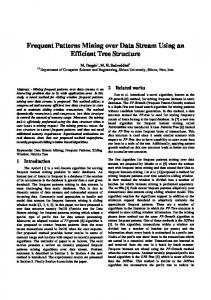
Figure 1. The FP-stream structures. Example 1 Consider the following stream of transactions: Batch first

second

third

Transactions t1 t2 t3 t4 t5 t6 t7 t8 t9

Contents {a, b, c, d} {a, d} {a, b} {a, b, c, e} {a, d, e} {c, e} {a, d} {a, c, d, e} {c, e}

Let the window size be 2 batches (indicating that only two batches of transactions are kept). Then, when the first batch of transactions in the stream flows in, FP-streaming calls the FP-growth algorithm (using preMinsup=2 instead of using minsup=3), which finds “frequent” patterns (with their frequencies) {a}:3, {b}:2, {d}:2, {a, b}:2, and {a, d}:2. These patterns are then stored in the FP-stream structure. Similarly, when the next batch flows in, FP-streaming again calls FPgrowth to find “frequent” patterns {a}:2, {c}:2, {e}:3, {a, e}:2, and {c, e}:2. These patterns are then stored in the FP-stream structure. See Figure 1; node e:0:3 indicates that itemset {e} has a frequency of 0 in the first batch and 3 in the second one. After FP-growth finds “frequent” patterns {a}:2, {c}:2, {d}:2, {e}:2, {a, d}:2, and {c, e}:2 for the third batch, the window slides from capturing the first & second batches of transactions to capturing the second & third batches. The FP-stream needs to be updated, and frequency values of each node need to be shifted so as to reflect the slid window. See Figure 1. (Note that nodes b with frequency 0:0 could be pruned.)

While the FP-streaming algorithm can handle data streams, but it does not handle constraints. Moreover, the algorithm uses preMinsup (which is ≤ minsup). This is just a heuristic. In other words, the completeness of frequency values for the frequent patterns returned by the algorithm depends on the value of preMinsup. If it is set too high (i.e., too close to minsup), some potentially frequent but currently infrequent itemsets may have been pruned too early and thereby losing their frequency values.

3. Integrating constrained mining with stream mining: an approximate algorithm In this section, we describe how we integrate constrained mining with stream mining in a tree-based framework. Let us start with a na¨ıve approach, which we call FP-streaming++. It first applies FP-streaming (an unconstrained mining algorithm) to find “frequent” patterns from streams, and then applies constraint checking as a postprocessing step to check if these “frequent” patterns satisfy the user constraint C. Recall from Section 2 that FPstreaming consists of two key steps: It first calls the FP-

growth algorithm with preMinsup to find “frequent” patterns, and then stores and maintains these “frequent” patterns in a tree structure called FP-stream. While simple, FP-streaming++ suffers from at least the following problems/weaknesses: 1. As constraint checking is a post-processing step (i.e., constraint C is not pushed inside the mining algorithm to effect pruning as early as possible), the number of patterns stored in the FP-stream is not proportional to the selectivity of C. This problem is worsened when C is a highly selective one (i.e., when only a tiny fraction of “frequent” patterns satisfy C). 2. For the same reason, the computation for mining is also not proportional to the selectivity of C. 3. As the use of preMinsup is just a heuristic, there is no guarantee that all and only those frequent patterns (with complete frequency information) can be found. An improved approach, which we call FP-streaming*, is to push the constraint C inside the FP-streaming algorithm. A deep look at the FP-streaming algorithm reveals that the number of “frequent” patterns stored in the FP-stream depends on the number of patterns generated by FP-growth. So, if we apply the post-processing step of checking C earlier (say, after obtaining “frequent” patterns from FPgrowth but before storing them in the FP-stream), we could reduce the size of the FP-stream. By so doing, the number of “frequent” patterns to be stored in the FP-stream is proportional to the selectivity of C. This solves Problem 1. How about the other two problems/weaknesses?

3.1. Finding from streams the patterns that satisfy succinct anti-monotone constraints Recall that a constraint can be succinct, and/or antimonotone, or neither. While FP-streaming* works well for the general case (i.e., any constraint C—regardless of whether it is succinct or not), we could do better if C is succinct. Specifically, we could push a succinct constraint C deeper inside the mining process (i.e., inside the FP-growth algorithm used in the first step of FP-streaming). In this section, we propose an approximate algorithm, called approxCFPS, for mining constrained frequent patterns (i.e., frequent patterns that satisfy succinct constraints) from streams. Our algorithm consists of the following main operations: (i) constraint checking of transactions in the current batch, (ii) construction of an FP-tree for this current batch, (iii) recursive growth of valid “frequent” patterns, and (iv) storing of these patterns in an FP-stream structure. Note that a succinct constraint can also be antimonotone. We call those succinct anti-monotone constraints as SAM constraints and those succinct non-antimonotone constraints as SUC constraints. Let us first show how our approxCFPS algorithm handles a SAM constraint CSAM . The algorithm exploits two nice proper-

ties of CSAM : (i) anti-monotonicity (i.e., if a pattern violates CSAM , then all its supersets also violate CSAM ) and (ii) succinctness (i.e., one can easily enumerate all and only those patterns that are guaranteed to satisfy CSAM ). Hence, any pattern ν satisfying CSAM must consist of only items that individually satisfy CSAM . In other words, ν ⊆ ItemM (i.e., the set of items that individually satisfy CSAM ). Due to succinctness, items in ItemM can be efficiently enumerated. Our approxCFPS algorithm discovers frequent patterns satisfying CSAM as follows. We first apply constraint checking on all domain items in order to find ItemM . We then extract from the incoming batch of streaming transactions those items that are in ItemM , and capture them in an FP-tree. Items that are not in ItemM can be discarded because any patterns contain any non-ItemM item do not satisfy CSAM . Once these ItemM items are found, all we need to do is to recursively apply the usual FP-tree based mining process to each projected database of “frequent” patterns (i.e., apply to each α-projected database—which is a collection of transactions having α as its prefix—where α ⊆ ItemM ). Like FP-streaming, we also use preMinsup (instead of minsup) during the mining process. At the end, we find all valid “frequent” patterns and store them in the FP-stream structure. To gain a better understanding of how our approxCFPS algorithm handles CSAM , let us consider the following example. Example 2 Consider the first batch of transactions shown in Example 1. Assume that the prices of items a, b, c, d are 60, 10, 30, 40 respectively. Let constraint CSAM be the SAM constraint Q1 ≡ min(S.P rice) ≥ 20, minsup be 3, and preMinsup be 2. Our proposed approxCFPS algorithm discovers valid “frequent” itemsets as follows. It first enumerates from the domain items those valid items a, c, d (i.e., items with individual P rice ≥ 20). Among them, item c is infrequent (with frequency < preMinsup) and is thus removed. Then, approxCFPS builds an FP-tree. Afterwards, the usual FP-tree based mining process (with only frequency check) is applied recursively to subsequent projected databases. As a result, valid “frequent” itemsets {a}:3, {d}:2, and {a, d}:2 are found. These itemsets are then stored in the FP-stream structure in the same fashion as in FP-streaming. Note that approxCFPS (which computes only three valid “frequent” itemsets and stores them in the FP-stream) requires less computation and storage space than FP-streaming++ (which computes five “frequent” itemsets and stores them in the FP-stream, but only three of them are valid) and FP-streaming* (which also computes five “frequent” itemsets, but stores only the three valid ones in the FP-stream).

3.2. Finding from streams the patterns that satisfy succinct non-anti-monotone constraints Next, let us turn our attention to how our approxCFPS algorithm handles a SUC constraint CSUC . Note that for SUC constraints, they satisfy the “succinctness” property so that one can easily enumerate all and only those patterns that are guaranteed to satisfy CSUC . However, SUC constraint do not satisfy the “anti-monotonicity” property. In

other words, if a pattern violate CSUC , there is no guarantee that all or any of its supersets would violate CSUC . Hence, not all valid patterns are composed of only mandatory items (as for SAM constraints). Instead, any pattern ν satisfying CSUC is composed of mandatory items (i.e., items satisfying CSUC ) and possibly some optional items (i.e., items not satisfying CSUC ). In other words, a valid pattern ν is usually of the form α ∪ β, where (i) α ⊆ ItemM (the set of mandatory items) such that α = ∅, and (ii) β ⊆ ItemO (the set of optional items). Due to succinctness, items in ItemM and ItemO can be efficiently enumerated. Hence, we cannot apply the same procedure as we did for CSAM . Some modification is needed; otherwise, we may miss some valid frequent patterns. Specifically, our approxCFPS discovers frequent patterns satisfying CSUC as follows. We first apply constraint checking in order to divide the domain items into two sets—the set ItemM consisting of all mandatory items and the set ItemO consisting of all optional items. We then extract from the incoming batch of streaming transactions the items that belong to these two sets. These items are captured in an FP-tree in such a way that mandatory items appear below optional items (i.e., mandatory items are closer to the leaves, and optional items are closer to the root). With this item-ordering scheme, all we need to do is to recursively apply the usual FP-tree based mining process to each projected database of only those valid “frequent” patterns (i.e., apply to each α-projected database—which is a collection of transactions having α as its prefix—where α ⊆ ItemM ), because all patterns satisfying CSUC must be “extensions” of items from ItemM (i.e., all valid patterns must be grown from ItemM items). At the end of the mining process, we find all valid “frequent” patterns and store them in the FP-stream structure. See the following example. Example 3 Consider the first batch of transactions shown in Example 1. Assume that the quantities of items a, b, c, d be 100, 500, 250, 300. Let constraint CSU C be the SUC constraint Q3 ≡ max(S.Qty) ≥ 300, minsup be 3, and preMinsup be 2. Our approxCFPS algorithm discovers valid “frequent” itemsets as follows. It first partitions the domain items into two sets (i.e., enumerates members of each set): (i) the mandatory set containing items b, d (i.e., times with individual Qty ≥ 300), and (ii) the optional set containing items a, c (i.e., times with individual Qty < 300). Then, approxCFPS builds an initial FP-tree (i.e., the FP-tree capturing this batch of transactions), in which all mandatory items appear below optional items. Note that for CSU C , this “boundary” between mandatory and optional items only exists in this initial FP-tree, but not in any FP-trees built for subsequent projected databases. Once a projected database is formed for each valid “frequent” singleton itemset (e.g., {b}, {d}), there is no distinction between mandatory and optional items. In other words, once a valid itemset ν contains a mandatory item, any other items in ν can be chosen from the mandatory or the optional sets. This explains why once approxCFPS forms the {b}- and {d}-projected databases, the usual FPtree based mining process (with only frequency check) can be applied recursively to subsequent projected databases. As a result, valid “frequent” patterns {b}:2 and {d}:2 (singleton patterns), as well as {a, b}:2 (from the {b}-projected database) and {a, d}:2 (from the {d}-projected database), are found. These patterns are then stored in the FP-stream structure in the same fashion as in FP-streaming.

To summarize, our proposed approxCFPS algorithm exploits the properties of succinct constraints (CSAM or CSUC ), and pushes these constraints deeper inside the mining process (i.e., inside the FP-growth algorithm used in FP-streaming). As a result, pruning for constraint satisfaction is done once-and-for-all at the initial step when approxCFPS enumerates all the individually valid items (i.e., ItemM items). At recursive steps/projected databases, all the valid “frequent” patterns can be grown from the projected databases of these ItemM items, and no constraint checking is required. This solves our Problem 2; hence, the number of patterns stored in the FP-stream structure as well as the computation for mining is proportional to the selectivity of constraints.

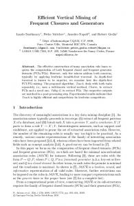
4. Integrating constrained mining with stream mining: an exact algorithm In this section, we show how we deal with Problem 3. Like FP-streaming, our approxCFPS algorithm also uses preMinsup during the mining process (FP-growth). The reason is that, when dealing with data streams, a currently infrequent pattern may become frequent in the future. So, we better not prune these patterns too early; otherwise, we lose frequency information about these patterns. However, the use of preMinsup is just a heuristic. Its success strongly depends on the value of preMinsup. If it is too high (e.g., too close to minsup), we may lose frequency information of some patterns. To another extreme, if it is too low, lots of redundant patterns (e.g. those patterns with frequency lower than minsup but not lower than preMinsup) may be generated and stored in the FP-stream structure. In this section, we propose an exact algorithm, called exactCFPS, for mining from streams those frequent patterns that satisfy succinct constraints. Here, we combine the FP-tree with the FP-stream structure. Our proposed algorithm consists of the following main operations: (i) constraint checking of transactions in the current batch, (ii) construction of a modified FP-tree, and (iii) recursive growth of valid truly frequent patterns from the modified FP-tree. There is no need for preMinsup or the FP-stream structure. Specifically, the exactCFPS algorithm discovers constrained frequent patterns from streams as follows. When a batch of transactions flows in, we first exploit constraints (CSAM or CSUC ) and push constraints deep into the mining process (i.e., deep inside FP-growth) in the same fashion that we did in approxCFPS. In other words, if it is a SAM constraint, we apply constraint checking on all items in the transactions to find those belong to ItemM ; if it is a SUC constraint, we apply constraint checking on all items in the transactions to divide the items into two sets (one for ItemM and another for ItemO ). Then, we insert all those transactions into an modified FP-tree where (i) each tree path represents a transaction and (ii) each tree node contains a list of

a:3:2 c:1:1

d:1:1

c:0:1 e:0:1

d:1:0 e:0:1 e:0:1

a:2:2 c:1:1

d:1:1

c:1:1 e:1:1

d:0:1 e:1:0 e:1:0 e:0:1

At time T (The modified FP-tree capturing 1st & 2nd batches)

At time T’ (The modified FP-tree capturing 2nd & 3rd batches)

Figure 2. Modified FP-trees for exactCFPS. frequency value (instead of just one frequency value). Also, we keep all (frequent and infrequent) items: all ItemM items for CSAM , all ItemM and ItemO items for CSUC . This is because a currently infrequent item may become frequent in the future. Then, when the next batch of transactions flows in, we shift the frequency values in the list at each node by removing the frequency value of the oldest batch of transactions and appending the frequency value of the newest batch. At any point T in time, this modified FP-tree captures the most important portion (usually the recent portion w.r.t. T ) of the streams so that truly frequent patterns (using the regular minsup) can be mined from the modified FPtree. Since constraint checking has been done at the initial step and no further constraint checking is needed at recursive steps/projected databases (due to succinctness), all we need to do is to recursively apply the usual FP-tree based mining process to each projected database of valid frequent patterns. See the following examples. Example 4 Consider the same batch of streaming data, auxiliary item information, and CSAM as in Example 2. Our proposed exactCFPS algorithm discovers valid truly frequent itemsets as follows. It first enumerates from the domain items those valid items a, c, d. Then, exactCFPS inserts transactions (with invalid items removed from batches of transactions) into a modified FP-tree. When users want to find constrained frequent patterns, the usual FPtree based mining process (with only frequency check) can then be applied recursively to subsequent projected databases of this modified FP-tree. As a result, a valid truly frequent itemset {a}:3 can be found from this first batch of transactions in the data stream. Example 5 Consider the streaming data in Example 1, the same auxiliary item information and CSAM as in Example 4. Then, during the insertion of transactions from the data stream, only nb = 2 frequency values are kept for each node in the modified FP-tree because the window size nb is 2. See the content of the modified FP-trees in Figure 2. At time T when the first two batches are read, the usual FP-tree based mining process (with only frequency check) can be applied recursively to subsequent projected databases to find valid truly frequent patterns (using minsup) from the modified FP-tree. This is because the tree captures the two most recent batches of transactions w.r.t. T . Then, at time T when the third batch is read, the modified FP-tree needs to be updated to capture the two most recent batches w.r.t. T (the second and third batches) and discard the oldest batch in the window (e.g., the first batch). Specifically, when the window slides, the list of frequency values of each tree node is also shifted. See Figure 2.

So far, we have proposed and discussed several algorithms. Let us compare them in Table 1. These algorithms

Table 1. Our proposed algorithms vs. the most relevant algorithms. Algorithms

CAP [22], DCF [18] √ √

Constrained mining: Find constrained frequent patterns Mining is proportional to constraint selectivity Tree-based mining: Use an FP-tree Mine only valid, truly frequent patterns from the FP-tree Mine only valid “frequent” patterns from the FP-tree Mine all “frequent” patterns from the FP-tree Stream mining Do not need the FP-stream structure Use an FP-stream structure: The FP-stream stores only valid “frequent” patterns The FP-stream stores all “frequent” patterns

e:6

e:6

f:5

f:5

f:5 g:2 h:2

g:2 h:2

g:2 h:2 Modified FP-tree

g:2

h:2

g:2 h:2 FP-stream

Figure 3. Modified FP-tree vs. the FP-stream. tried to integrate constrained mining with stream mining in a tree-based framework. Among them, exactCFPS may appear to require more space than approxCFPS because the modified FP-tree for exactCFPS can be bigger than the original FP-tree for approxCFPS. However, it is not always the case; see Figure 3. It is also important to note an advantage of exactCFPS: It does not require keeping an extra tree structure (i.e., no FP-stream) and does not require using preMinsup. This solves Problem 3. Among the algorithms that require the FP-stream structure, FP-streaming* and approxCFPS require less storage space than FP-streaming++. This is because the former two store only valid patterns (i.e., patterns satisfying constraints), whereas FP-streaming++ stores all patterns (valid as well as invalid ones). In terms of mining, both FP-streaming++ and FPstreaming* do not push constraints inside the mining process; so, they both find valid as well as invalid patterns. In contrast, both approxCFPS and exactCFPS push constraints deep inside the mining process; so, they both find only valid patterns. Consequently, the computation is proportional to the selectivity of constraints. Moreover, although we presented our exactCFPS as an algorithm to find constrained frequent patterns from data streams, the algorithm can be easily be adapted for mining other patterns such as maximal or closed patterns.

5. Experimental results The experimental results cited below are based on streaming data generated by the program developed at IBM Almaden Research Center [2]. The data contain 1M records

FP-streaming [12]

FPstreaming++ √

FPstreaming* √

√

√

√

√ √

√ √

√ √

√

√

√

√

√ √

approxCFPS √ √ √ √ √ √ √

exactCFPS √ √ √ √

√ √

with an average transaction length of 10 items, and a domain of 1,000 items. Unless otherwise specified, we used minsup = 0.01% and preMinsup = 0.0025%. We set each batch be of size 50,000 transactions and the window size be of two batches. All experiments were run in a timesharing environment in a 700 MHz machine. The reported figures are based on the average of multiple runs. Runtime includes CPU and I/Os; it includes the time for FP-tree construction, frequent-pattern mining, and FP-stream construction steps (if appropriate). In the experiments, we compared the following algorithms that were implemented in C: (i) the na¨ıve approach (FP-streaming++), (ii) the improved approach (FP-streaming*), (iii) our approximate algorithm (approxCFPS), and (iv) our exact algorithm (exactCFPS). In the first set of experiments, we evaluated the effectiveness of constrained mining. We compared the runtimes of various algorithms. The y-axis of Figure 4 shows the runtime, and the x-axis shows the selectivity of the succinct constraint. A constraint with pct% selectivity means pct% of items is selected. The higher the pct value, the more is the number of selected items. It is observed from Figure 4(a) that as the selectivity of the SAM constraint CSAM decreased (i.e., fewer items are selected), the runtime remained unchanged for FPstreaming++. It is because FP-streaming++ ignores CSAM at the early stage of the mining process, mines from the FPtree that captures each incoming batch of streaming transactions to find all (valid and invalid) “frequent” patterns, stores them in the FP-stream (regardless of selectivity), and conducts constraint checking as a post-processing step. For FP-streaming*, as the selectivity of CSAM decreased, the runtime decreased slightly. It is because FP-streaming* also ignores CSAM at the early stage of the mining process and finds all “frequent” patterns (regardless of selectivity), but it stores only valid ones in the FP-stream. On the other hands, the runtimes for approxCFPS and exactCFPS decreased gradually as the selectivity decreased. This shows that the runtimes required by approxCFPS and exactCFPS depend on selectivity. Specifically, approxCFPS pushes

Handling the SAM constraint

Handling the SUC constraint FP-streaming++ FP-streaming* approxCFPS exactCFPS

300

250 Runtime (in seconds)

250 Runtime (in seconds)

FP-streaming++ FP-streaming* approxCFPS exactCFPS

300

200

150

200

150

100

100

50

50

0

0 10

20

30 40 50 60 70 Selectivity (i.e., percentage of items selected)

80

90

10

20

(a) The SAM Constraint


80

90

(b) The SUC Constraint

Figure 4. Runtime with succinct constraints. Handling the SAM constraint

Handling the SUC constraint 400

FP-streaming++ FP-streaming*, approxCFPS

400

FP-streaming++ FP-streaming*, approxCFPS

380

Size of the FP-stream (in MB)

Size of the FP-stream (in MB)

390

360

340

380

370

360

350

320 340

300

330 10

20


80

90

(a) The SAM Constraint

10

20


80

90

(b) The SUC Constraint

Figure 5. Memory space (Size of the FP-stream for succinct constraints). CSAM inside the mining process and finds only valid “frequent” patterns (i.e., ignores invalid ones) from the FPtree that captures each incoming batch of streaming transactions, stores them in the FP-stream. For exactCFPS, it also pushes CSAM inside the mining process, but it mines valid truly frequent patterns from a modified FP-tree that captures the nb recent batches of streaming transactions. No FP-stream structure is needed. So, for both algorithms, the number of valid patterns depends on the selectivity of CSAM . The computation for mining is proportional to the selectivity of the SAM constraint. Figure 4(b) shows the results for the SUC constraints. Again, the computation for mining using the approxCFPS and the exactCFPS algorithms is proportional to the selectivity of the SUC constraint. It is important to note that, for succinct constraints (CSAM or CSUC ), constraint checking is performed early at the initial step instead of as a postprocessing step. In the second set of experiments, we compared the size of the FP-stream structure (i.e., space required by the FP-

stream). The y-axis of Figure 5 shows the sizes of FPstream, and the x-axis shows the selectivity of the succinct constraint. Again, Figure 5(a) shows the results for CSAM while Figure 5(b) shows the results for CSUC . It is observed that as the selectivity of the constraints decreased (i.e., fewer items were selected), the size of the FP-stream remained unchanged for FP-streaming++. This is because FP-streaming++ finds all “frequent” patterns and stores them in the FP-stream (regardless of constraint selectivity). On the other hands, the sizes of the FP-stream for both FP-streaming* and approxCFPS decreased as the selectivity decreased because only valid “frequent” patterns were stored in the FP-stream structures. The experimental results show that the sizes of the FP-stream required by these two algorithms depends on constraint selectivity and were the same (due to the same collection of valid “frequent” patterns). The number of patterns stored in the FPstream in proportional to the selectivity of constraints. In the third set of experiments, we compared the tree size. We observed that as the selectivity of the constraints

decreased (i.e., fewer items were selected), the sizes of the FP-trees remained unchanged for both FP-streaming++ and FP-streaming* because they keep all “frequent” items in the trees. On the other hands, the size of the FP-tree for approxCFPS and that of the modified exactCFPS decreased as the selectivity decreased because they keep only valid items in the trees. Regarding the size of the modified FP-tree for exactCFP, it was just 1.39× the size of the FP-tree and the FP-stream used in approxCFPS when selectivity was 10%; this ratio decreased to 1.09× when selectivity was 90%. In addition to the above three sets of experiments, we have also evaluated the effects of various minsup on runtime. As expected, when the minsup increased, the runtimes of all algorithms decreased. Note that, when minsup increased, the size of FP-trees decreased for all algorithms. As a result, smaller FP-tree was needed to be traversed during the mining process, and thereby reducing the runtimes. Moreover, fewer patterns were considered frequent. This implied fewer patterns were needed to be stored in the FPstream (except for the exactCFPS algorithm, which do not use the FP-stream at all). Furthermore, we run scalability test. The results showed linear scalability (w.r.t. the number of transactions in a batch as well as the number of batches) for these algorithms. To summarize, the above results show the importance and the benefits of using our developed algorithms for efficient mining of the frequent patterns that satisfy the user constraints from the flood of data (i.e., efficient constrained frequent-pattern mining from streams).

6. Conclusions A key contribution of this paper is to develop efficient approximate and exact algorithms—called approxCFPS and exactCFPS, respectively—for mining constrained frequent patterns from streams. These algorithms are a non-trivial integration of constrained mining, tree-based mining, and stream mining. Consequently, they (i) enable human users to impose a certain focus on the mining process, (ii) capture the important portion of streaming data, and (iii) find constrained frequent patterns with complete frequency information. Among the two algorithms, approxCFPS finds constrained approximately “frequent” patterns (i.e., all frequent patterns together with some sub-frequent patterns) and stores them in an FP-stream structure, whereas exactCFPS modifies the FP-tree for mining and combines it with the FP-stream into a data structure for exact mining for constrained frequent patterns. By pushing constraints deep inside the mining process, the amount of mining computation and item storage in the tree is proportional to the selectivity of constraints.

Acknowledgement. This project is partially sponsored by Natural Sciences and Engineering Research Council of Canada (NSERC) and The University of Manitoba in the form of research grants.

References [1] R. Agrawal, T. Imielinski, and A. Swami. Mining association rules between sets of items in large databases. In Proc. SIGMOD 1993, pp. 207–216. [2] R. Agrawal and R. Srikant. Fast algorithms for mining association rules. In Proc. VLDB 1994, pp. 487–499. [3] R.J. Bayardo. Efficiently mining long patterns from databases. In Proc. SIGMOD 1998, pp. 85–93. [4] R.J. Bayardo, R. Agrawal, and D. Gunopulos. Constraint-based rule mining in large, dense databases. In Proc. ICDE 1999, pp. 188–197. [5] J.-F. Boulicaut and B. Jeudy. Mining free itemsets under constraints. In Proc. IDEAS 2001, pp. 322-329. [6] S. Brin, R. Motwani, and C. Silverstein. Beyond market baskets: generalizing association rules to correlations. In Proc. SIGMOD 1997, pp. 265–276. [7] D.W. Cheung et al. Maintenance of discovered association rules in large databases: an incremental updating technique. In Proc. ICDE 1996, pp. 106–114. [8] W. Cheung and O.R. Za¨ıane. Incremental mining of frequent patterns with candidate generation or support constraint. In Proc. IDEAS 2003, pp. 111–116. [9] Y. Chi et al. Moment: maintaining closed frequent itemsets over a stream sliding window. In Proc. ICDM 2004, pp. 59–66. [10] M.M. Gaber, A.B. Zaslavsky, and S. Krishnaswamy. Mining data streams: a review. SIGMOD Record, 34(2), Jun. 2005, pp. 18–26. [11] M.N. Garofalakis, R. Rastogi, and K. Shim. SPIRIT: sequential pattern mining with regular expression constraints. In Proc. VLDB 1999, pp. 223–234. [12] C. Giannella et al. Mining frequent patterns in data streams at multiple time granularities. In Data Mining: Next Generation Challenges and Future Directions, AAAI/MIT Press, 2004, ch. 6. [13] G. Grahne, L.V.S. Lakshmanan, and X. Wang. Efficient mining of constrained correlated sets. In Proc. ICDE 2000, pp. 512–521. [14] J. Han, J. Pei, and Y. Yin. Mining frequent patterns without candidate generation. In Proc. SIGMOD 2000, pp. 1–12. [15] R.J. Hilderman et al. Mining market basket data using share measures and characterized itemsets. In Proc. PAKDD 1998, pp. 159– 170. [16] N. Jiang and L. Gruenwald. Research issues in data stream association rule mining. SIGMOD Record, 35(1), Mar. 2006, pp. 14–19. [17] R.M. Karp, S. Shenker, and C.H. Papadimitriou. A simple algorithm for finding frequent elements in streams and bags. ACM TODS, 28(1), Mar. 2003, pp. 51–55. [18] L.V.S. Lakshmanan, C.K.-S. Leung, and R. Ng. Efficient dynamic mining of constrained frequent sets. ACM TODS, 28(4), Dec. 2003, pp. 337–389. [19] C.K.-S. Leung, Q.I. Khan, and T. Hoque. CanTree: a tree structure for efficient incremental mining of frequent patterns. In Proc. ICDM 2005, pp. 274–281. [20] C.K.-S. Leung, R.T. Ng, and H. Mannila. OSSM: a segmentation approach to optimize frequency counting. In Proc. ICDE 2002, pp. 583–592. [21] R.J. Miller and Y. Yang. Association rules over interval data. In Proc. SIGMOD 1997, pp. 452–461. [22] R.T. Ng et al. Exploratory mining and pruning optimizations of constrained associations rules. In Proc. SIGMOD 1998, pp. 13–24. [23] J.S. Park, M.-S. Chen, and P.S. Yu. Using a hash-based method with transaction trimming for mining association rules. IEEE TKDE, 9(5), Sep./Oct. 1997, pp. 813–825. [24] R. Srikant, Q. Vu, and R. Agrawal. Mining association rules with item constraints. In Proc. KDD 1997, pp. 67–73. [25] J.X. Yu et al. False positive or false negative: mining frequent itemsets from high speed transactional data streams. In Proc. VLDB 2004, pp. 204–215.