called recursive transition networks with string output (RTNSO). RTNSO-based ... sis and the representation of the elementary sentence struc- tures of a natural ...
Efficient parsing using recursive transition networks with output Javier M. Sastre∗† , Mikel L. Forcada† ∗
†
Institut Gaspard-Monge, Universit´e Paris Est, F-77454 Marne-la-Vall´ee Cedex 2, France
Grup Transducens, Departament de Llenguatges i Sistemes Inform`atics, Universitat d’Alacant, E-03071 Alacant, Spain. Abstract
We describe here two efficient parsing algorithms for natural language texts based on an extension of recursive transition networks (RTN) called recursive transition networks with string output (RTNSO). RTNSO-based grammars may be semiautomatically built from samples of a manually built syntactic lexicon. Efficient parsing algorithms are needed to minimize the temporal cost associated to the size of the resulting networks. We focus our algorithms on the RTNSO formalism due to its simplicity which facilitates the manual construction and maintenance of RTNSO-based linguistic data as well as their exploitation.
1. Introduction This paper describes two efficient parsing algorithms for natural language texts which use recursive transition networks (Woods, 1970) (RTNs) generated from a large and manually built syntactic lexicon such as the one defined in (Gross, 1975). Both algorithms are easily defined based on the formal definition of RTN with string output1 (RTNSOs) given in section 2., which corresponds to a special type of pushdown letter transducer (a pushdown automaton with output), and the formal definition of the set of outputs (such as parses or translations) associated to an input string given in section 3. A first algorithm for the efficient computation of that set is given in section 4., paying special attention to null closure due to its crucial role in the algorithm. An explanation of how to modify the preceding algorithm in order to obtain a more complex but also more efficient Earley-like algorithm is given in section 5. Comparative results are given in section 6. Concluding remarks close the paper. 1.1. Parsing with RTNs and lexicon-grammar Lexicon-grammar is a systematic method for the analysis and the representation of the elementary sentence structures of a natural language (Gross, 1996) which has produced, over the last 30 years, a large and fine-grain linguistic resource2 describing syntactic and semantic properties of French simple sentences (among other languages) for 13375 simple verbs, 10325 predicative nouns (e.g.: pride as in to be proud of) and 39297 idiomatic expressions playing the role of predicative element (e.g.: to wear the pants). There exists a technique to semiautomatically build a RTNbased grammar from samples of the lexicon-grammar for automatic parsing (Roche, 1993). Although the RTN formalism is not the most expressive, its simplicity has permitted its practical application to the analysis of specialized domain corpora (Nakamura, 2004) with RTN-based computer tools (INTEX (Silberztein, 1993), Unitex (Paumier, 2006), Outilex (Blanc et al., 2006)). However, the 1
For instance, the result of parsing as a tagged input. Partially available through the HOOP interface (Sastre, 2006) at http://hoop.univ-mlv.fr 2
temporal cost of applying a large RTN to a large corpus may be too high for certain applications. We expect to reduce it by employing efficient parsing algorithms.
2. Recursive transition networks with string output A non-deterministic RTNSO R = (Q, Σ, Γ, δ, QI , F ) is made of a finite set of states Q = {q1 , q2 , . . . , q|Q| } (which will also be used as the alphabet for the pushdown stack), a finite input alphabet Σ = {σ1 , σ2 , . . . , σ|Σ| }, a finite output alphabet Γ = {γ1 , γ2 , . . . , γ|Γ| }, QI ⊆ Q the set of initial states, F ⊆ Q the set of acceptance states, and a transition function δ : Q×((Σ∪{ε})×(Γ∪{ε})) → P(Q×(Q∪{λ})) (1) where P(·) represents the set of all subsets of a given set and λ ∈ Q∗ is an empty sequence of states. As to the possible types of transitions: • Transitions of the form δ(q, (σ, γ)) with σ ∈ Σ and γ ∈ Γ read one input symbol and write an output symbol; those of the form δ(q, (σ, ε)) read a symbol but do not write anything, those of the form δ(q, (ε, γ)) do not read an input symbol but write an output symbol, and those of the form δ(q, (ε, ε)) neither read nor write symbols. • Only transitions of the form δ(q, (ε, ε)) can contain elements of Q × Q in their result set; that is, only transitions without input and output can push a state onto the stack. These transitions represent a call: in addition to performing a transition to a new state, they push a return state onto the stack which will be popped later: (qc , qr ) ∈ δ(qs , (ε, ε)) represents a subroutine jump to state qc which pushes the return state qr onto the stack. The rest of the transitions can only return elements of Q × {λ}, that is, they do not push anything onto the stack. • It has to be noted that δ does not define any transitions which pop states from the stack. This is because states can be automatically popped from a nonempty stack
everytime the RTNSO reaches an acceptance state in F ; the popped state is reached without consuming any input or writing any output. The definition of popping transitions is implicit in the definition of R. • As a general rule, loops consuming no input but generating output or making calls are not allowed: infinite length parses of natural-language input sequences make no sense and complicate the correspondent parsing algorithms which should avoid falling into infinite loops.
In this section we will formally derive the computation of the set of output translations associated to an input string following (Garrido-Alenda et al., 2002). During the application of a RTNSO, a triplet (q, z, π) ∈ Q × Γ∗ × Q∗ represents the fact that a partial output (PO) z has been generated up to the point of reaching state q with a stack π. We call V ∈ P(Q × Γ∗ × Q∗ ) a set of POs (SPO); we define ∆ as the PO transition function over a SPO for an input symbol as (2)
∆(V, σ) = {(q 0 , zg, π) : (q 0 , λ) ∈ δ(q, (σ, g)) ∧ (q, z, π) ∈ V }, (3) where q, q 0 , qc , qr ∈ Q, z ∈ Γ∗ is an output string, π ∈ Q∗ a stack, σ ∈ Σ an input symbol, and g ∈ Γ ∪ {ε} an output symbol or an empty output. We define the ε-closure Cε (V ) of a SPO V , Cε : P(Q × Γ∗ × Q∗ ) → P(Q × Γ∗ × Q∗ ),
(4)
as the smallest SPO containing V and every PO directly or indirectly derivable from V through ε-transitions, that is, through zero, one or more transitions without consuming any input symbol. Informally, elements are added to the ε-closure through three different kinds of ε-moves until no more elements are added: • Output without input: adding (q 0 , zg, π) for each (q, z, π) in the closure and for each q 0 and g such that (q 0 , λ) ∈ δ(q, (ε, g)); • Call or push: adding (qc , z, πqr ) for each (q, z, π) in the closure and for each qc and qr such that (qc , qr ) ∈ δ(q, (ε, ε)); • Return or pop: adding (qr , z, π) for each (q, z, πqr ) in the closure such that q ∈ F ; An efficient way to compute the ε-closure is described in section 4. We recursively define ∆∗ : P(Q × Γ∗ × Q∗ ) × Σ∗ → P(Q × Γ∗ × Q∗ ), (5) the extension of ∆ to strings in Σ∗ , as follows: ∆∗ (V, ε) = Cε (V ) ∆∗ (V, zσ) = Cε (∆(∆∗ (V, z), σ))
T (σ1 . . . σl ) = {z ∈ Γ∗ : (q, z, λ) ∈ ∆∗ (QI × {ε} × {λ}, σ1 . . . σl ) ∧ q ∈ F }. (8)
4. Processing an input string
3. Language of translations of a string
∆ : P(Q × Γ∗ × Q∗ ) × Σ → P(Q × Γ∗ × Q∗ )
Finally, we define T (σ1 . . . σl ) the language of translations of input string σ1 . . . σl as the set of output strings of the final part of the SPO (having only final states and no pending return-from-call states) reachable from the initial SPO (having every initial state coupled with an empty output string and an empty return stack) through zero, one or more transitions and consuming the whole input string:
(6) (7)
Based on the formal definition given in the previous section, we propose a breadth-first algorithm decomposed into algorithms 1 (translate string), 2 (translate symbol), and 3 (closure) to process an input string for a given (nondeterministic) RTNSO and to generate the set of corresponding output strings based on the equations above. The algorithm keeps for each prefix of the input string a SPO V , whose elements are triplets of the form (q, z, π) where q ∈ Q is a state, z ∈ Γ∗ is an output string and π ∈ Q∗ is a last-in-first-out stack holding states in Q (λ will be used to represent the empty stack), as described in the previous section. In the algorithms, the RTNSO R = (Q, Σ, Γ, δ, QI , F ) is treated as a global variable. Based on van Noord’s per subset algorithm (van Noord, 2000), algorithm 3 is an efficient algorithm for the computation of the ε-closure of a given SPO V . To start it copies V into E; then it uses V to store the result of the computation and E to keep a trace of the partial outputs that have not been processed yet. V is iteratively incremented with the new reachable states from an arbitrary partial output of E by one ε-transition. Each time a partial output of E is retrieved ((q, z, π) ← next(E)) to be processed, it is also removed from E. Each time a new partial output is added to V (if (add(V, (q, z, π))), it is also added to E (insert(E, (q, z, π)) for further processing. The difference between add() and insert() is that the former performs a duplicity test before adding the PO to V and returns the boolean result of this test, and the latter adds the PO blindly to E and returns nothing. Algorithm 1 translate string(σ1 . . . σl ) . T , eq. (8) Input: σ1 σ2 . . . σl , an input string of length l Output: T , the set of translations 1: V ← closure(QI × {ε} × {λ}) . initial SPO V0 2: i ← 0 3: while V 6= ∅ ∧ i < l do . Vi+1 = Cε (∆(Vi , σi+1 )) 4: V ← closure(translate symbol(V, σi+1 )) 5: i←i+1 6: end while 7: T ← ∅ 8: if i = l then 9: for each (q, z, λ) ∈ V : q ∈ F do 10: T ← T ∪ {z} 11: end for 12: end if As can be seen, the algorithm is quite simple and does not require a complex data structure. At each iteration it
Algorithm 2 translate symbol(V, σ) . ∆(V, σ), eq. (3) Input: V , the SPO σ, the symbol Output: W , the SPO after processing σ 1: W ← ∅ 2: for each (q, z, π) ∈ V do 3: for each (q 0 , g) : (q 0 , λ) ∈ δ(q, (σ, g)) do 4: W ← W ∪ {(q 0 , zg, π)} 5: end for 6: end for Algorithm 3 closure(V ) . Cε (V ) Input: V , the SPO whose ε-closure is to be computed Output: V after computing its ε-closure 1: E ← V . unprocessed PO queue 2: while E 6= ∅ do 3: (q, z, π) ← next(E) 4: for each (q 0 , g) : (q 0 , λ) ∈ δ(q, (ε, g)) do . ε5: if add(V, (q 0 , zg, π)) then . transitions 6: insert(E, (q 0 , zg, π)) 7: end if 8: end for 9: for each (qc , qr ) ∈ δ(q, (ε, ε)) do 10: if add(V, (qc , z, πqr )) then . push11: insert(E, (qc , z, πqr )) . transitions 12: end if 13: end for 14: if π = π 0 qr ∧ q ∈ F ∧ add(V, (qc , z, πqr )) then 15: insert(E, (qr , z, π 0 )) . pop-transition 16: end if 17: end while computes the SPO that can be derived from the precedent one by recognizing the next input symbol, so it suffices to store two SPOs at a time. It firstly fills in the next SPO with the POs directly reachable through one transition consuming the next input symbol, then it completes the SPO with the following reachable POs through one or more εtransitions, call and return transitions included. Two important limitations of the algorithm are: (a) the impossibility of parsing with RTNs representing left-recursive grammars since the computation of the ε-closure would try to generate a PO with an infinite stack of return states, and (b) the fact that for a SPO Vi having two POs with different stacks and/or outputs from where a call to a same state qc is performed, the computation of every PO derived from the call to qc is performed twice although it could be factored (for instance, for the RTNSO of Fig. 1 call to state q0 P is computed 2n+1 times for a string an bn when it could be computed n + 1 times by factoring out common calls). In the next section we show how to modify this algorithm to avoid both limitations.
5.
Earley-like RTNSO processing
Finite-state automata can give a compact representation of a set of sequences by factoring out common prefixes and suffixes. RTNs can also factor infixes by defining only a subautomaton for each repeated set of infixes and by using transitions calling the initial state of the corresponding subautomaton each time any infix in the set is to be recognized.
a : {
q1
q0
q2
b : }
ε :x
q0 a : [
q3
q0
q5 q4
b : ]
Figure 1: Example of RTNSO. Labels of the form x : y represent an input : output pair (e.g.: a : { for transition (δ(q0 , a, {) = (q1 , λ)). Dashed transitions represent a call to the state specified by the label (e.g.: transition (δ(q1 , ε, ε) = (q2 , q0 )). However, it is up to the parsing algorithm to detect that the same calling transition is made multiple times at an input point so the called subautomaton is processed only once. Based on Earley’s context-free grammar parsing algorithm (Earley, 1970)3, we show here a modified and more efficient version of the algorithm in section 4. which is able to process left-recursive RTNSOs, and which factores out the computation of infix calls by parallel analyses, as for the RTNSO of Fig. 1. We exchange the use of a return state stack for a more complex representation of POs, which mainly involves a modification of the ε-closure algorithm: when a call transition to a state qc is found, a paused PO until the completion of the call is generated as well as a new PO starting the called subanalysis from qc and the current input point, if not already started. Each time a subanalysis is completed, a resumed PO is generated for every concatenation of the paused POs depending on it and the substring generated by the subanalysis. 5.1. Language of translations through Earley-like processing POs are represented as 5-tuples (q, z, qc , qh , i) ∈ (Q × Γ∗ × (Q ∪ λ) × Q × N), where q is the current state, qh the state that initiated this subanalysis, i the input position where this subanalysis began (i representing the point between σi and σi+1 , so 0 is the point before the first input symbol), z the output generated from state qh and input position i up to state q and the current input position, and qc the start state of the subanalysis which this PO depends on (λ if no subanalysis completion is required, that is, for POs which are not paused but active). We extend the PO transition function ∆ of eq. (3), which corresponds to Earley’s “scanner”, as follows: ∆ : P(Q × Γ∗ × (Q ∪ {λ}) × Q × N) × Σ → P(Q × Γ∗ × (Q ∪ {λ}) × Q × N) (9) ∆(V, σ) = {(q 0 , zg, λ, qh , i) : (q 0 , λ) ∈ δ(q, (σ, g))∧ (q, z, λ, qh , i) ∈ V } (10) Note that the function does not apply on POs depending on a subanalysis: they stay paused until the completion of the subanalysis. 3
(Woods, 1970) mentions an adaptation of Earley’s algorithm for RTNs in (Woods, 1969). However we have not been able to obtain the latter paper.
Let i, j, k ∈ N such that i ≤ j ≤ k, we redefine the εmoves of the ε-closure in section 3. for 5-tuples as follows: • Output without input: analogously to the preceding version, we add (q 0 , zg, λ, qh , j) for each (q, z, λ, qh , j) in the closure of Vk and for each q 0 and g such that (q 0 , λ) ∈ δ(q, (ε, g)); • Call or push: analogously to Earley’s “predictor”, we add (qr , z, qc , qh , j) and (qc , ε, λ, qc , k) for each (q, z, λ, qh , j) in the closure of Vk and for each qc and qr such that (qc , qr ) ∈ δ(q, (ε, ε)); (qr , z, qc , qh , j) is the new paused PO depending on the subanalysis started by the new PO (qc , ε, λ, qc , k); • Return or pop: analogously to Earley’s “completer”, for each (q, z, λ, qc , j) such that q ∈ F (the completed POs) and for each (q 0 , z 0 , qc , qh , i) ∈ Vj (the paused POs depending on the completed one) we add (q 0 , z 0 z, λ, qh , i) to the closure of Vk (we resume them with the concatenation of the paused PO and the completed PO); The extension of ∆ to strings in Σ∗ (eqs. 6 & 7) remains unchanged except for the use of the newly defined ∆ and ε-closure. Finally, the language of translations T (σ1 . . . σl ) stays the same except for the adaptation to the new SPO representation and the use of the newly defined functions: T (σ1 . . . σl ) = {z ∈ Γ∗ : (q 0 , z, λ, qh , 0) ∈ ∆∗ ({(q, ε, λ, q, 0) : q ∈ QI }, σ1 . . . σl ) ∧ q 0 ∈ F ∧ qh ∈ QI }, (11) that is, the outputs of the POs completing (q 0 ∈ F ) an initial state (qh ∈ QI ) and not depending on a subanalysis, which are indirectly derived from an initial PO (external calls to the initial states of the RTNSO). The adaptation of algorithms 1 (translate string) and 2 (translate symbol) is trivial and will not be given here. Algorithm 4 replaces algorithm 3 and is an almost straighforward implementation of the ε-closure for Earley-like processing. As stated in (Earley, 1970), ε-transitions may lead to analyses which may partially reject correct parses. Notice that if a subanalysis starting at an SPO Vi is completed without input consumption (ε-completion), the paused POs to be resumed will belong to the same SPO Vi . If a paused PO depending on the same subanalysis is generated in the same SPO Vi after the ε-completion of the subanalysis, this paused PO will not be resumed by the precedent εcompletion and thus every derived parse will not be returned. Algorithm 4 creates an initially empty set T of ε-translations which it fills with the pairs (qh , z) extracted from every ε-completed subanalysis (q, z, λ, qh , j). Each time a paused PO (qr , z, qc , qh , j) is generated, it firstly verifies if call to qc was already performed and if it led to a ε-completion (there exists at least a ε-translation for state qc ). If so, the paused PO is immediately resumed for each ε-translation in T ; if not, call to state qc is normally performed.
6.
Empirical tests
Both algorithms have been programmed using C++ and STL and execution times measured for the RTNSO of Fig. 1 in a Linux Debian platform with a 2.0 GHz Pentium IV Centrino processor and a 2 GB RAM (see Fig. 2(a)). As expected, our first algorithm has an exponential cost even for an acceptor version, that is, without output generation. Although Earley’s algorithm cost is n3 , our Earley-based algorithm has also an exponential cost. A pure Earley algorithm (without output generation) would have a linear cost for our example grammar (see Fig. 2(b)). An exponential number of steps are saved due to the factoring of an exponential number of state calls; however, when we resume a set of paused POs with every completion of their common subanalysis, we are computing a cartesian product of the concatenations of every output of every PO with every output of every subanalysis completion. Earley’s base algorithm is only a recognizer; it can be easily modified in order to compute the set of parses, but if this set grows exponentially w.r.t. the input length the cost cannot be kept to polynomial time. We have implemented modified versions of both algorithms which use pointers or handles to the nodes of a trie in order to represent sequences. This allows PO comparisons to avoid expensive string comparisons. During the traversal of a consuming transition, the transition output is efficiently appended to the string since its handle points to the last sequence symbol. Our first algorithm experiences an exponential speed up with the use of tries, but our Earley-based algorithm shows an even worse temporal cost. This is because the completion of a subanalysis involves the concatenation of two sequences, an operation where a trie structure is not so helpful.
7. Conclusion We have first given here an efficient and simple parsing algorithm for natural language texts with RTNSOs with two limitations: left-recursive RTNSOs cannot be processed and infix calls are not factored. Based on Earley’s parsing algorithm for context-free grammars, we have shown how to modify the precedent algorithm in order to suppress both limitations. Finally, we have given some comparative results which show that output generation, rather than being a simple issue, complicates algorithms up to obtaining exponential time costs in spite of the polynomial time of the acceptor-only algorithms. We are currently studying the use of an RTN-like structure to efficiently build and store the resulting set of translations, to avoid an exponential complexity. Acknowledgements: This work has been partially supported by the Spanish Government (grant number TIN2006–15071–C03–01), by the Universitat d’Alacant (grant number INV05-40), by the MENRT and by the CNRS. We thank Pr. E. Laporte for his useful comments.
8. References ´ Laporte, 2006. Blanc, Olivier, Matthieu Constant, and Eric Outilex, plate-forme logicielle de traitement de textes e´ crits. In Proceedings of TALN’06. Leuven, Belgium: UCL Presses universitaires de Louvain.
Algorithm 4 closure(V, k) . Cε (Vk ) Input: V , the SPO whose ε-closure is to be computed; k, the current input position Output: V after computing its ε-closure 1: T ← ∅ . ε-completion set 2: E ← V . unprocessed PO queue 3: while E 6= ∅ do 4: (q, z, λ, qh , j) ← next(E) 5: for each (q 0 , g) : (q 0 , λ) ∈ δ(q, (ε, g)) do . ε6: if add(V, (q 0 , zg, λ, qh , j)) then . TRANS. 7: insert(E, (q 0 , zg, λ, qh , j)) 8: end if 9: end for 10: for each (qc , qr ) ∈ δ(q, (ε, ε)) do . PREDICT. 11: if add(V, (qr , z, qc , qh , j)) then . paused 12: if {(g : (qc , g) ∈ T } 6= ∅ then . ε-com13: for each {g : (qc , g) ∈ T } do . plet. 14: if add(V, (qr , zg, λ, qh , j)) then 15: insert(E, (qr , zg, λ, qh , j)) 16: end if 17: end for 18: else if add(V, (qc , ε, λ, qc , k)) then 19: insert(E, (qc , ε, λ, qc , k)) . sub20: end if . analysis 21: end if 22: end for 23: if q ∈ F then . COMPLETER 24: for each (q 0 , z 0 , qh , qh0 , i) ∈ Vj do . paused 25: if i = k then . register ε-completion 26: T = T ∪ {(qh , z)} 27: end if 28: if add(V, (q 0 , z 0 z, λ, qh0 , i)) then . resu. med 29: insert(E, (q 0 , z 0 z, λ, qh0 , i)) 30: end if 31: end for 32: end if 33: end while
Earley, Jay, 1970. An efficient context-free parsing algorithm. Commun. ACM, 13(2):94–102. Garrido-Alenda, Alicia, Mikel L. Forcada, and Rafael C. Carrasco, 2002. Incremental construction and maintenance of morphological analysers based on augmented letter transducers. In Proceedings of TMI 2002 (Theoretical and Methodological Issues in Machine Translation, Keihanna/Kyoto, Japan, March 2002). Gross, Maurice, 1975. M´ethodes en Syntaxe. Paris: Hermann. Gross, Maurice, 1996. Lexicon Grammar. Cambridge: Pergamon Press, pages 244–258. Nakamura, Takuya, 2004. Analyse automatique d’un discours sp´ecialis´e au moyen de grammaires locales. In Fairon C. et Dister A. Purnelle G. (ed.), JADT 2004, International Conference on the Statistical Analysis of Textual Data. Louvain-la-Neuve: UCL Presses universitaires de Louvain. Paumier, S´ebastien, 2006. Unitex 1.2 User Manual. Universit´e de Marne-la-Vall´ee. http://www-igm. univ-mlv.fr/˜unitex/UnitexManual.pdf.
algorithm 1 alg. 1 + trie Earley + trie
alg. 1 no output Earley
1000 100 10 time (sec)
1 0.1 0.01 11
12
13
14
15
16
17
18
19
input length (n for input a n b n)
(a) Earley acceptor (without output generation)
4 3 time (sec)
2 1 0
00
0
0,0
10
00
0,0
20
00
0,0
30
00
00
0,0
40
0,0
50
input length (n for input a n b n)
(b)
Figure 2: Comparative graphics of execution times (in seconds) w.r.t. input length (n) of the different algorithms for the RTNSO of Fig. 1 and input an bn . Notice the logarithmic scale of the vertical axis of graphic 2(a): all of its functions are exponential. Roche, Emmanuel, 1993. Analyse syntaxique transformationnelle du franc¸ais par transducteurs et lexiquegrammaire. Ph.D. thesis, Universit´e Paris 7, Paris. Sastre, Javier M., 2006. HOOP: a Hyper-Object Oriented Platform for the management of linguistic databases. Presentation in Lexis and Grammar Conference, Palermo, Italy, September 6-9. Abstract available at http://www-igm.univ-mlv.fr/˜sastre/ publications/sastre06b.zip. Silberztein, Max D., 1993. Dictionnaires e´ lectroniques et analyse automatique de textes. Le syst`eme INTEX. Paris: Masson. van Noord, Gertjan, 2000. Treatment of epsilon moves in subset construction. Comput. Linguist., 26(1):61–76. Woods, William A., 1969. Augmented transition networks for natural language analysis. Rep. CS-1, Comput. Lab., Harvard U., Cambridge, Mass. Woods, William A., 1970. Transition network grammars for natural language analysis. Commun. ACM, 13(10):591–606.