Efficient Personal Supercomputing in Fortran 9x on CPU-GPU Systems

Efficient Personal Supercomputing in Fortran 9x on CPU-GPU Systems Nail A. Gumerov, Ramani Duraiswami

William Dorland

Fantalgo, LLC, Elkridge, MD

University of Maryland, College Park

[email protected]

[email protected]

http://www.fantalgo.com Abstract The availability of graphics-processors based compute devices and multi-core host architectures with larger memories on both means that it is possible to run relatively large scientific computing problems on “personal” machines. For wide adoption by scientists and to achieve an increase in their productivity these architectures must be relatively easy to use in the languages scientists use (among which are Matlab and Fortran-9x), without having to retranslate their thinking and algorithms into graphics methaphors. At the same time, to actually achieve good performance, developers must be aware of issues such as the relatively large cost for device-host communications, the preference for certain numbers of threads and block sizes, etc. Using NVIDIA’s CUDA architecture on 8800GTX GPUs hosted in a multicore Wintel host, we develop a set of wrappers that allow use of the architecture in conventional Fortran-9x with OMP. Example applications in magnetohydrodynamics and radial-basis-function interpolation were translated to the architecture and showed significant speed-ups by factors of approximately 25 and 15 times respectively over the performance on a single Intel QX6700 CPU processor, demonstrating the power of our approach.

1

Introduction

Fueled by the improving capabilities of available computers, the last two decades have seen scientific computation and modeling become an ever increasing part of scientific discovery in diverse disciplines, spanning engineering, biology, physics, chemistry, computer science and finance. Larger discretizations of a basic problem lead to higher fidelity, and to a correspondingly larger problem size, N. Most algorithms in scientific computing scale as O(N d ), for some d > 1 (e.g., d = 2 for matrix vector products, or one step of an iterative 1

process; d = 3 for direct linear system solves, etc.). While processor capabilities have been showing Moore’s law improvement, if problem sizes also show a Moore’s law growth due to the availability of new and/or improved data collection capabilities, as is apparent in many fields (e.g., medical imaging, nanotechnology, circuit design, molecular dynamics etc.), the Moore’s law advance in computing capability cannot catch up, and there results a large gap between the easily available computational resources and the types of problem that can be solved. One way to address these issues is to develop special-purpose, and usually expensive computers and clusters that can then allow scientists to deal with large problems. Because of their unwieldiness and expense, these computers have to be shared, and an infrastructure for housing and administering these has to be developed to deal with access, scheduling and prioritization (further increasing costs). As many who have used such supercomputing systems will testify, their use requires planning, and often there are unexpected glitches. The lack of interactivity and control that scientists experience means that often they are not as productive as they would be when doing a study of a problem on their own computers. Two advanced computation approaches suggest themselves to make supercomputing more personal. First, one may use advanced algorithms that address the quadratic or worse complexity of the underlying problems. Second, one can use new commercially available architectures, such as GPUs and cell-processors, in conjunction with multi-core CPU clusters to achieve easily accessible personal supercomputing. Of course, if these personal computers prove hard to use, or program correctly, then scientists will not use them and there will be no improvement in the size of the computations they can handle or in their productivity. Our broader research focuses on both aspects of allowing personal supercomputing, though this paper is focused on the second issue. Until recently, significant barriers to use of graphic architectures included the requirement that one had to learn unfamiliar graphics concepts and idioms such as vertex and fragment shaders, textures, etc., and scientists had to recast their algorithms within unfamiliar graphics programming frameworks such as OpenGL/Direct3D. At the same time, the GPU did not easily support data types important for scientific computing, such as double precision. Further, the performance that may be achieved on a GPU is highly variable, depending upon patterns of memory access, the size of the problem and skill in mapping of the problem to the architecture. Moreover, not all problems can achieve the speedups. Those that require significant data transfer between the GPU and the host, or have lots of branching will likely see little benefit. While there were a number of early papers on general purpose GPU computing that showed proof of concept for various calculations (see [33] for a survey), widespread use of GPUs for scientific computing remains a rarity. Recent efforts by the two big graphics vendors (ATI’s CTM or “close-to-the metal” [39] and NVIDIA’s CUDA or “Compute Unified Device Architecture”) provide support for non-graphics users to 2

compute on these devices. CTM appears to provide extra instructions that can be employed in host based frameworks such as in BrookGPU [9], while CUDA takes the approach of providing a C-compiler on the “host” (the computer in which the GPU is installed as computational coprocessor) that produces “device” (the GPU) code and calls to “device libraries”within the host code. We are more familiar with the latter architecture, for which both a beta programming environment and graphics boards with impressive speedups over their previous generation are available publicly, and in the sequel we will restrict ourselves to this case.

1.1

Philosophy

We expect that a scientist who uses software to explore a field would prefer to use a package such as Matlab/Octave or a language such as Fortran-90/C, in which they have the experience to program and achieve results. They can easily explore data, and perform simulations and manipulations in familiar environments. On the other hand, easy access to these environments is usually confined to personal workstations. On personal workstations scientists do not have to be bothered about scheduling their jobs, submitting them to queues and the like and can thus be more productive. However, they are limited to dealing with relatively small problems because of the complexity limits of existing algorithms. The expense of large computers means that they cannot be justified as desktop machines. Thus, when there is a need to solve large scale problems, shared facilities that require batch jobs, scheduling, difficult to use programming environments, etc., must be used. While the focus of this paper is on the GPU, we believe that in the near future both multicore CPUs and GPUs will see tremendous increase in capacity, and dropping price and improving performance. The personal productive supercomputing environment of the future will need to leverage both. We envisage that combined development of fast algorithms, and the tools that give scientists the ability to exploit the capability of parallel processing on GPUs and on multi-core multi-CPU architectures will allow solution of extremely large problems on their personal workstations. This should allow scientists in domains such as fluid mechanics, molecular modeling, acoustics, electromagnetics and others to solve extremely large problems conveniently, interact with the results naturally, and engage in a cycle of testing and improving their designs and theories.

1.2

Outline of paper

The work reported on in this paper is on providing a framework for a scientist used to programming in a high-level language environment such as Fortran-9X with a GPU module library that allows them to minimize the pain of actually programming on the device. The rest of the paper is organized as follows.

3

In Section 2 we describe some facts about the CUDA programming tools and environment, and describe situations when good speedup performance may be expected, and what the difficulties are in programming in this environment. In Section 3 we describe the library we have developed for this purpose, and provide an example of its use. We next apply the developed environment to the speed up of two single CPU codes we have. The first, for the pseudospectral solution of a problem in plasma turbulence is described in Section 4, while the second, for the solution of radial basis function interpolation of large scattered datasets is described in Section 5. Section 6 presents results of performance evaluation on the two problems.

2

CUDA GPU Programming

The CUDA programming environment is described in great detail in NVIDIA’s comprehensive documentation [1]. Our goal is not to replicate this but to make some points about programming on this environment that are relevant to the software we develop for porting applications to it. The GPU has its own high-speed shared memory, instruction set, controllers and several processors (with associated small local memory). The graphics processor can be considered as a compute device that is capable of efficiently executing data parallel computations, where the same program is executed on many data elements in parallel. If the ratio of arithmetic operations to memory operations is large, i.e., if many operations are performed on the same piece of data, the speed-up on a GPU is greater. Such intensities are often achieved in several linear algebra operations at the core of scientific computing calculations. For example the 8800GTX processor we use has 128 stream processors capable of IEEE 754 single precision that are able to access 768 MB of onboard DRAM. The processors are arranged as 16 independent multiprocessors that are composed of 8 processor units, which share 16 kB of local shared memory. Programs executing on the stream processors are called threads and can access to the device’s DRAM and on-chip memory through the following read-write memory: local 32-bit registers per processor, and a parallel data cache; read-only constant cache that is shared by all the processors and speeds up reads from the constant memory space, which is implemented as a read-only region of device memory; and a read-only texture cache that is shared by all the processors and speeds up reads from the texture memory space. NVIDIA’s model for programming the device is to write software in an extended version of the C language called CUDA C provided with an NVCC compiler. Code is separated in to host code (executing on the CPU) and device code (executing on the GPU). The host executes functions on the device via remote procedure calls. The CUDA compilation trajectory separates the device functions from the host code, compiles the device functions using proprietary NVIDIA compilers/assemblers called NVCC, compiles the host code using any general purpose C/C++ compiler (Microsoft Visual Studio in our case) and afterwards embeds the

4

compiled GPU functions as load images in the host object file. The tools for this model are currently in beta release (version 0.8) and include the NVCC, and two scientific computing libraries: CUBLAS which implements a part of the Basic Linear Algebra Subroutines (BLAS) [5] and CUFFT which implements 1-D, 2-D and 3-D versions of complex-to-complex forward and inverse fast Fourier transforms, with a syntax similar to the popular FFTW libraries [18]. Debuggers do not extend on to the device, and to help in development emulator libraries are provided, that execute on the host, and are convenient for debugging.

2.1

Peculiarities of performance achieved on CUDA

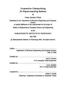
Data transfer is expensive: Communications between the host and device for large data streams can be effected at rates of up to 1-1.5 GB/s (publicity material calls for higher rates) over the PCI-express bus in which the device is installed. Transfers to the device are somewhat faster than readbacks. While this rate is impressive, this is slower than local memory access on either device or the host, and moreover during the process the GPU is not operating on computations for several clock cycles. As a result if a program needs updates and communications between the host and device during computations there is a significant dimunition in performance, and these should be minimized. Variable size matters: As is apparent from the architecture, to achieve good performance on this platform careful mapping is necessary. For example below we show the results of a call to the NVIDIA CUBLAS Matrix vector product routine in terms of time and speed up over a single CPU code, for sizes the are multiples of 128, and for sizes that are just one less than this optimal size. Even in this almost favorable case a decrease in the performance by a factor of 2 is seen.

2.2

Fortran programming on the CPU-GPU

We have in the past pursued mixed programming in Fortran-90, C/C++, and Matlab for various scientific computing applications, with the majority of our code written in Fortran-90, with the use of OMP for parallel processing on multi-core and multi-CPU environments. While we lack data on how widespread the use of Fortran is, we suspect that users of Fortran and/or Matlab form the plurality of major scientific computing users. There is also a substantial amount of existing code available in Fortran. The CUDA manual does not indicate support for Fortran, thereby making it difficult for this substantial community to gain from the advances in GPGPU. However, the CUBLAS manual does include some hints for performing mixed language programming with Fortran, including a way to call C-code wrapper functions that calls CU code for BLAS. In particular, to provide performance by minimizing memory transfers the wrappers have to be implemented in a “non-thunking” fashion (i.e., without unnecessary copying) with pointers to variables on the device.

5

1.E+01

Matrix-matrix multiplication on GPU (CUBLAS) y=ax3

1.E+00 3

Time (s)

y=bx 1.E-01

N =2M -1 N =2

M

a/b=2

1.E-02

1.E-03 1.E+02

1.E+03

1.E+04

Matrix size, N

Figure 1: Wall clock time for two real dense NxN matrix multiplications on GPU (GeForce 8800GTX). The filled circles show the time, for matrix sizes N = 2M , while the open circles correspond to N = 2M − 1 (M = 7, ..., 12).

3

Tools for development and porting on GPU processors

Psychology of scientific programmers: There are two somehow contradicting parts in the development of a program for solution a particular scientific problem. In the initial development phase, as the mathematical algorithm is being converted to code with bugs, the scientist (user) wants to have tools for “peek” and “poke” of variables and array elements, checking what is going on even with a single array entry (needing a capability to get and set some values, i.e., dereferencing of pointers), getting and setting values of arbitrary parts of allocated arrays, reshaping, etc. A good example of computational environment friendly to scientists is provided by Matlab interface. Also several high level languages, such as Fortran 90 are convenient for this. Second, the desire is that the program should run with high performance. As the GPU is employed to accomplish the second requirement, the first part, which requires transparency and ease of manipulations with parts of the arrays, becomes a major difficulty for users. Finally, we note that we consider as an important issue simplicity and closeness of the syntax of the operators interfacing CPU and GPU to the native language (Fortran) operators, to substantially reduce code conversion/and debugging time. Use of the heterogeneous CPU GPU architecture: As mentioned earlier, multi-slot mother boards which can accommodate two to four multicore CPUs, up to 8-16 GB of RAM and up to three 8800 GTX cards on available PCI-Xpress slots are available in the market for prices much less than $10K. Not all 6

problems can be effectively mapped to the GPU, and any real scientific computing code will have sections that will use the multiple CPU cores and sections that use the multiple GPUs for both computation and display of results. As such, it makes sense to think of a programming style where both the CPU and GPU use is controlled from the main application. Our goal is to encapsulate the manipulation of the GPU variables and functions in modules that provide interfaces to the CPU code. Our tools:

With the understanding that the performance of the GPU substantially depends on the

thread block size, number of multiprocessors employed, and even position of the elements in the arrays, we introduce the concept of device variables, which have sizes and allocations on the GPU to provide high performance operations. As the user may require arbitrary sizes and access to the parts of these variables, which necessarily reduces the performance, we provide tools for access to the parts of the variables, and also have standard procedures which operate with the entire variable or its properly sized and allocated part for good performance. In this case the user should not see (or should not care) that the actual device variable has a different size and allocation on the device, and in fact, the GPU may work with a larger array, which may be even differently allocated, which includes the user specified non-preferred sized part. We also understand that the first part of the scientific programming psychology mentioned above, is mostly applied to the debugging stage, while some minor manipulations with data allocated on the device can be made during high performance execution, if needed, to avoid unnecessary transfer of the whole array back and forth from GPU to CPU. This also may be used to “prepare” the array before high performance operation. To implement this concept it is not sufficient to describe the array with a single pointer, as, e.g., it is possible to do in CUBLAS with the non-thunking wrapper. Instead the device variable should be a structure, which encapsulates information about the pointer, size, and some other parameters, e.g., the type of variable, its dimensionality (vectors, matrices, 3d matrices, etc.), leading dimensions, allocation status, and so on. C and Fortran-90 provide convenient tools to work with structures, which for the user appear to be very similar to conventional C or Fortran syntax, while also allowing wrapping of function calls and overloaded functions suitable for the use with different types, shapes, and optional parameters. The CUBLAS functions also can be naturally wrapped and thus be much more convenient to use, as the user need not keep in mind what are leading dimensions of the variable, storage increments, and what kind of CUBLAS function he or she needs to call. This also avoids bugs due to calling errors. Also, the encapsulated variables provide shorter forms for calls of other library functions, such as CUFFT. For example, we have 1, 2 or 3 dimensional forward FFT can be called with a single function devf_fft(a), with optional variables plan, and b. In case no optional variables are specified this function creates the execution plan based on the type and shape of a and preforms an inplace FFT. If a plan is provided the execution is performed according to it, and if b is provided, then transform b=FFT(a) is performed. 7

Example of use:

Fig. 2 shows an example of code conversion for a subroutine in a package that is

used to solve a problem in plasma turbulence that is described in Section 4. Briefly, this code executes the timestepping in a homogeneous plasma turbulence simulation. Here the simulation is done in Fourier space, but the convective nonlinear terms are evaluated in real space pointwise, followed by a conversion to real space. As can be seen the source code in the original version (on the left) and the CUDA version (on the right) are very similar. However, all the variables on the right reside on the device. Moreover, all the commands on the right cause the operations indicated on the left to be applied to the variables on the device. Some pieces of the original code can be performed more efficiently if no thread synchronization is required and one custom function can be used instead of two (e.g., instead of two standard generic functions devf_mul we can use a single function devf_mul1, see Fig. 2). We also wish to point out that no CU or C code was needed to achieve this transformed routine (except that originally written for the module functions and precompiled to a static library). Modified Fortran Code

Original Fortran Code subroutine nlterms(isave,a,b,nl)

subroutine dev_nlterms(isave,dv_a,dv_b,dv_nl)

use com_module

use dv_com_module use mod_devObject

complex,dimension(:,:),intent(in) ::a,b complex,dimension(:,:),intent(out):: nl integer :: isave

type(devVar),intent(in) :: type(devVar),intent(out):: integer :: isave

if(isave /= 1) then kxa2=ikx*a kya2=iky*a call fftwnd_f77_one(plan_f,kxa2,kxa2) call fftwnd_f77_one(plan_f,kya2,kya2) endif

if(isave call call call endif

/= 1) then devf_mul1(dv_kxa2,dv_kya2,dv_ikx,dv_iky,a) devf_fft(dv_kxa2,fftplan) devf_fft(dv_kya2,fftplan)

if(isave /= 2) then kxb2=ikx*b kyb2=iky*b call fftwnd_f77_one(plan_f,kxb2,kxb2) call fftwnd_f77_one(plan_f,kyb2,kyb2) end if

if(isave call call call endif

/= 2) then devf_mul1(dv_kxb2,dv_kyb2,dv_ikx,dv_iky,b) devf_fft(dv_kxb2,fftplan) devf_fft(dv_kyb2,fftplan)

nl=kxa2*kyb2-kxb2*kya2 call fftwnd_f77_one(plan_b,nl,nl) nl=nl*scale

call devf_mul2(dv_nl,dv_kxa2,dv_kyb2,dv_kya2,dv_kxb2) call devf_ifft(dv_nl,fftplan) call devf_mul(dv_nl,dv_nl,dv_scale)

end subroutine nlterms

end subroutine dv_nlterms

dv_a,dv_b dv_nl

Figure 2: Example of code conversion using the developed modules. The subroutine evaluating the nonlinear term pseudospectrally is shown above. Our module declares data types for device variables and device functions, and provides a set of routines 8

for them. For device variables there are routines to allocate, to deallocate, to transfer data into them, copy data back from them, change their casts, etc. Currently we have functions for integer*4, real*4, and complex*4 variables, while the use of structures allows one to easily extend the types, without any visible change of the routines for the user. In addition code for performing simple data assignments on the GPU with zero, ones or random numbers is available for initialization statements. Convenient to use interfaces to the CUBLAS functions that avoid having to pass large numbers of parameters are also available. Treating double precision: Finally, while the GPU works with single precision variables, scientific computing on the CPU is usually done in double precision. To allow embedding of GPU calls in double precision code, we have developed module functions to allow the host real double precision and complex double precision variables to be transferred to the device, provided the data is within range, and with the inevitable loss of precision the conversion will cause. After computations are performed on the device the returned variables are automatically converted in the host code back to double precision. We had initially expected to write routines similar to those in [14, 40] to implement the double precision that is needed. However, NVIDIA has announced the availability of double precision on CUDA later in 2007. Accordingly it did not make sense for us to replicate this work. Instead we have followed an approach that assumes this structure and added placeholder code for double precision. Below we provide two examples of typical scientific problems for which existing Fortran codes were easily translated to interface with the GPU, and some performance results for test cases. The conversion in each case took less than two person-days.

4

Pseudospectral Simulations of Plasma Turbulence

Plasma (ionized gas) is a ubiquitous component of the universe, and almost all plasma is found to be turbulent. The theoretical framework that has been developed to study these essentially kinetic problems is known as “gyrokinetics.” [2, 17, 16, 25, 28] Gyrokinetics describes plasma as a collection of particles whose orbits are a combination of fast gyration in the background magnetic field, unconstrained motion along the magnetic field, and slow drifts across the field. The particles interact via Fokker-Planck collisions and through the electric and magnetic fields associated with their self-consistently evolving charge and current densities. Early simulations of gyrokinetic dynamics mainly used particle-in-cell algorithms.[30, 31, 34] More recently, pseudospectral techniques, which advance either a probability distribution function in phase space for each plasma species, fs = fs (x, v; t) or a few velocity-space moments of each distribution function in real space have advanced rapidly.[29, 10, 11, 36] Advances in closure models[26, 7] and in the development of simple fluid models of fully gyrokinetic systems[15, 37, 38] have kept interest in simulations of (complicated)

9

nonlinear fluid equations high. Fundamental aspects of gyrokinetic theory dictate certain features of any simulations in this area of research. In particular, the nonlinearities which arise are consistently of the Poisson bracket type, arising as they do from the peculiarities of charged particle motion in strong magnetic fields. Consider the simple example of the pure perpendicular convection of some passive scalar f by a long-wavelength, incompressible flow v: df ∂f =0→ + v · ∇f = 0. dt ∂t

(1)

ˆ, then the flow is the E × B flow, If the magnetic field is given by B = B0 z

v=

c cE × B ˆz × ∇Φ, = B02 B0

where Φ is the electrostatic potential, and c is the speed of light. The second term in Eq. (1) is

v · ∇f =

c c ˆ × ∇Φ · ∇f ≡ [Φ, f ], z B0 B0

where the Poisson bracket is defined by

[Φ, f ] ≡

∂Φ ∂f ∂f ∂Φ − . ∂x ∂y ∂x ∂y

(2)

If the potential Φ is not long wavelength, but instead varies on scales comparable to the radius of gyration of the plasma ions, then there are corrections to this motion. It can be shown, however, that the nonlinearities which arise remain of the Poisson bracket form. We now turn to a very simple model of plasma dynamics [37] in the plane perpendicular to the magnetic field, which has been shown to accurately describe the self-consistent generation of coherent, zonal flows by plasma turbulence in laboratory experiments. This example problem is set in a two-dimensional, periodic domain which models the cross-section of a “flux tube” of plasma. The model consists of equations for the local fluctuations of ion density and temperature, together with Poisson’s equation, which provides the self-consistent electric field from the ion density and temperature. The temperature plays a role in the theory because the fluctuations which the theory describes have wavelengths comparable to the typical ion radius of gyration. When the temperature T is (momentarily) higher, the radius of gyration is changed, and therefore the convection of the plasma by the fluctuating E × B flow is changed. In suitably normalized form, the

10

equations are ∂n τ + [φ, n] + [∇2⊥ φ, T ] = 0, ∂t 2 ∂T + [φ, T ] = 0, ∂t h τ i n = φ − φ¯ − ∇2⊥ (1 + τ )φ − τ φ¯ + T . 2

(3) (4) (5)

In these equations, τ is a parameter related to the plasma temperature, and the overbar represents an average R along the magnetic field. In the two-dimensional limit we consider here, φ¯ ≡ δ/Ly dy φ, where δ is either

zero or unity, depending on the application in mind. The physical importance of δ is obscure; here, we discuss its importance in the context of the mathematical model. We note in passing that the computational

complexity of this model is exactly equivalent to the widely used 2-D reduced magnetohydrodynamic model of Alfvenic plasma turbulence. Algorithm: We solve these equations with a standard second-order Runge-Kutta time advance, coupled with a pseudo-spectral evaluation of the nonlinear terms. The derivatives are evaluated in k−space, while the multiplications in Eq. (2) are carried out in real space. The standard 2/3 rule for dealiasing is applied, and small “hyperviscous” damping terms are added to Eqs. (3-4) to provide stability at the grid scale. This is required only because of the highly simplified nature of the model. We have calculated the stability and evolution of simple flows in this model with a standard CPU-based computer and with the combined CPU/GPU configuration. The results agree with analytic expectations[37] — namely, counter-propagating flows in the x−direction are strongly unstable to breakup and decay when δ = 1, but not when δ = 0. The results are the same on both configurations. Although this is a particularly simple model of magnetized plasma dynamics, it is one of many closely related mathematical cousins in a family of models of gyrokinetic physics. The basic algorithms demonstrated here on the CPU/GPU configuration can be immediately applied to more sophisticated plasma turbulence problems with laboratory and astrophysical applications.

5

Radial Basis Function Interpolation and Evaluation

While the BLAS type routines are very useful for large matrix operations and have efficient GPU analogs, another class of important algorithms are matrix-free, in the sense that the matrix entries are given by radial basis functions (or kernel functions) of the distance between members of a point set of size N . Thus instead ¡ ¢ of building the dense O N 2 radial-basis function matrix in some situations it is possible to just perform all actions of this matrix by creating the entry on the fly. This allows dealing with a large problem without 11

having to pay an O(N 2 ) memory penalty. Fast multipole methods allow one to perform matrix vector products with these matrices in O(N log N ) time but with considerable analytical and programming effort. Another possibility is to instead use the GPU hardware to evaluate the matrix vector product. Example applications include machine learning (sums of Gaussian and other kernel functions in high dimensions), N-body simulations in gravitational and molecular dynamics, radial basis function interpolation of implicit functions etc. Here we present speed up of a state-of-the art algorithm for RBF interpolation proposed by Faul et al. [19]. Interpolation of scattered data of various types using radial-basis functions has been demonstrated to be useful in different application domains [27, 8, 12, 41]. Much of this work has been focused on the use of £ ¤ polyharmonic, multiquadric and Gaussian radial-basis functions φ : Rd × Rd → R that fit data as s (x) =

N X

λj φ (|x − xj |) + P (x) ,

x ∈ Rd

(6)

j=1

where choices for φ include ⎧ ⎪ ⎪ r2n+1 ⎪ ⎪ ⎨ ¡ ¢1/2 φ (r) = r2 + c2 ⎪ ⎪ ³ ¡ ¢ ´ ⎪ ⎪ ⎩ exp − r 2 c

polyharmonic (R3 ) multiquadric (Rd )

.

Gaussian (Rd )

Here λj are coefficients while P (x) is a global polynomial function of total degree at most K − 1, which are necessary to fit the growing functions above. The coefficients {λ} and the polynomial functions P (x) are chosen to satisfy the N fitting conditions and constraints

s (xj ) = f (xj ) ,

j = 1, . . . , N ;

N X

λj Q (xj ) = 0,

j=1

for all polynomials Q of degree at most K − 1.The polynomial basis is usually taken to be just the constant, in which case the system of equations that needs to be solved to find the coefficients λ are ⎛

⎞⎛ ⎞ ⎛ ⎞ T Φ 1 λ f ⎜ ⎟⎜ ⎟ ⎜ ⎟ ⎝ ⎠⎝ ⎠=⎝ ⎠, 1 0 b 0

Φij = φ (xi − xj ) , i, j = 1, . . . , N ;

1 =1, 1, . . . , 1].

Micchelli [32] has shown that this system of equations is nonsingular. For large N, as is common in many applications, the computational time and memory required for the solution of the fitting equations is a significant bottleneck. Direct solution of these equations requires

12

¡ ¢ ¡ ¢ O N 3 time and O N 2 memory. Iterative approaches to solving this set of symmetric equations require

evaluations of dense matrix vector products Φλ which have a O(N 2 ) computational cost. Furthermore, for

rapid convergence of the iteration, the system must be preconditioned appropriately. Considerable progress in the iterative solution of multiquadric and polyharmonic RBF interpolation was made with the development of preconditioners using cardinal functions based on a subset of the interpolating points. This approach was first proposed by Beatson and Powell [3]. Recently, an algorithm was published by Faul et al. [19], which uses the cardinal function idea, and in which for each point a carefully selected set of q points was used to construct the preconditioner. In informal tests we found that this algorithm appears to achieve a robust performance, and was able to interpolate large problems in a few iterations, where other cardinal function based strategies sometimes took a large number of steps. However, its cost remains at O(N 2 ), and it requires O(N 2 ) memory. The purpose of this paper is the acceleration of this algorithm using GPUs. Similarly to many other iterative techniques the FGP05 algorithm can be accelerated if a Fast Multipole Method (FMM) for the matrix vector product required at each step is available, making the cost of each iteration O (N log N ) or so [22]. However, developing an FMM requires considerable analytical and programming skill. While the possibility of the use of the FMM was mentioned in [19], results were not reported. Fast multipole methods have been developed for various radial basis kernels including the multiquadric in Rd [13], the biharmonic and polyharmonic kernels in R3 [24], the polyharmonic kernels in R4 [6], and Gaussian kernels [23, 35]. Use of the FMM can thus reduce the cost of the matrix vector multiply required in each iteration of the FGP05 algorithm to O(N log N ). Graphics processors can significantly accelerate the matrix vector product (though not improve the asymptotic complexity), without this analytical load. Results based on the GPU based matrix-vector product are shown below.

6

Performance tests

We conducted some comparative performance tests for the problems described above. In both cases the serial Fortran code was compiled with Intel 9.1 compiler and launched on 2.67 GHz Intel Core 2 extreme QX 6700 (for the tests we employed only 2GB of RAM and one of four CPUs). Computations were performed in single precision. A single NVIDIA GeForce 8800 GTX (not connected to a display) was employed for runs involving CUDA programming and the encapsulation technology mentioned above. In the first case, related to the plasma simulations the initialization of the main time loop was performed on CPU then the loop was executed either on CPU or on GPU and the wall clock time was measured for 100 time steps of the algorithm. In both cases several complex forward and inverse FFTs on grids N × M were executed per time step, which was performed using the second order Runge-Kutta propagator. In the

13

1.E+02

y=ax2 y=bx2

1.E+01

Time (s)

CPU GPU 1.E+00 a/b=25 1.E-01 2D MHD Simulations (100 Time Steps in Pseudospectral Method) 1.E-02 1.E+01

1.E+02

1.E+03

1.E+04

N (equivalent grid (NxN)) Figure 3: Dependences of the wall clock time for execution of 100 time steps in the pseudospectral method for serial CPU implementation (the squares) and for the GPU (the circles).

tests we varied N from 16 to 1024 while by doubling the size for each next case, M was selected to be either N or 2N . Since the time should be a function of N M the cases when M 6= N are plotted in Fig. 3 for equivalent N = (N M )1/2 , and further under N we mean this equivalent N . We also measured the relative error in L∞ norm (point by point over the entire solution) after 100 steps on CPU and GPU, to check if the produced results are close enough. This error varied depending on the grid size, while stayed within the range 10−4 -10−3 for all cases and did not show any regular error growth or accumulation pattern. Fig. 3 illustrates comparison of the CPU and GPU wall clock times for solution of the same problem. Theoretically, the algorithm should be scaled as O(N 2 log N ), which is close to O(N 2 ) and the performance graphs show that this asymptotic complexity is achieved in both cases. However the CPU implementation starts to demonstrate scaling close to theoretical almost immediately, while the code running on the GPU achieves this pattern only for N ≥ 256, due to various overheads and time latency in the GPU multiprocessor loads. In log-log plot the theoretical curve looks like straight line. The shift between the lines corresponding to the two cases is a logarithm of the time ratio, which is about 25 for cases N ≥ 256. In other words, we obtained 25 times speedup of the 2D plasma/MHD pseudospectral algorithm using the GPU. 14

1.E+04

FGP'05 Algorithm y=ax2 (Iterative Solution of Dense RBF System)

1.E+03 CPU

y=bx2

Time (s)

1.E+02 GPU 1.E+01

1.E+00 a/b=15 1.E-01

1.E-02 1.E+02

1.E+03

1.E+04

1.E+05

Number of Sources, N Figure 4: Dependences of the wall clock time for iterative solution of the dense NxN linear system with on kernel matrix entry computations in the FGP’05 algorithm for the RBF fitting. Notations are the same as in Fig. 3.

The performance for the radial basis function interpolation is illustrated in Fig. 4, where the preconditioner was computed on the CPU, while only the performance when executing the iterative loop was analyzed. Here again, theoretically the algorithm should be scaled as O(N 2 ) if the number of iterations does not increase with N. However, in the case we ran we observed a slightly increase with N . Note then that the number of iterations to achieve the same convergence error, which in both cases was 10−6 was the same for CPU and GPU for N < 10000, while for larger N slight variations in favor of either the GPU or CPU implementation were randomly observed. In any case the difference was not more than 2 iterations. We also checked the error in different norms for the obtained solutions, which was small for relatively small N < 1000 while showed growing pattern for larger N . Such growth we observed also in other cases implemented on CPU, when the matrix-vector product is computed with some accuracy (e.g. using the FMM). In any case the relative error in L2 norm for random point distributions and random function values was of order 10−3 for the largest tested N = 32768, which is acceptable for many interpolation problems. Fig. 4 shows that close to theoretical scaling is observed for N ≥ 1000 in which case the speedup obtained due to the use of 15

GPU can be in the range 14-17.

7

Conclusions

We developed a pilot version of the interface to ease transfer and debugging of codes written in Fortran 9x to GPU, which employs CUDA, multilanguage Fortran/C++ environment for wrappers and operates with structures convenient for the user. These structures are designed to provide transparency on the debugging stage while still allowing one to develop high performance release versions. The developed interface was applied to implement and execute some typical algorithms appeared in scientific computing (pseudospectral method and multidimensional interpolation via the RBF) on GPU. Accuracy and speedups obtained in this way were analyzed and we achieved at least one order of magnitude speedups. As future work we consider opportunities to ease customization and extension of library functions and to use computational configurations of several CPU cores and GPUs. Of course, a similar approach can be applied to ease conversion of programs written in languages such as Matlab and C++ on the GPU.

References [1] NVIDIA Guide,

CUDA Version

Compute 0.8,

Unified

NVIDIA

Corp.

Device 2/2/2007.

Architecture (Available

Programming online

at

http://developer.download.nvidia.com/compute/cuda/0_8/NVIDIA_CUDA_Programming_Guide_0.8.pdf) [2] T. Antonsen and B. Lane, Phys. Fluids “Kinetic equations for low frequency instabilities in inhomogeneous plasmas.” 23, 1205 (1980). [3] R.K. Beatson and M.J.D. Powell, “An iterative method for thin plate spline interpolation that employs approximations to Lagrange functions,” In: D. F. Griffiths & G. A. Watson (eds), Numerical Analysis 1993, Longmans, Harlow, 1994, 17—39. [4] Pieter Bellens, Josep M. Perez, Rosa M. Badia and Jesus Labarta, “CellSs: a Programming Model for the Cell BE Architecture,” Proceedings, ACM/IEEE Supercomputing, 2006. [5] L. S. Blackford, J. Demmel, J. Dongarra, I. Duff, S. Hammarling, G. Henry, M. Heroux, L. Kaufman, A. Lumsdaine, A. Petitet, R. Pozo, K. Remington, R. C. Whaley, An Updated Set of Basic Linear Algebra Subprograms (BLAS), ACM Trans. Math. Soft., 28-2, pp. 135—151 (2002). [6] R. K. Beatson, J. B. Cherrie, and D. L. Ragozin, “Fast evaluation of radial basis functions: Methods for four-dimensional polyharmonic splines”, SIAM J. Math. Anal., 32(6), 2001, 1272-1310. 16

[7] M. A. Beer and G. W. Hammett, “Toroidal Gyrofluid Equations for Simulations of Tokamak Turbulence, ” Phys. Plasmas 3, 4046 (1996). [8] J. Bloomenthal, C. Bajaj, J. Blinn, M.P.Cani-Gascuel, A. Rockwood, B. Wyvill, and G. Wyvill, Introduction to Implicit Surfaces, Morgan Kaufmann Publishers, San Francisco, CA, 1997. [9] Ian Buck, Tim Foley, Daniel Horn, Jeremy Sugerman, Kayvon Fatahalian, Mike Houston, Pat Hanrahan Fatahalian, Mike Houston, Pat Hanrahan, Brook for GPUs: Stream Computing on Graphics Hardware, International Conference on Computer Graphics and Interactive Techniques archive, ACM SIGGRAPH Courses, article 109, 2005. [10] J. Candy and R. E. Waltz, “Anomalous Transport Scaling in the DIII-D Tokamak Matched by Supercomputer Simulation, ” Phys. Rev. Lett. 91, 045001 (2003). [11] J. Candy and R. E. Waltz, “An Eulerian Gyrokinetic Maxwell Solver, ” J. Comp. Phys. 186, 545 (2003). [12] J.C. Carr, R.K. Beatson, J.B. Cherrie, T.J. Mitchell, W.R. Fright, B.C. McCallum, and T.R. Evans, “Reconstruction and representation of 3D objects with radial basis functions,” ACM SIGGRAPH 2001, Los Angeles, CA, 2001, 67-76. [13] J. B. Cherrie, R. K. Beatson, and G. N. Newsam, “Fast evaluation of radial basis functions: Methods for generalized multiquadrics in Rn ”, SIAM J. Sci. Comput. , 23(5), 2002, 1549-1571. [14] T. Dekker, A floating-point technique for extending the available precision. In Numerische Mathematik 18, 224-242. (1971) [15] W. Dorland, F. Jenko, M. Kotschenreuther, and B. Rogers, “Electron Temperature Gradient Turbulence ” Phys. Rev. Lett. 85, 5579 (2000). [16] D. H. E. Dubin, J. A. Krommes, C. Oberman, and W. W. Lee, “Nonlinear Gyrokinetic Equations.”, Phys. Fluids 26, 3524 (1983). [17] E. A. Frieman and L. Chen, “Nonlinear Gyrokinetic Equations for Low-Frequency Electromagnetic Waves in General Plasma Equilibria ”, Phys. Fluids 25, 502 (1982). [18] Matteo Frigo and Steven G. Johnson, “The Design and Implementation of FFTW3,” Proceedings of the IEEE 93 (2), 216—231 [19] A. C. Faul, G. Goodsell, M. J. D. Powell, “A Krylov subspace algorithm for multiquadric interpolation in many dimensions,” IMA J. Numer. Anal., 25, 2005, 1—24. 17

[20] Nico Galoppo, Naga K. Govindaraju, Michael Henson, Dinesh Manocha, “LU-GPU: Efficient Algorithms for Solving Dense Linear Systems on Graphics Hardware,” Proceedings IEEE/ACM SuperComputing, 2005. [21] Naga K. Govindaraju, Scott Larsen, Jim Gray, Dinesh Manocha. “A Memory Model for Scientific Algorithms on Graphics Processors,” Proceedings IEEE/ACM Supercomputing, 2006. [22] L. Greengard and V. Rokhlin, “A fast algorithm for particle simulations,” J. Comput. Phys., 73, 1987, 325-348. [23] L. Greengard and J. Strain, “The fast Gauss transform,” SIAM J. Sci. Statist. Comput., 12, 1991, 79— 94. [24] N.A. Gumerov and R. Duraiswami, “Fast multipole method for the biharmonic equation in three dimensions,” J. Comput. Phys., 215(1), 2006, 363-383. [25] T. S. Hahm, W. W. Lee, and A. Brizard, “Nonlinear Gyrokinetic Theory for Finite-Beta Plasmas ” Phys. Fluids 31, 1940 (1988). [26] G. W. Hammett and F. W. Perkins, “Fluid Models for Landau Damping with Application to the IonTemperature-Gradient Instability, ” PRL 64, 3019 (1990). [27] R. L. Hardy, “Theory and applications of the multiquadric-biharmonic method,” Comput. Math. Appl., 19, 163—208, 1990. [28] G. G. Howes, S. C. Cowley, W. Dorland, G. W. Hammett, E. Quataert, and A. A. Schekochihin, “Astrophysical gyrokinetics: Basic equations and linear theory, ”Ap. J. 651, 590 (2006).. [29] M. Kotschenreuther, W. Dorland, G. W. Hammett, and M. A. Beer, “Quantitative predictions of tokamak energy confinement from first-principles simulations with kinetic effects, ” Phys. Plasmas 2, 2381 (1995). [30] W. W. Lee, “Gyrokinetic Approach in Particle Simulation, ” Phys. Fluids 26, 556 (1983). [31] W. W. Lee, “Gyrokinetic Particle Simulation Model, ” J. Comput. Phys. 72, 243 (1987). [32] C. A. Micchelli, “Interpolation of scattered data: distance matrices and conditionally positive definite functions.” Constr. Approx., 2, 1986, 11—22. [33] John D. Owens, David Luebke, Naga Govindaraju, Mark Harris, Jens Krüger, Aaron E. Lefohn, and Timothy J. Purcell, “A Survey of General-Purpose Computation on Graphics Hardware,” Proceedings EUROGRAPHICS 2005, pp. 21-56, 2005. 18

[34] S. E. Parker and W. W. Lee, “A Fully Nonlinear Characteristic Method for Gyrokinetic Simulation, ” Phys. Fluids B 5, 77 (1992). [35] V.C. Raykar, C. Yang, R. Duraiswami, and N.A. Gumerov. “Fast computation of sums of Gaussians in high dimensions,” Tech. Report CS-TR-4767, Department of Computer Science, University of Maryland, 2005. [36] P. Ricci, B. N. Rogers, and W. Dorland, “Small-scale turbulence in a closed-field-line geometry, ” Phys. Rev. Lett. 97, 245001 (2006). [37] B. N. Rogers, W. Dorland, and M. Kotschenreuther, “The Generation and Stability of Zonal Flows in Ion Temperature Gradient Mode Turbulence, ” PRL 85, 5536 (2000). [38] B. N. Rogers and W. Dorland, “Noncurvature-driven modes in a transport barrier, ” Physics of Plasmas 12, 062511 (2005). [39] M. Segal and M. Peercy, “A Performance-Oriented Data-Parallel Virtual Machine for GPUs,” Proceedings of Siggraph [40] Andrew Thall, “Extended-Precision Floating-Point Numbers for GPU Computation,” International Conference on Computer Graphics and Interactive Techniques archive Research posters, ACM SIGGRAPH 2006. [41] G. Turk and J.F. O’Brien, “Modelling with implicit surfaces that interpolate,” ACM Trans. on Graphics, 21(4), 2002, 855-873 [42] Juekuan Yang, Yujuan Wang, Yunfei Chen, “GPU accelerated molecular dynamics simulation of thermal conductivities,” Journal of Computational Physics 221 (2007) 799—804 (2005).

19