Efficient Simulation of Temperature Evolution of Overhead Transmission Lines Based on Analytical Solution and NWP Rui Yao, Kai Sun, Senior Member, IEEE, Feng Liu, Member, IEEE, and Shengwei Mei, Fellow, IEEE 1 Abstract
--- Transmission lines are vital components in power systems. Tripping of transmission lines caused by over-temperature is a major threat to the security of system operations, so it is necessary to efficiently simulate line temperature under both normal operation conditions and foreseen fault conditions. Existing methods based on thermal-steady-state analyses cannot reflect transient temperature evolution, and thus cannot provide timing information needed for taking remedial actions. Moreover, conventional numerical method requires huge computational efforts and barricades system-wide analysis. In this regard, this paper derives an approximate analytical solution of transmissionline temperature evolution enabling efficient analysis on multiple operation states. Considering the uncertainties in environmental parameters, the region of over-temperature is constructed in the environmental parameter space to realize the over-temperature risk assessment in both the planning stage and real-time operations. A test on a typical conductor model verifies the accuracy of the approximate analytical solution. Based on the analytical solution and numerical weather prediction (NWP) data, an efficient simulation method for temperature evolution of transmission systems under multiple operation states is proposed. As demonstrated on an NPCC 140-bus system, it achieves over 1000 times of efficiency enhancement, verifying its potentials in online risk assessment and decision support. Index terms --- Transmission line temperature, dynamic line rating, situational awareness, numerical weather prediction (NWP), kmeans clustering, analytical solution, N-k contingency analysis.
I. INTRODUCTION
T
RANSMISSION lines play vital roles in conveying electricity from the plants to the users in the power systems [1]. Also, overhead transmission lines cover largest area across the system, and they are exposed to complicated environmental conditions [2]. Many kinds of natural events threat the transmission lines in operations, such as lightning, strong wind, hot weather, etc. [3, 4]. A transmission line has certain thermal capacity, and once the temperature exceeds limit, the line may face risk of tripping due to sagging and tree contact [5, 6] or quitting into maintenance due to heat damage [7]. Such threats are particularly prominent on heavy-duty lines exposed to high ambient temperature and low wind conditions. The outage of transmission lines due to over-temperature is a major cause of cascading outages in power systems (e.g. the 1996 WSCC outages [8] and 2003 US-Canada blackout [9]). Moreover, the fast-growing load and developing electricity market but relatively slow upgrade of transmission infrastructure have pushed transmission lines toward operational limits [10].
This work was supported by the CURENT Engineering Research Center. R. Yao and K. Sun are with the Department of EECS, University of Tennessee, Knoxville, TN 37996, USA (emails:
[email protected],
[email protected]). F. Liu and S. Mei are with the State Key Laboratory of Power Systems, Department of Electrical Engineering, Tsinghua University, Beijing 100084, China. (email:
[email protected],
[email protected]).
Therefore, it is necessary to enhance the situational awareness of transmission lines under various environmental conditions [11]. Specifically, it is desirable to realize accurate and efficient simulation of future transmission-line temperature evolution (TLTE) by considering environmental factors. To exploit the transmission capacity and to monitor the lines, the dynamic line rating (DLR) is proposed to determine the maximum flow under which the steady-state temperature will not exceed limit [12]. However, the DLR only studies steady state temperature. In fact, it is also important to address the temperature transients to obtain more accurate and panoramic information of the risk of the transmission system over a timespan. Besides normal operating conditions, it is also necessary to study other operation states, e.g. when the system is under contingencies. This is particularly useful and adds to robustness of system in case the system is under maintenance, or operators are unaware of loss of components due to malfunctions in the SCADA/EMS [9], or when the system is under cyberattacks [13]. IEEE [14] and CIGRE [15] proposed models describing TLTE. An existing approach to simulating the TLTE is numerical integration on the differential equation. However, such an approach requires huge computational efforts and is computationally difficult in system-wide analysis because: 1) a line should be divided and simulated in many segments since the environmental parameters are different along the line; 2) when system state changes (e.g. simulation under a different contingency), a complete system-wide simulation is required. To overcome the limitations of conventional numerical methods, this paper first derives an approximate analytical solution of TLTE. The proposed approximate analytical solution can significantly improve the efficiency of simulation and enhance the practicality of overall operational monitoring and analysis of transmission lines in four folds: 1) The approximate analytical solution significantly improves the efficiency of simulating TLTE by simply assigning values to variables of the analytical expression. 2) This paper proposes a method for fast updating the analytical solution when current changes, which further enhances computational speed in batch analysis of multiple operation states (e.g. analysis of a set of contingencies). 3) Metrics useful for the security analysis and decisionmaking can be derived from the analytical solution, e.g. the time for a conductor to reach the temperature limit. 4) The analytical solution can be further utilized in more advanced risk modeling and analysis for transmission systems. Moreover, this paper uses the high resolution numerical weather prediction (NWP) service as the source of environmental data. The NWP has become a mature public service providing with reliable wide-area, high-resolution
environmental data, which also has potentials in power system applications [16]. In the US, the NWP previously only provides an hourly forecast, which is too coarse to meet the temporal resolution for the simulation of transmission line temperature [17]. Recently the High-Resolution Rapid Refresh (HRRR) model has been put into operations starting from August 2016, providing an hourly-refreshed forecast at the 15-minute interval and 3km resolution covering contiguous US (CONUS) and Alaska with outreach of 18 hours [18]. Thus, the NWP turns out to be a promising source of environmental data for monitoring and assessment of real-time transmission line reliability. In this paper, with the analytical solution of TLTE and NWP as the source of environmental data, efficient system-wide simulation of TLTE is realized. Our method periodically retrieves environmental data and simulates system-wide TLTE [19] within the time coverage of NWP. With approximate analytical solutions and fast updates of solutions for the current operating condition, the proposed method is over 1000 times faster than conventional methods. Moreover, for lines with potential risks of over-temperature, we can also realize further analyses, e.g. estimating the risk of over-temperature by considering uncertainty of environmental factors and deriving the permissible time for remedial actions before overtemperature [20]. These results can be visualized in a space on environmental parameters to facilitate analysis and decision support for planning and operation. In the rest of the paper, section II derives the approximate analytical solution of TLTE. Section III applies analytical solutions into system-wide analysis of over-temperature events combing NWP data. Section IV verifies the accuracy and practicality of the method on a single conductor model, and section V demonstrates the accuracy and efficiency of systemwide simulation in NPCC system. Section VI draws conclusions.
II. ANALYTICAL SOLUTIONS OF LINE TEMPERATURE A. Model of TLTE Per the IEEE-738 standard [14], the TLTE follows the following differential equation: dT (1) mC p c qi qs qc qr dt where mC p is the heat volume per length of the conductor; Tc is the temperature of conductor and qi I 2 R(Tc ) is the joule heat generated by current I on a temperature-dependent resistance R(Tc ) R0 R (Tc T0 ) ; qs is the power of heat absorbed from sun light radiation as calculated by qs Qse sin( ) A , arccos[cos( H c ) cos( Zc Zl )] (2) Here, is absorptivity coefficient of the conductor; Qse is the solar radiation power per unit area; A is the projected area of conductor per unit length; H c is the sun altitude angle, and Zc and Zl are azimuths of the sun and line. In (1), qr is the radiation heat emitted from the conductor. T 273 4 Ta 273 4 (3) qr 17.8 D c (W/m) 100 100 where, is emissivity coefficient of the conductor; D is the diameter (mm); Ta is ambient temperature (°C). qc in (1) is the power of convection heat loss given by: qc max{qch , qcl , qcs } (4) h l s where, qc , qc and qc correspond to different wind speeds
(5) qch 0.754 K a N R 0.6 k f (Tc Ta ) (W/m) l 0.52 (6) qc K a [1.01 1.35 N R ]k f (Tc Ta ) (W/m) (7) qcs 3.645 f 0.5 D 0.75 (Tc Ta )1.25 (W/m) K a relates to the angle between wind and line [0 ,90 ] (8) Ka 1.194 cos 0.194cos 2 0.368sin 2 and k f is thermal conductivity of air. N R is Reynolds number N R ( D f Vw ) / f (9) where Vw is wind speed, f is air density, and f is air viscosity. k f , f and f are dependent on Tc and Ta [14]. B. Approximate analytical solution Next, we derive the approximate analytical solution of TLTE. Based on (2)-(9), (1) can be reformulated as dTc Qsi (Tc , Ta , I ,Vw , w , H c , Z c , Z l )(Tc Ta ) (10) dt where w is wind direction. is 2 2 17.8 D Tc 273 Ta 273 Cc I 2 R 10000 100 100 (11) (Tc ) mC p where term Cc comes from convection heat Cc max{0.754K a N R 0.6 k f , K a (1.01 1.35N R 0.52 )k f , 3.645 f 0.5 D0.75 (Tc Ta ) 0.25 }
(12)
The term Qsi is Qsi
I 2 R (Ta ) qs (Qse , H c , Z c , Z l ) mC p
(13)
Vw , w , Ta , H c , Zc , I and Qse can be regarded as constants (e.g. average value) over a period. This is generally reasonable since the heat volume of the conductor acts as a low-pass filter that suppresses the high-frequency fluctuation of parameters. Let T Tc Ta and denote as the function of new variable T , i.e. (T ) , then (10) is transformed as d T (14) Qsi (T )T dt Tests show that in most cases, (T ) has good linearity with T as illustrated in Fig. 1, so it can be approximated by (T ) 0 T T (15)
Fig. 1. The linearity of βΔ(ΔT) to ΔT. Conductor: Drake (diameter 28.1mm), July 1st, N30, line direction E-W, Vw=1.3m/s, wind direction E-W, Ta=40°C.
Thus, equation (14) is approximated as a constant-coefficient Ricatti equation (16) with solution (17). d T (16) Qsi 0 T T T 2 dt AC e T ( A B )t TcRic (t ) B Ta (17) 1 C e T ( A B )t where
B Te Ta , A B
0 Te Tc 0 , C T A Tc 0 Ta
(18)
Here Tc 0 is initial temperature, and Te is the steady-state temperature calculated by assuming dT/dt=0 in (16). Thus, the approximate analytical solution of TLTE is obtained, whose advantages are twofold: 1) the line temperature variation can be calculated efficiently, avoiding directly integrating (1) like conventional numerical methods; 2) the analytical formulation can conveniently be used in system risk assessment. Moreover, it is desirable to obtain an even simpler form as the solution of a first-order differential equation. Tcsimp (t ) Te (Tc 0 Te )e t (19) The aim is to find so that Tcsimp (t ) is not lower than TcRic (t ) and their difference is as small as possible. It is proved that the optimal is
T ( A B ) 02 4Qsi T
(20)
The first-order solution guarantees conservativeness, and the difference between Tcsimp (t ) and TcRic (t ) is restricted by
1 (t )
1 C
2
Te Ta A (21) 1 C C. Algorithms for obtaining analytical solution To obtain an analytical solution, first we solve the steady-state temperature Te with the Newton-Raphson (N-R) method as follows. At steady-state temperature, the equality holds: Qsi (Te ) Te 0 (22) where Te Te Ta . In most cases, from initial temperature Tc 0 to steady-state temperature Te , does not change much, so we can approximate (Te ) (Tc 0 ) . Then from (14) the steadystate temperature is approximated by (23) leading to a mismatch on the left-hand side of (24), denoted by Q. Qsi Tˆe (23) (Tc 0 ) 0 Tcsimp (t ) TcRic
Q Qsi (Tˆe ) Tˆe
(24)
Then we have (Tˆ ) (Tc 0 ) ˆ d d Q (Tˆe ) Tˆe (Tˆe ) e Te (25) dTˆ dTˆ Tˆ T e
e
e
Te , 0 , T and Qsi are calculated by (22)-(28) under current
I (namely the reference current). When current changes to I , note that T / T and / T does not depend on I according to (11), so approximately T ( I ) T ( I ) , and ( I 2 I 2 ) R Ta (29) Qsi ( I ) mCp ( I 2 I 2 ) R (30) mCp From (22), the steady-state temperature under current I can be estimated by
0 ( I ) 0 ( I )
Te ( I )
0 2 ( I ) 4 T ( I )Qsi ( I ) 0 ( I ) Ta 2T ( I )
(31)
Then the TLTE under new current I can be updated with (17) and (19). It indicates that only one N-R iteration is required if the environmental factors remain unchanged. The analytical update of line current will be very useful in batch analysis of multiple operation states (e.g. N-k contingency analysis), in which only line current is changed and the new solutions can directly be updated from (29)-(31).
III. EVALUATION OF OVER-TEMPERATURE EVENTS A. Sources of environmental data 1) NWP and historical data TABLE I. ENVIRONMENTAL DATA SOURCE AND UNCERTAINTY Operation Scheduling Planning
Source Uncertainty Source Uncertainty Source Uncertainty
NWP NWP Error Historical data/NWP Historical data distribution/NWP Error Historical data Historical data distribution
TABLE II. NOAA NWP MODEL SPECIFICATIONS Models
CFS
GFS
Coverage
Global
Global
Outreach Refresh Time-step Resolution
9 mo. 6 hr. 6 hr. ~56 km
16 days 6 hr. 3 hr. ~28 km
NAM North America 3.5 days 6 hr. 3 hr. ~12km
RAP North America 21 hr. 1 hr. 1 hr. ~13km
HRRR CONUS, Alaska 18 hr. 1 hr. 15 min. ~3km
c 0
The Newton-Raphson correction on Tˆe is
d Q (26) dTˆe Perform steps (24) to (26) repeatedly until the heat power mismatch becomes less than a given threshold, i.e. Q Q . Converged Te derives steady-state temperature Te Te Ta . The other parameters in the analytical solution can be derived: (T ) (Tc 0 ) T e (27) Te Tc 0 Tˆe Q
0 (Tc 0 ) T (Tc 0 Ta )
(28) Following the above steps to obtain Te , 0 and T , then the analytical solutions are derived based on (17)-(20). D. Efficient update of solution under different line currents The importance of the approximate analytical solution is in not only obtaining the TLTE efficiently but also efficiently updating solutions when system states change. Assume the environmental variables Vw , w and Ta to remain the same, and
Calculating the system-wide TLTE requires reliable sources of environmental data, mainly including ambient temperature, wind speed and wind angle. Table I shows data sources and uncertainties in different applications including planning, scheduling and operations. In operations, environmental data can be obtained from the numerical weather prediction (NWP) analysis and forecast results, and the uncertainty mainly comes from the error of the NWP [21]. Major NWP models used in the US are listed in Table II. The scheduling of power systems can vary on a daily or weekly basis, or even on monthly basis. Due to the limitation of NWP spatial resolution and time outreach, the NWP data can only cover up to weekly scheduling, and the error grows with the increase of NWP outreach. Therefore, longer-term scheduling will depend more on historical data, and the environmental data will have larger uncertainties. The historical environmental data can be collected from weather observations and/or the analysis of historical NWP results [22]. 2) Terrain effects
Take the NWP services in North America as an example. The environmental data such as near-surface temperature (2m altitude temperature) and wind speed (10m altitude wind x- and y-component) are available with spatial resolution as high as 3km (HRRR). The operational HRRR has enhanced the accuracy of near-surface prediction by considering terrain factors, yet such spatial resolution in some cases still cannot sufficiently reflect the terrain of smaller scales (e.g. small hills, valleys). Terrain has non-negligible impacts on environmental factors, especially on wind speeds and directions. More detailed terrain data are helpful to further improve the accuracy of simulation [23]. The correction of wind data considering even higher terrain resolution can be achieved with applications such as WindNinja [24], which is capable of recognizing terrain from web map services and utilizing NWP results to generate terrain-corrected wind vectors at spatial resolution of around 100m. Due to the limitation of space, in this paper we only use the HRRR forecast results as environmental parameter sources. The NWP results can also be further corrected using higher-resolution terrain as input data to the simulation of TLTE. B. Simulation of system-wide TLTE The proposed analytical solutions can be utilized in TLTE under either normal operating conditions or contingencies. Take the contiguous US and Alaska as examples. The high-resolution NWP service (RAP+HRRR) is covered. NWP data is open access to the public and can be retrieved from the NOAA Operational Model Archive and Distribution System (NOMADS). Since the line temperature largely depends on the environmental factors, the transmission line should be divided into segments in the analysis. For the HRRR resolution of 3km, the length of a line segment should not exceed 3km. However, if high-resolution terrain correction is adopted, the wind data will have much higher spatial resolution. To avoid diving too many line segments, the riskiest wind scenario (e.g. having the lowest wind speed) is for the line segment corresponding to the NWP spatial resolution. To further accelerate computation, the line segments with close positions and similar environmental factors can also be approximately regarded as the same, and then the parameters of analytical solutions can be regarded as the same. This paper also realizes line segment clustering (LSC) with K-means method [25]. Then the analytical solution parameters within a cluster can be regarded as the same and can be computed only once, further reducing computational burden. The parameters of LSC are the geographical coordinates, ambient temperature, wind speed, wind direction, line segment direction, and conductor type. The efficient system-wide simulation of TLTE can be realized with the proposed method. The NWP data are collected hourly. Assume the studied system states (e.g. post N-k contingency states) have been obtained. Then for each operational state and each line segment, an analytical temperature trace for up to 18 hours is obtained, as illustrated in Fig. 2. Note that the actual outreach of TLTE prediction will be a bit less than 18 hours. It is because the data assimilation of NWP needs to collect current observations and combine them with forecasts from the previous cycles to produce new forecasts, which generally takes about one hour (indicated by the shadowed areas along the timeline shown in Fig. 2). Therefore, the NWP data starting at time t0 will be ready at about an hour after t0 , and the real outreach of line temperature traces is about 17 hours. Such time outreach
should be enough for online decision support against overheat of transmission lines.
Fig. 2. Computation cycle in online operation.
C. Estimating the risk of over-temperature 1) Over-temperature risk at steady state The analytical solution can also facilitate further study of lines of interest (e.g. heavy-duty lines with higher risk of overheat). For example, we can investigate the risk of exceeding a temperature limit Tth considering uncertainties in environmental data. The steady-state temperature Te is determined by the ambient temperature Ta , wind speed Vw and direction angle w . Given Ta and w , the wind speed corresponding to steady-state temperature reaching Tth can be uniquely determined. When Te Tth , the convection heat is determined from (1): qc (Tth , Ta ,Vw , w ) I 2 R(Tth ) qs qr (Tth , Ta ) (32) s If qc (Tth , Ta ,Vw , w ) qc then Tth cannot be reached. Otherwise, we can intersect two wind speeds from qcl and qch : 1
qc (Tth , Ta , Vw , w ) 1.01 0.52 f V 1.35 K k (T T ) 1.35 D angle f th a 0 f l w
qc (Tth , Ta , Vw , w ) Vwh 0.754 K k (T T ) angle f th a
1 0.6
(33)
f D0 f
Then the smaller one of them, i.e., Vwth min{Vwh ,Vwl } , is the estimated maximum wind speed to cause over-temperature. Since Vwth corresponds to Tth , any wind speed lower than Vwth will result in steady-state temperature higher than Tth . Hence, Vw Vwth is the region of potential over-temperature events in the environmental parameter space. Given the marginal distribution of Vwth , the over-temperature probability can be estimated by Pr{Te Tth | Ta , w } Pr{Vw Vwth | Ta , w } FVw |Ta ,w (Vwth ) (34) where FVw |Ta ,w () is the marginal CDF of wind speed. In the environmental parameter space S p , the overall probability that steady-state temperature exceeds limit can be estimated by integration over the space of w and Ta . Pr{Te Tth } FVw |Ta ,w (Vwth ) p(Ta , w )d Sp
F
Vw |Ta , w
Ta ,
(Vwth ) p(Ta , w ) Ta w
(35)
w
2) Assessing the time to over-temperature Besides the risk that steady-state line temperature exceeds the limit, the transient as well as the time for the line temperature to rise to the limit are also desirable because it indicates the time left for the operators to take remedial actions to relief overheat.
Given Ta and w , and any Te between the maximum possible steady-state temperature Te max (obtained from the possible minimum wind speed Vw min ) and Tth , the time t for reaching Tth is calculated by the following procedure: Step 1. Calculate e Qsi / (Te Ta ) . Step 2. Calculate convection heat at the steady state. qc (Te , Ta ,Vw , w ) I 2 R(Te ) qs qr (Te , Ta )
the Drake ACSR [14]. First we demonstrate the results of TLTE calculation by comparing different analytical solutions with the results obtained by the numerical method. Related parameters are listed in Table III.
Step 3. Calculate Vwth from qc (Te , Ta ,Vw , w ) with (24). Step 4. Calculate (Tc 0 ) , T (e (Tc 0 )) / (Te Tc 0 ) ,
0 (Tc 0 ) T (Tc 0 Ta ) , and 02 4Qsi T Step 5. Calculate time to Tth with the first-order solution: 1 T T t ln e c 0 Te Tth Or one can derive it from a second-order analytical solution: 1 T T T T 0 / T 2Ta t ln e c 0 th e Te Tth Tc 0 Te 0 / T 2Ta All the points of t form a region indicating how much time is left for the conductor to reach Tth in the space of environmental parameters. Such results can be conveniently visualized and thus can enhance situational awareness of transmission lines and facilitate decision support against overheat.
IV. TESTS OF THE CONDUCTOR MODEL A. Verification of approximate analytical solutions Firstly, we test the derivation of steady-state temperature by using the N-R iteration described by (22)-(26). We set 50000 instances with various parameters: line diameters vary from 0.5cm to 4.75cm (covering all standard ACSRs); initial temperature from 20°C to 100°C; ambient temperature from 0°C to 40°C; line current from 0 to 200% of the nominal current; wind speeds from 0 to 10m/s. All the cases with steady-state temperatures below 300°C converge with respect to a tolerance Q 106 W/m . Over 95% cases converge within 10 iterations (Fig. 3). All the 50000 instances only cost 1.166s time in total.
Fig. 4. Comparison of analytical solutions with numerical results.
Set the current as I 800A and compare the solutions given by conventional numerical integration, the solution of Ricatti equation (17) and the first-order solution (19), as shown in Fig. 4. Both analytical solutions match well with the numerical result. The errors of analytical solutions compared with numerical integration solution are presented in Table IV. The Riccati equation solution gives negative errors, which means slightly lower temperature than numerical results (i.e. T ) and time lag of reaching a certain temperature (i.e. t ). While first order equation can guarantee conservativeness of results, which almost only gives limited positive error compared with numerical results. The accuracy and conservativeness of the first-order solution is desirable for security analysis. With a satisfactory accuracy, a simpler form than the Ricatti equation solution, and a higher efficiency than the numerical method, the first-order analytical solution is appealing in online simulation of TLTE and promising for a higher-level risk assessment. TABLE IV. ERRORS OF ANALYTICAL SOLUTIONS
maxδT+ (°C) maxδt+ (s) maxδT- (°C) maxδt- (s)
Ricatti eq. solution 0 0 0.5548 42.2
First-order solution 1.9938 72.8 0.0017 23.5
B. Analytical solutions by updating line current
Fig. 3. Steady state temperature iteration times. TABLE III. PARAMETERS FOR TEMPERATURE VARIATION CALCULATION Parameter Wind speed Wind direction Latitude Date Time Line direction Ambient temperature Initial temperature
Value 0.8m/s 90°(East) 30°N July 1st 12:00am 90°(W-E) 40°C 50°C
Then we test the accuracy of analytical solutions on a typical model of transmission line conductor. The tested conductor is
Fig. 5. Error of line temperatures under different current values.
With an analytical solution in which the parameters are obtained from the N-R iterations of (22)-(26), solutions at other line current values can be approximated from (29)-(31). Fig. 5 demonstrates the accuracy of simulating TLTE under different currents. The suggested ampere rating of the conductor is around 1000A. There are two curves corresponding to reference currents as 1500A and 1800A, respectively. From the result, before the current reaches the 1500A reference, the error is maintained below 1.5°C, while beyond 1500A, the error rises sharply. So another reference current is needed if the current can reach 2000A. With supplemented reference current as 1800A, the error
in the 0-2000A range is limited under 1.5°C. Extensive tests on various conductor models show that within 0-200% loading region, at most two reference current values are required to limit the error under 2°C. Since normally the protection setting point is around the 200% loading level, this method can generally cover the common long-term operating states of transmission lines. Because updating current values avoids re-calculation of N-R iterations, the computational efficiency is greatly enhanced. C. Over-temperature region of sample line segment Considering the uncertainty of the environmental factors, the probability of steady-state over-temperature events can be evaluated as discussed in III.C. The wind is assumed to follow Weibull distribution, as shown in the wind rose in Fig. 6. The ambient temperature is assumed to follow uniform distribution between 30°C and 40°C.
Fig. 7a, with x- and y-axes as wind direction and wind speed. The region is calculated efficiently following the methods in III.C.2 (only 1/4 of the region needs computation due to the symmetry in wind direction). Such a region can conveniently indicate the time left before the conductor temperature reaches the limit, i.e. the time for taking control actions to relieve overheat before it occurs. The time-to-over-temperature region can also be combined with the probability distribution of environmental factors, as shown in Fig. 7b. The contour plot masked over the region is the probability density of corresponding wind direction and speed. In Fig. 7b transparency is masked over the region to highlight the more possible environmental parameters as well as the corresponding time-to-over-temperature characteristics. V. APPLICATION IN NPCC SYSTEM We test the method on the NPCC 140-bus, 233-line system located in the northeast of the US and Canada. In this case, we assume the types of the conductors are set as in Table VI. TABLE VI. TYPICAL TRANSMISSION LINE CONDUCTOR SPECIFICATION [6] Voltage 765kV 500kV 345kV 230kV 138kV
Fig. 6. An example wind rose.
The binning of probability distribution of environmental factors affects both the accuracy and computational efficiency. In this case, 2-D binning of ambient temperature and wind direction is needed. Table V demonstrates the estimated probability and computation time under different binning densities. It shows that even with the coarsest 2525 binning, the result still does not deviate much (around 3%) from the 500500 binning. The results verify that the probability of overtemperature can be efficiently estimated with satisfactory accuracy. The method can be utilized for risk assessment in both planning and operations.
Type Pheasant ACSR Bittern ACSR Cardinal ACSR Drake ACSR Ibis ACSR
bundle 4 3 2 2 1
Diameter(mm) 35.10 34.16 30.38 28.1 19.89
The example near-ground temperature and wind vector distribution in NPCC area is demonstrated in Figs. 8 and 9.
TABLE V. PROBABILITY OF OVER-TEMPERATURE UNDER DIFFERENT BINNING Fig. 8. Temperature and wind vector distribution of NPCC area (RAP). Binning 500500 200200 100100 5050 2525
Probability 0.073696 0.073592 0.073355 0.072623 0.071291
Error (%) --0.141 0.463 1.456 3.263
Time (s) 12.2639 2.0263 0.55621 0.14911 0.03692
Fig. 9. Temperature and wind vector distribution of partial area (HRRR).
(a) (b) Fig. 7. Time to over-temperature regions.
The line segments with relatively high over-temperature probability can be further analyzed, e.g. the time to overtemperature characteristics in environmental factor space. An example of the time-to-over-temperature region is illustrated in
The total estimated length of transmission lines in the NPCC system is 19,607 km. If using HRRR data (resolution ~3km), the whole system will be cut into more than 6000 segments. In this case, to demonstrate the efficiency of the proposed method, we choose an even smaller segment length of no more than 1km, and all the transmission lines across the system are divided into NL=19953 line segments. The HRRR results with starting hour t0 contain forecasts of every 15 minutes until hour t0 18 , i.e. 73 time points in total. The traditional method does numerical integration every 15 minutes consecutively for each line segment, and in every studied system operation state. While based on the proposed
method using an analytical solution, for each line segment and each time point (i.e. each set of environmental parameters), analytical solution parameters are calculated no more than twice (only once in most cases). And then temperature evolutions under all studied operation states are obtained efficiently by updating the current values on line segments, which takes much less time. The proposed method is particularly advantageous in analysis for multiple operation states, e.g. N-k contingency analysis. If a traditional method costs time i for one system state on average, then for N s system states, the total time consumption is N s i . In the proposed method, assume the time for generating analytical solution parameters on all segments and all time points to be gp , and the average time for obtaining TLTE across the system under one system state to be gs , then the total time consumption is gp N s gs . The methods are developed and tested in MATLAB on a computer with the Intel Core i7-6700 CPU and 16GB DDR4 RAM. Set the time step for TLTE solution as 5s. We screened a set of 2500 N-k (k≤4) contingencies with a simplified version of the Markovian tree model [26], and then arbitrarily selected 10 contingencies from the set to test the average computational efficiency. It is tested in this case that i 5540s , gp 62.2s and gs 3.45s . Since gs i , the proposed method has much higher efficiency, especially for N-k contingency analysis.
that the analytical solutions can accurately simulate the TLTE of the studied line segment. The analytical solution obtained without LSC matches well with the trace from numerical integration in most time spots. The solution with LSC has larger errors, but it bascially matches well with the numerical integration result.
Fig. 12. Comparison of TLTE solutions
Fig. 13. Line temperature distribution of NPCC system. Note the hightemperature line segments at around 43°N, 80°W. (a) (b) Fig. 10. Mean error of TLTE. (a) w/o line segment clustering (LSC), (b) w/ LSC.
As for the accuracy of the analytical solutions, all the above TLTE from the proposed method are compared with solutions of conventional methods. The mean error of line segment temperature traces is shown in Fig. 10a. For all the line segments, the errors are below 0.15°C and most errors are nearly 0. This result verifies the satisfactory accuracy of the proposed method.
Fig. 11. K-means line segment clustering (LSC) results.
It is tested that in the NPCC system, selecting the number of clusters to be k 500 can limit the differences within a cluster of ambient temperature under 2°C, wind speed below 2m/s, and wind direction within 10o angle. The lustered line segments are shown in Fig. 11. Based on test results, the error of TLTE with LSC is larger than the solutions without LSC, as is shown in Fig. 10b. Yet for most line segments, the error of line temperature is below 1°C. Fig. 12 compares TLTE solutions from different methods, and the line segment is arbitrarily chosen from the system. It shows
Fig. 13 shows the snapshot of distribution of line segment temperature after lines 67 and 161 quit from operations. With the help of this plot, it is easy for system operators to spot possible overheat line segments at any system operation states.
Fig. 14. Computation time of traditional and proposed methods.
As for the computational efficiency of the proposed method with LSC, since at each time spot, only k instead of N L sets of analytical solution parameters are calculated, the corresponding 2.43s . The computation time is significantly reduced to gp average time for obtaining analytical solutions is also reduced to gs 2.7s . The efficiency enhancement of gs is not as much as because of some fixed computational overheads for, e.g., gp allocating memory. The LSC improves efficiency of both calculating solution parameters and generating final solutions. However, another big chunk of time consumption is the
clustering itself, i.e. c 28.06s . The total time cost for line N s gs . Compared with the segment clustering is c gp method without clustering, the time reduction is significant, but not as much as the extent of k / N L due to the time cost on clustering and fixed overhead. The estimated computational time of traditional numerical integration and the proposed analytical solutions are shown in Fig. 14. The efficiency of the proposed method is significantly higher than the traditional method, particularly when used for the analysis of multiple operation states. Moreover, since the time for obtaining analytical solutions gs and gs are only around 2-3s, it is fast enough to generate solutions at the time of demand in applications. Moreover, for fast screening of over-temperature events, we can just calculate temperature at 15-min step on the 73 time points using analytical solutions, which significantly reduces gs and gs . In this case, computing all 2500 N-k scenarios takes only 135.5s in total without LSC, and 80.9s with LSC. The proposed method performs much better than the conventional method (which is estimated to take about 1.3×10⁷s) and hence is promising for online applications.
[5]
VI. CONCLUSIONS This paper proposed an efficient method for the simulation of transmission-line temperature evolution (TLTE). Approximate analytical solutions of TLTE were proposed, which significantly enhance the efficiency over existing methods based on numerical integration. Moreover, this paper proposed fast update of analytical solution when line current changes, further improving performance of batch analysis under multiple operation states. Analytical solutions can also derive overtemperature risk of transmission lines and the time to overtemperature events considering uncertainties of environmental parameters. These results can be conveniently visualized and utilized in planning and operation. Test on a typical conductor model shows analytical solution matches well with numerical integration results, and fast update of line current method efficiently generate solutions with temperature error under 2°C. Nowadays, the numerical weather prediction (NWP) can provide forecasted environmental data in high spatial and temporal resolution, and with sufficient time outreach for online analysis of transmission lines. With the proposed analytical solution and NWP data, an efficient simulation method of system-wide TLTE is proposed. Currently, the time outreach is up to 18 hours and the time step is 15 minutes. The test on the NPCC system with 2500 contingencies shows that the proposed analytical solution based method is thousands of times faster than numerical integration, and system-wide TLTE can be finished in 3 minutes, which is promising for online applications. Moreover, the analytical solutions together with NWP can be utilized in methods for monitoring and security analysis of transmission systems, which constitutes our future research work.
[14]
REFERENCES J. J. LaForest, "Transmission-line reference book. 345 kV and above," General Electric Co., Pittsfield, MA (USA). Electric Utility Systems Engineering Dept. 1981. M. A. Rios, D. S. Kirschen, D. Jayaweera, D. P. Nedic, R. N. Allan, "Value of security: modeling time-dependent phenomena and weather conditions," IEEE Trans. Power Syst., vol. 17, pp. 543-548, 2002. R. J. Campbell, "Weather-related power outages and electric system resiliency," Congressional Research Service, Library of Congress Washington, DC, 2012. R. Yao, S. Huang, K. Sun, F. Liu, X. Zhang, S. Mei, "A Multi-Timescale Quasi-Dynamic Model for Simulation of Cascading Outages," IEEE Trans. Power Syst., vol. 31, pp. 3189-3201, 2016.
[26]
[1]
[2]
[3]
[4]
[6]
[7]
[8]
[9] [10]
[11]
[12]
[13]
[15]
[16]
[17]
[18] [19]
[20]
[21]
[22]
[23]
[24]
[25]
IEEE PES CAMS Task Force on Understanding, Prediction, Mitigation and Restoration of Cascading Failures, "Risk Assessment of Cascading Outages: Methodologies and Challenges," IEEE Trans. Power Syst., vol. 27, pp. 631-641, 2012. M. J. Eppstein, P. D. Hines, "A “random chemistry” algorithm for identifying collections of multiple contingencies that initiate cascading failure," IEEE Trans. Power Syst., vol. 27, pp. 1698-1705, 2012. V. T. Morgan, "Effect of elevated temperature operation on the tensile strength of overhead conductors," IEEE Trans. Power Del., vol. 11, pp. 345-352, 1996. D. N. Kosterev, C. W. Taylor, W. A. Mittelstadt, "Model validation for the August 10, 1996 WSCC system outage," IEEE Trans. Power Syst., vol. 14, pp. 967-979, 1999. Final Report on the August 14, 2003 Blackout in the United States and Canada. US-Canada Power System Outage Task Force, Apr. 2004. D. P. Nedic, I. Dobson, D. S. Kirschen, B. A. Carreras, V. E. Lynch, "Criticality in a cascading failure blackout model," International Journal of Electrical Power & Energy Systems, vol. 28, pp. 627-633, 2006. R. Diao, V. Vittal, N. Logic, "Design of a real-time security assessment tool for situational awareness enhancement in modern power systems," IEEE Trans. Power Syst., vol. 25, pp. 957--965, 2010. J. Fu, D. J. Morrow, S. Abdelkader, B. Fox, "Impact of dynamic line rating on power systems," Proceedings of 2011 46th International Universities' Power Engineering Conference (UPEC), pp. 1-5, 2011. Y. Mo, T. H. Kim, K. Brancik, D. Dickinson, H. Lee, A. Perrig, B. Sinopoli, "Cyber--physical security of a smart grid infrastructure," Proceedings of the IEEE, vol. 100, pp. 195--209, 2012. IEEE Std 738-2012: IEEE Standard for Calculation the CurrentTemperature Relationship of Bare Overhead Conductors; IEEE Standard Association: Washington, U.S.A.; 23; December; 2013. International Council on Large Electric Systems, CIGRE. Guide for Thermal Rating Calculation of Overhead Lines; Technical Brochure 601; CIGRE: Paris, France; December; 2014. S. Al-Yahyai, Y. Charabi, A. Gastli, "Review of the use of Numerical Weather Prediction (NWP) Models for wind energy assessment," Renewable and Sustainable Energy Reviews, vol. 14, pp. 3192-3198, 2010. J. Hosek, P. Musilek, E. Lozowski, et al., "Effect of time resolution of meteorological inputs on dynamic thermal rating calculations," IET generation, transmission & distribution, vol. 5, pp. 941-947, 2011. National Oceanic & Atmospheric Administration (NOAA). The HighResolution Rapid Refresh (HRRR) [Online] https://ruc.noaa.gov/hrrr/ M. Bockarjova and G. Andersson, "Transmission line conductor temperature impact on state estimation accuracy," 2007 IEEE Lausanne IEEE Power Tech, 2007, pp. 701-706. D. A. Douglass, A. Edris, "Real-time monitoring and dynamic thermal rating of power transmission circuits," IEEE Trans. Power Del., vol. 11, pp. 1407-1418, 1996. M. B. Pereira, L. I. K. Berre, "The use of an ensemble approach to study the background error covariances in a global NWP model," Monthly weather review, vol. 134, pp. 2466-2489, 2006. M. Buehner, P. L. Houtekamer, et al., "Intercomparison of variational data assimilation and the ensemble Kalman filter for global deterministic NWP. Part II: One-month experiments with real observations," Monthly Weather Review, vol. 138, pp. 1567--1586, 2010. J. L. Case, W. L. Crosson, S. V. Kumar, W. M. Lapenta, C. D. PetersLidard, "Impacts of high-resolution land surface initialization on regional sensible weather forecasts from the WRF model," Journal of Hydrometeorology, vol. 9, pp. 1249-1266, 2008. N. S. Wagenbrenner, J. M. Forthofer, B. K. Lamb, K. S. Shannon, B. W. Butler, "Downscaling surface wind predictions from numerical weather prediction models in complex terrain with WindNinja," Atmospheric Chemistry and Physics, vol. 16, pp. 5229-5241, 2016. J. MacQueen, "Some methods for classification and analysis of multivariate observations," Proceedings of the fifth Berkeley symposium on mathematical statistics and probability. 1967, pp. 281-297. R. Yao, S. Huang, K. Sun, F. Liu, X. Zhang, S. Mei, W. Wei, and L. Ding, "Risk assessment of multi-timescale cascading outages based on Markovian tree search," IEEE Trans. Power Syst., in press.