Efficient Solutions to Autonomous Mapping and ... - CiteSeerX

Efficient Solutions to Autonomous Mapping and Navigation Problems

Stefan Bernard Williams

A thesis submitted in fulfillment of the requirements for the degree of Doctor of Philosophy

Australian Centre for Field Robotics Department of Mechanical and Mechatronic Engineering The University of Sydney

September 2001

Declaration

This thesis is submitted to The University of Sydney in fulfillment of the requirements for the degree of Doctor of Philosophy. This thesis is entirely my own work and, except where otherwise stated, describes my own research.

Stefan Bernard Williams Australian Centre for Field Robotics The University of Sydney

c Copyright 2001 Stefan B Williams All right reserved

i

ii

Abstract Stefan Bernard Williams The University of Sydney

Doctor of Philosophy September 2001

Efficient Solutions to Autonomous Mapping and Navigation Problems This thesis deals with the Simultaneous Localisation and Mapping algorithm as it pertains to the deployment of mobile systems in unknown environments. Simultaneous Localisation and Mapping (SLAM) as defined in this thesis is the process of concurrently building up a map of the environment and using this map to obtain improved estimates of the location of the vehicle. In essence, the vehicle relies on its ability to extract useful navigation information from the data returned by its sensors. The vehicle typically starts at an unknown location with no a priori knowledge of landmark locations. From relative observations of landmarks, it simultaneously computes an estimate of vehicle location and an estimate of landmark locations. While continuing in motion, the vehicle builds a complete map of landmarks and uses these to provide continuous estimates of the vehicle location. The potential for this type of navigation system for autonomous systems operating in unknown environments is enormous. One significant obstacle on the road to the implementation and deployment of large scale SLAM algorithms is the computational effort required to maintain the correlation information between features in the map and between the features and the vehicle. Performing the update of the covariance matrix is of O(n3 ) for a straightforward implementation of the Kalman Filter. In the case of the SLAM algorithm, this complexity can be reduced to O(n2 ) given the sparse nature of typical observations. Even so, this implies that the computational effort will grow with the square of the number of features maintained in the map. For maps containing more than a few tens of features, this computational burden will quickly make the update intractable - especially if the observation rates are high. An effective map-management technique is therefore required in order to help manage this complexity. The major contributions of this thesis arise from the formulation of a new approach to the mapping of terrain features that provides improved computational efficiency in the SLAM algorithm. Rather than incorporating every observation directly into the global map of the environment, the Constrained Local Submap Filter (CLSF) relies on creating an independent, local submap of the features in the immediate vicinity of the vehicle. This local submap is then periodically fused into the global map of the environment. This representation is shown to reduce the computational complexity of maintaining the global map estimates as well as improving the data association process by allowing the association decisions to be deferred until an improved local picture of the environment is available. This approach also lends itself well to three natural extensions to the representation that are also outlined in the thesis. These include the prospect of deploying multi-vehicle SLAM, the

iii Constrained Relative Submap Filter and a novel feature initialisation technique. Results of this work are presented both in simulation and using real data collected during deployment of a submersible vehicle equipped with scanning sonar.

Acknowledgements I would like to begin by thanking my supervisors, Dr. Gamini Dissanayake and Prof. Hugh Durrant-Whyte, for their guidance and support throughout the past three (and a bit) years. The Australian Centre for Field Robotics has provided me with an environment in which to learn, to think and to experience all that makes up this exciting field of research. They have brought together a wealth of talent from which I have been able to gain valuable experience and have allowed me to find my own small area of expertise. I have to thank Dr. Paul Newman for the vision and dedication to get the submersible project off the ground. The year we spent together getting the sub working was probably one of the most rewarding years of my career in robotics. Evenings in the lab haven’t been the same since his departure and I look forward to the chance to work with him again in the future. Dr Steven Scheding deserves a special thank you for all his help in and around the lab and for lending me an ear after work. The commute was much more enjoyable that way. Evenings with a bottle of wine and great company were also greatly appreciated. To the rest of the members of the ACFR, I also owe a special thank you. Dr. Julio Rosenblatt, Som Majumbder, Tim Bailey, Jose Guivant, Dr. Raj Madhaven, Dr. Salah Sukkarieh, Dr. David Rye, Dr. Eduardo Nebot - and everyone else - have all helped in some way to make my experience rewarding. Michael Stevens and Eric Nettleton were always on hand to help out when the going got tough. I owe Bruce Crundwell a huge thank you for all his help on getting the submersible going and for his patience and impeccable standards. Thanks also to Trevor Sutton for keeping things in perspective and to Chris Mifsud for his help on the electronics. To Cathy, Gary and Laura for reminding me that there is life beyond robotics and to the Fourniers for countless hours of baby sitting and support. I’d also like to thank all of my friends here and overseas with whom I have shared so much. I save my last and greatest thanks for my family. For my parents for believing in me and for giving me the ability to believe in myself. Without their support and understanding this would not have been possible. To my brother and sister for years of entertainment and many fond memories. To Elly for all the joy and happiness she has brought to me and for reminding me to stop and smell the flowers. Lastly I’d like to thank my wife, Juliette for her support and love throughout these past years. I can’t describe in words all the ways in which she has helped. Thank you for bringing the most important things into my life.

iv

To my family, with love

Contents Declaration

i

Abstract

ii

Acknowledgements

iv

Contents

vi

List of Figures

xi

List of Tables

xiv

List of Notation

xv

1 Introduction

1

1.1

Background and Motivation . . . . . . . . . . . . . . . . . . . . . . . . . . .

2

1.1.1

Localisation . . . . . . . . . . . . . . . . . . . . . . . . . . . . . . . .

3

1.1.2

Mapping . . . . . . . . . . . . . . . . . . . . . . . . . . . . . . . . . .

5

1.2

Problem Summary . . . . . . . . . . . . . . . . . . . . . . . . . . . . . . . .

5

1.3

Principal Contributions . . . . . . . . . . . . . . . . . . . . . . . . . . . . .

6

1.4

Outline . . . . . . . . . . . . . . . . . . . . . . . . . . . . . . . . . . . . . .

8

2 Simultaneous Localisation and Mapping

9

2.1

Introduction . . . . . . . . . . . . . . . . . . . . . . . . . . . . . . . . . . . .

9

2.2

System States . . . . . . . . . . . . . . . . . . . . . . . . . . . . . . . . . . .

11

2.3

The Vehicle and Landmark Models . . . . . . . . . . . . . . . . . . . . . . .

12

2.3.1

14

Vehicle Model . . . . . . . . . . . . . . . . . . . . . . . . . . . . . . . vi

CONTENTS

vii

2.3.2

Landmark Model . . . . . . . . . . . . . . . . . . . . . . . . . . . . .

15

2.3.3

Sensor Models . . . . . . . . . . . . . . . . . . . . . . . . . . . . . .

17

The Estimation Process . . . . . . . . . . . . . . . . . . . . . . . . . . . . .

18

2.4.1

Prediction . . . . . . . . . . . . . . . . . . . . . . . . . . . . . . . . .

21

2.4.2

Observation . . . . . . . . . . . . . . . . . . . . . . . . . . . . . . . .

24

2.4.3

Update . . . . . . . . . . . . . . . . . . . . . . . . . . . . . . . . . .

26

2.4.4

Feature Initialisation . . . . . . . . . . . . . . . . . . . . . . . . . . .

26

Filter Management . . . . . . . . . . . . . . . . . . . . . . . . . . . . . . . .

28

2.5.1

Feature Extraction . . . . . . . . . . . . . . . . . . . . . . . . . . . .

28

2.5.2

Data Association . . . . . . . . . . . . . . . . . . . . . . . . . . . . .

29

2.5.3

Map Management . . . . . . . . . . . . . . . . . . . . . . . . . . . .

30

Properties of the SLAM Algorithm . . . . . . . . . . . . . . . . . . . . . . .

33

2.6.1

Convergence . . . . . . . . . . . . . . . . . . . . . . . . . . . . . . .

33

2.6.2

Maintaining Consistency in SLAM . . . . . . . . . . . . . . . . . . .

34

2.6.3

Computational Complexity . . . . . . . . . . . . . . . . . . . . . . .

34

Managing Complexity . . . . . . . . . . . . . . . . . . . . . . . . . . . . . .

36

2.7.1

Limiting the Number of Features . . . . . . . . . . . . . . . . . . . .

36

2.7.2

Sub-optimal Updates . . . . . . . . . . . . . . . . . . . . . . . . . . .

37

Covariance Intersect . . . . . . . . . . . . . . . . . . . . . . . . . . .

37

Partitioned Update . . . . . . . . . . . . . . . . . . . . . . . . . . . .

38

Alternative Map Representations . . . . . . . . . . . . . . . . . . . .

40

Relative Maps . . . . . . . . . . . . . . . . . . . . . . . . . . . . . .

40

Submaps . . . . . . . . . . . . . . . . . . . . . . . . . . . . . . . . .

41

2.8

Simulation . . . . . . . . . . . . . . . . . . . . . . . . . . . . . . . . . . . . .

43

2.9

Summary . . . . . . . . . . . . . . . . . . . . . . . . . . . . . . . . . . . . .

49

2.4

2.5

2.6

2.7

2.7.3

3 The Constrained Local Submap Filter

51

3.1

Introduction . . . . . . . . . . . . . . . . . . . . . . . . . . . . . . . . . . . .

51

3.2

Constrained Local Submap Filter . . . . . . . . . . . . . . . . . . . . . . . .

52

3.3

System States . . . . . . . . . . . . . . . . . . . . . . . . . . . . . . . . . . .

55

3.4


56

CONTENTS

viii

3.4.1

Prediction . . . . . . . . . . . . . . . . . . . . . . . . . . . . . . . . .

58

3.4.2

Observation . . . . . . . . . . . . . . . . . . . . . . . . . . . . . . . .

59

3.4.3

Update . . . . . . . . . . . . . . . . . . . . . . . . . . . . . . . . . .

59

3.5

Decorrelated Local State Estimates . . . . . . . . . . . . . . . . . . . . . . .

60

3.6

Transforming to The Global Frame . . . . . . . . . . . . . . . . . . . . . . .

63

3.7

Constraining the Independent Feature Estimates . . . . . . . . . . . . . . .

67

3.8

Computational Complexity . . . . . . . . . . . . . . . . . . . . . . . . . . .

75

3.9

Data Association . . . . . . . . . . . . . . . . . . . . . . . . . . . . . . . . .

76

3.9.1

Establishing Correspondence Between Feature Sets . . . . . . . . . .

77

3.9.2

Joint Compatibility Matching . . . . . . . . . . . . . . . . . . . . . .

79

3.9.3

Maximum Common Subgraph Matching . . . . . . . . . . . . . . . .

80

3.10 Simulation . . . . . . . . . . . . . . . . . . . . . . . . . . . . . . . . . . . . .

81

3.11 Summary . . . . . . . . . . . . . . . . . . . . . . . . . . . . . . . . . . . . .

93

4 Extending Constraints

94

4.1

Introduction . . . . . . . . . . . . . . . . . . . . . . . . . . . . . . . . . . . .

94

4.2

Multi-vehicle SLAM . . . . . . . . . . . . . . . . . . . . . . . . . . . . . . .

95

4.2.1

Multiple Vehicle Constrained Local Submap Filter . . . . . . . . . .

96

4.2.2

Data Association . . . . . . . . . . . . . . . . . . . . . . . . . . . . .

101

4.2.3

Estimating Relative Coordinate Frames . . . . . . . . . . . . . . . .

102

4.2.4

Fusing Multiple Local Maps . . . . . . . . . . . . . . . . . . . . . . .

104

4.2.5

Multi-Vehicle Simulation

. . . . . . . . . . . . . . . . . . . . . . . .

105

The Constrained Relative Submap Filter . . . . . . . . . . . . . . . . . . . .

108

4.3.1

Transforming Coordinate Frames . . . . . . . . . . . . . . . . . . . .

111

4.3.2

Vehicle Transitions . . . . . . . . . . . . . . . . . . . . . . . . . . . .

111

4.3.3

Applying Constraints . . . . . . . . . . . . . . . . . . . . . . . . . .

112

4.3.4

Loop Closure . . . . . . . . . . . . . . . . . . . . . . . . . . . . . . .

113

4.3.5

Simulation . . . . . . . . . . . . . . . . . . . . . . . . . . . . . . . .

114

Constrained Initialisation . . . . . . . . . . . . . . . . . . . . . . . . . . . .

125

4.4.1

Associating Observations . . . . . . . . . . . . . . . . . . . . . . . .

125

4.4.2

Initialising the Mapping Process . . . . . . . . . . . . . . . . . . . .

126

4.4.3

Rejecting Spurious Data . . . . . . . . . . . . . . . . . . . . . . . . .

126

4.4.4

Constrained Feature Initialisation

. . . . . . . . . . . . . . . . . . .

127

Summary . . . . . . . . . . . . . . . . . . . . . . . . . . . . . . . . . . . . .

132

4.3

4.4

4.5

CONTENTS

ix

5 Experimental Results

133

5.1

Introduction . . . . . . . . . . . . . . . . . . . . . . . . . . . . . . . . . . . .

133

5.2

Oberon : An Underwater Research Platform . . . . . . . . . . . . . . . . . .

134

5.2.1

Embedded controller . . . . . . . . . . . . . . . . . . . . . . . . . . .

135

5.2.2

Sonar . . . . . . . . . . . . . . . . . . . . . . . . . . . . . . . . . . .

136

5.2.3

Internal Sensors

. . . . . . . . . . . . . . . . . . . . . . . . . . . . .

137

5.2.4

Camera . . . . . . . . . . . . . . . . . . . . . . . . . . . . . . . . . .

139

5.2.5

Thrusters . . . . . . . . . . . . . . . . . . . . . . . . . . . . . . . . .

139

5.3

System States . . . . . . . . . . . . . . . . . . . . . . . . . . . . . . . . . . .

139

5.4

The Vehicle and Landmark Models . . . . . . . . . . . . . . . . . . . . . . .

141

5.4.1

Vehicle Model . . . . . . . . . . . . . . . . . . . . . . . . . . . . . . .

141

5.4.2

Vehicle Observation Model . . . . . . . . . . . . . . . . . . . . . . .

143


144

5.5.1

Prediction . . . . . . . . . . . . . . . . . . . . . . . . . . . . . . . . .

145

5.5.2

Observation . . . . . . . . . . . . . . . . . . . . . . . . . . . . . . . .

146

5.5.3

Update . . . . . . . . . . . . . . . . . . . . . . . . . . . . . . . . . .

146

Feature Extraction . . . . . . . . . . . . . . . . . . . . . . . . . . . . . . . .

147

5.6.1

Sonar Targets . . . . . . . . . . . . . . . . . . . . . . . . . . . . . . .

147

5.6.2

Principal Returns . . . . . . . . . . . . . . . . . . . . . . . . . . . . .

148

5.6.3

Identification of Point Features . . . . . . . . . . . . . . . . . . . . .

150

Subsea Deployment . . . . . . . . . . . . . . . . . . . . . . . . . . . . . . . .

150

5.7.1

Absolute Map Filter . . . . . . . . . . . . . . . . . . . . . . . . . . .

150

5.7.2

Constrained Initialisation . . . . . . . . . . . . . . . . . . . . . . . .

157

5.7.3

Constrained Local Submap Filter . . . . . . . . . . . . . . . . . . . .

161

Summary . . . . . . . . . . . . . . . . . . . . . . . . . . . . . . . . . . . . .

164

5.5

5.6

5.7

5.8

6 Conclusions and Future Considerations

165

6.1

Introduction . . . . . . . . . . . . . . . . . . . . . . . . . . . . . . . . . . . .

165

6.2

Summary of Contributions . . . . . . . . . . . . . . . . . . . . . . . . . . . .

166

6.2.1

The Constrained Local Submap Filter . . . . . . . . . . . . . . . . .

166

6.2.2

Multi-Vehicle SLAM . . . . . . . . . . . . . . . . . . . . . . . . . . .

167

CONTENTS

6.3

6.4

x

6.2.3

The Constrained Relative Submap Filter

. . . . . . . . . . . . . . .

167

6.2.4

Constrained Initialisation . . . . . . . . . . . . . . . . . . . . . . . .

167

6.2.5

Subsea Deployment

. . . . . . . . . . . . . . . . . . . . . . . . . . .

167

Future Research . . . . . . . . . . . . . . . . . . . . . . . . . . . . . . . . .

168

6.3.1

Long Term Deployment . . . . . . . . . . . . . . . . . . . . . . . . .

168

6.3.2

Multi-vehicle SLAM . . . . . . . . . . . . . . . . . . . . . . . . . . .

168

6.3.3

Natural Terrain Features . . . . . . . . . . . . . . . . . . . . . . . .

169

6.3.4

Integrating Control Decisions . . . . . . . . . . . . . . . . . . . . . .

169

Summary . . . . . . . . . . . . . . . . . . . . . . . . . . . . . . . . . . . . .

170

A Constraints

171

A.1 Linear Constraints . . . . . . . . . . . . . . . . . . . . . . . . . . . . . . . .

171

A.2 Non-linear Constraints . . . . . . . . . . . . . . . . . . . . . . . . . . . . . .

172

B The Constrained Update Step

174

B.1 Constrained Initialisation . . . . . . . . . . . . . . . . . . . . . . . . . . . .

176

B.2 Constrained Local Submap Filter . . . . . . . . . . . . . . . . . . . . . . . .

179

C The Oberon Vehicle Sensors and Control

183

C.1 The Oberon Vehicle . . . . . . . . . . . . . . . . . . . . . . . . . . . . . . .

183

C.2 Vehicle Control System . . . . . . . . . . . . . . . . . . . . . . . . . . . . .

183

C.2.1 Low Level control . . . . . . . . . . . . . . . . . . . . . . . . . . . .

184

C.2.2 High-level Controller . . . . . . . . . . . . . . . . . . . . . . . . . . .

184

C.2.3 Distributed control . . . . . . . . . . . . . . . . . . . . . . . . . . . .

188

Bibliography

190

List of Figures 1.1

Examples of external positioning systems . . . . . . . . . . . . . . . . . . .

2.1

The system states

. . . . . . . . . . . . . . . . . . . . . . . . . . . . . . . .

13

2.2

The simplified vehicle model . . . . . . . . . . . . . . . . . . . . . . . . . . .

16

2.3

The estimation process . . . . . . . . . . . . . . . . . . . . . . . . . . . . . .

19

2.4

The feature matching algorithm . . . . . . . . . . . . . . . . . . . . . . . . .

32

2.5

The effect of vehicle-map correlation. . . . . . . . . . . . . . . . . . . . . . .

35

2.6

The simulation environment . . . . . . . . . . . . . . . . . . . . . . . . . . .

44

2.7

The global vehicle covariance estimates . . . . . . . . . . . . . . . . . . . . .

45

2.8

The innovation sequences. . . . . . . . . . . . . . . . . . . . . . . . . . . . .

46

2.9

The floating point operations required by the algorithm. . . . . . . . . . . .

47

2.10 The final map estimates . . . . . . . . . . . . . . . . . . . . . . . . . . . . .

48

3.1

Local submap state estimation . . . . . . . . . . . . . . . . . . . . . . . . .

53

3.2

Scheduling of the application of constraints . . . . . . . . . . . . . . . . . .

54

3.3

Transforming a local landmark estimate to the global frame . . . . . . . . .

65

3.4

The constraint operation as a weighted projection. . . . . . . . . . . . . . .

68

3.5

Multiple global feature position estimates. . . . . . . . . . . . . . . . . . . .

70

3.6

The simulation environment . . . . . . . . . . . . . . . . . . . . . . . . . . .

81

3.7

The global and local vehicle covariance estimates . . . . . . . . . . . . . . .

82

3.8

The local vehicle covariance estimates . . . . . . . . . . . . . . . . . . . . .

83

3.9


85

3.10 The floating point operations required by the algorithm. . . . . . . . . . . .

86

3.11 The final map estimates. . . . . . . . . . . . . . . . . . . . . . . . . . . . . .

87


88

xi

4

LIST OF FIGURES

xii

3.13 Data Association in the Global Frame . . . . . . . . . . . . . . . . . . . . .

90

3.14 Data Association in the Local Frame . . . . . . . . . . . . . . . . . . . . . .

91

3.15 Data Association between the Local and Global Frames . . . . . . . . . . .

92

4.1

Multi-vehicle submap state estimation. . . . . . . . . . . . . . . . . . . . . .

97

4.2

Fusing two frames of reference in the absence of a vehicle estimate . . . . .

103

4.3

The two vehicles’ maps . . . . . . . . . . . . . . . . . . . . . . . . . . . . . .

106

4.4

The original and fused maps. . . . . . . . . . . . . . . . . . . . . . . . . . .

107

4.5

CRSF state estimation . . . . . . . . . . . . . . . . . . . . . . . . . . . . . .

109

4.6

The vehicle covariance estimates . . . . . . . . . . . . . . . . . . . . . . . .

115

4.7

The local vehicle covariance estimates . . . . . . . . . . . . . . . . . . . . .

116

4.8


118

4.9

The floating point operations required by the algorithm. . . . . . . . . . . .

119

4.10 The unconstrained CRSF map estimates . . . . . . . . . . . . . . . . . . . .

121

4.11 The unconstrained map estimates. . . . . . . . . . . . . . . . . . . . . . . .

122

4.12 The final CRSF map estimates . . . . . . . . . . . . . . . . . . . . . . . . .

123


124

4.14 The constrained feature matching algorithm. . . . . . . . . . . . . . . . . .

131

5.1

Oberon at Sea . . . . . . . . . . . . . . . . . . . . . . . . . . . . . . . . . . .

135

5.2

Vehicle System Diagram . . . . . . . . . . . . . . . . . . . . . . . . . . . . .

136

5.3

Vehicle Configuration

. . . . . . . . . . . . . . . . . . . . . . . . . . . . . .

138

5.4

The vehicle model currently employed with the submersible vehicle. . . . .

140

5.5

The vehicle observation model currently employed with the submersible vehicle.144

5.6

An image captured from the submersible of one of the sonar targets deployed at the field test s

5.7

Feature vs. Terrain Sonar Ping . . . . . . . . . . . . . . . . . . . . . . . . .

149

5.8

Extracting features from sonar scans. . . . . . . . . . . . . . . . . . . . . . .

151

5.9

Path of robot shown against final map of the environment. . . . . . . . . . .

153

5.10 The range and bearing innovation sequences. . . . . . . . . . . . . . . . . .

154

5.11 The vehicle orientation and slip angles. . . . . . . . . . . . . . . . . . . . . .

155

5.12 Path of robot shown against final map of the environment. . . . . . . . . . .

156

5.13 Path of the robot shown against the final map of the environment. . . . . .

158

LIST OF FIGURES

xiii

5.14 Comparative vehicle covariances. . . . . . . . . . . . . . . . . . . . . . . . .

159

5.15 Comparative landmark covariances. . . . . . . . . . . . . . . . . . . . . . . .

160

5.16 The local and global maps . . . . . . . . . . . . . . . . . . . . . . . . . . . .

162

5.17 The maps superimposed in the global frame . . . . . . . . . . . . . . . . . .

163

5.18 The fused maps . . . . . . . . . . . . . . . . . . . . . . . . . . . . . . . . . .

163

A.1 The application of constraints as a projection operation. . . . . . . . . . . .

173

C.1 Low-level processes . . . . . . . . . . . . . . . . . . . . . . . . . . . . . . . .

185

C.2 High-level processes . . . . . . . . . . . . . . . . . . . . . . . . . . . . . . .

187

C.3 Distributed control . . . . . . . . . . . . . . . . . . . . . . . . . . . . . . . .

189

List of Tables 2.1

Simulation filter parameters . . . . . . . . . . . . . . . . . . . . . . . . . . .

44

5.1

SLAM filter parameters . . . . . . . . . . . . . . . . . . . . . . . . . . . . .

142

xiv

List of Notations The following detail the symbols and notations used throughout this thesis.

Standard Kalman Filter x P

a state matrix a state covariance matrix

Process Models xv yv ψv x(k) xv (k) xm (k) u(k) F f (·) ∇x f (k) ∇v f (k) ∇u f (k) v(k) Q(k)

x coordinate of vehicle position y coordinate of vehicle position orientation of vehicle state vector at time k vehicle state vector at time k map state vector at time k control input at time k linear state transition model non-linear state transition model Jacobian of state transition wrt all states Jacobian of state transition wrt vehicle states Jacobian of state transition wrt control inputs state transition noise state transition noise covariance

xv

LIST OF TABLES

Observation Model z(k) zi (k) ˆ− (k) z ˆ− z i (k) H h(·) ∇x h(k) ∇v h(k) ∇i h(k) w(k) R(k) G g(·) ∇x g(k) ∇v g(k) ∇z g(k)

observation at time k observation of feature i at time k predicted observation predicted observation of feature i linear observation model non-linear observation model Jacobian of observation wrt all states Jacobian of observation wrt vehicle states Jacobian of observation wrt map state i observation noise observation noise covariance linear feature initialisation model non-linear feature initialisation model Jacobian of initialisation wrt all states Jacobian of initialisation wrt vehicle states Jacobian of initialisation wrt observations

Update Terms ν(k) S(k) W(k)

innovation innovation covariance Kalman gain

SLAM state estimates ˆ − (k) x ˆ + (k) x ˆ+ x v (k) ˆ+ x m (k) ˆ+ x i (k) ˆ+ x c (k) jx ˆ+ i (k)

prior estimate of x(k) posterior estimate of x(k) posterior estimate of vehicle states posterior estimate of map states posterior estimate of feature i constrained estimate estimate of feature i taken in reference frame j

xvi

Chapter 1

Introduction This thesis is concerned with the Simultaneous Localisation and Mapping algorithm as it pertains to the deployment of mobile systems in unknown environments. Simultaneous Localisation and Mapping (SLAM) as defined in this thesis is the process of concurrently building up a map of the environment and using this map to obtain improved estimates of the location of the vehicle. In essence, the vehicle relies on its ability to extract useful navigation information from the data returned by its sensors. The vehicle typically starts at an unknown location with no a priori knowledge of landmark locations. From relative observations of landmarks, it simultaneously computes an estimate of vehicle location and an estimate of landmark locations. While continuing in motion, the vehicle builds a complete map of landmarks and uses these to provide continuous estimates of the vehicle location. The potential for this type of navigation system for autonomous systems operating in unknown environments is enormous. The major contributions of this thesis arise from the formulation of a new approach to the mapping of terrain features that provides improved computational efficiency in the SLAM algorithm. By manipulating the manner in which feature information is incorporated into the map, it can be shown that significant improvements in the performance of the algorithm can be realised.

1.1 Background and Motivation

1.1

2

Background and Motivation

There are countless areas in which autonomous mobile agents might help to remove human operators from dangerous or hostile environments. This is especially true in the context of field robotic applications. Unmanned vehicles promise to allow often dangerous tasks to be performed from remote locations in a range of application domains such as mining, defence and sub sea exploration. Early work in field robotics concentrated on remote piloting of platforms, and there is still a considerable amount of innovative work undertaken in this area. The design of operator interfaces and the processing and presentation of information intended to aid the operator’s task are all important considerations in the design of these systems. From head-up displays to virtual immersion in the vehicle’s environment, operators are increasingly able to monitor the operational parameters of the vehicle from a distance. With the advent of newer technologies, including a host of relatively cheap sensors and increases in computational speed, there has been a recent push to increase the level of autonomy with which remote agents are allowed to operate. This is seen in numerous application domains where systems are required to operate for long periods with little or no input from a human operator. From the landing of space craft on distant planets [44] to submersible vehicles operating deep under our planet’s oceans [67] there is a need for systems capable of making decisions and taking control actions in an independent manner. A number of groups around the world have been concentrating their efforts on the development of field robotic applications and these are being taken up in a variety of industrial sectors. The deployment of autonomous systems in field environments demands high levels of robustness and system integrity. In order for these systems to be adopted into real world applications they must be shown to present a significant advantage in terms of safety, productivity and reliability. One of the fundamental competencies required for a truly autonomous agent is the ability to navigate successfully within an environment. Navigation is the science of determining the course of a vehicle on the basis of information from a variety of sensors. Traditionally, mariners relied on sightings of stars to aid them navigate their ships reliably in unknown


3

waters. This form of navigation relies on a known map of stellar bodies and is analogous to many map based localisation schemes that are prevalent in the autonomous robotics community. Navigation also plays a key role in the sport of orienteering in which the motion of a person travelling through unknown terrain is tracked using observations of salient environmental features and input from sensors such as a compass. This scenario is similar to that encountered by many of today’s mobile robotic systems that operate in previously unexplored environments. In the absence of prior map information, the vehicle must use its on-board sensing to aid in localisation. Autonomous navigation remains one of the fundamental building blocks of these systems. This need for reliable, long term and autonomous navigation has motivated a considerable amount of research.

1.1.1

Localisation

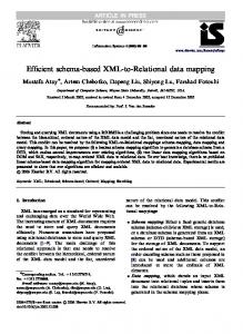
Accurate localisation is arguably the most fundamental competence required by autonomous vehicle systems. It forms the basis for most navigation and control decisions. Without accurate localisation, a mobile robot is essentially left to wander its environment with no notion of where it is and where it is going. While some work, such as the subsumption architecture [7], has suggested that goal-oriented robotic behaviours can be built incrementally with no notion of accurate localisation, most mobile robotic systems require some estimate of their position to perform a desired task. There are many methods by which accurate localisation of a vehicle can be achieved. Some use external sources of information while others rely exclusively on the vehicle’s on-board resources. For many outdoor applications, the deployment of the GPS satellite positioning system has provided a means of estimating the position of a vehicle with high accuracy [47, 46, 61]. Many other applications have used similar external sensors to uniquely determine the position of the vehicle with respect to some coordinate frame. Consider for example acoustic positioning systems prevalent in underwater robotics [43, 52, 67, 70] or external cameras used in some indoor applications. These systems effectively rely on triangulating the position of the vehicle using range and/or bearing measurements to the position of known objects in the environment, as shown in Figure 1.1. External sources of localisation information are not available in all domains and alternate


4

Satellite

Satellite

Satellite

(a) GPS positioning

(b) LBL Positioning

Figure 1.1: Examples of external positioning systems. Both GPS and Long baseline (LBL) positioning systems triangulate the position of the vehicle based on the known positions of the satellites or acoustic transponders. means of localisation have also received a considerable amount of attention. There has been a significant amount of work on map-based localisation and a number of methods have been proposed for achieving accurate localisation given maps of the environment in which the vehicle operates. Beacon based navigation schemes rely on taking observations of beacons whose position in the robot’s environment have been surveyed beforehand [6, 8, 31]. These observations can be fused using an appropriate filter framework, such as the popular Kalman filter, to provide real-time updates of vehicle position with bounded position error . Recent work by Thrun [24, 55, 63] has shown that accurate, robust, real-time localisation can be achieved in indoor environments using grid based and Monte-Carlo methods to estimate the position of a vehicle given a known map of an indoor environment . These applications have typically shown good results in small scale, indoor environments. Similar methods have also been applied to large scale outdoor environments [5]. The literature abounds with other examples of mobile robotic systems that use a variety of sensors, including lasers, sonar and cameras, to perform accurate localisation.

1.2 Problem Summary

1.1.2

5

Mapping

Another important competence for a mobile system is the ability to build and maintain maps of initially unknown environments. Maps allow the vehicle to plan its movement within the environment in order to achieve its goals. The automatic creation of maps allows the vehicle to model the world using its sensory resources. In some instances, the creation of an accurate map of the environment is a goal in itself while in many other circumstances the maps are used as a tool for performing other higher level tasks. Given accurate positioning information, the creation of a map of the environment is a straightforward undertaking. Given a current position estimate and an observation of the environment the observation can be fused into the existing map to create an updated map estimate. Many grid-based approaches have relied on this type of map-building in order to generate an occupancy map of the environment [21, 24, 45]. A number of other mapping techniques rely on the extraction of relevant environmental features with which to build maps [12, 34]. Most feature maps consist of a set of landmarks and encode some relationship between the features contained in the maps. The relationships are often geometrical in nature but, given appropriate sensors, might also encode other properties of the landmarks such as colour, texture or shape. As will be shown in this work, such map building exercises require an accurate, reliable source of localisation in order to guarantee the consistency of the map. In the absence of such information, it will be shown that the only statistically consistent course of action is to maintain an estimate of the correlation between the imperfect estimates of vehicle position and the map.

1.2

Problem Summary

The Simultaneous Localisation and Mapping (SLAM) algorithm provides a means by which a map of the environment can be built while at the same time providing an estimate of the location of the vehicle. By maintaining statistical bounds on the estimated vehicle and observed landmark states, it is possible to quantify the estimated error in the states and

1.3 Principal Contributions

6

to avoid over-confidence in these estimates. As will be shown, one of the fundamental problems with the application of this algorithm is its computational complexity. While it is now possible for the algorithm to operate on larger data sets given recent advances in processor power, there remains a need to manage this complexity effectively. One of the most promising avenues of research into the management of the computational requirements of the algorithm arises from novel methods of representing the information in the map. By manipulating the manner in which information is stored and incorporated into the map, it is possible to reduce the computational burden of updating the map elements.

1.3

Principal Contributions

This thesis addresses the computational issues related to the Simultaneous Localisation and Mapping problem by exploring a number of novel representations for the map. The principal contributions of this thesis arise from the formulation of a new approach to the mapping of terrain features that provides improved computational efficiency in the SLAM algorithm. By manipulating the manner in which feature information is incorporated into the map, it can be shown that significant improvements in the performance of the algorithm can be realised. The contributions made are: • A novel approach to the construction of the SLAM feature map is referred to as the Constrained Local Submap Filter (CLSF). This method generates a local map of the features in the immediate vicinity of the vehicle. This local map is then periodically fused into the global map to recover the full global map estimate. This approach to SLAM is shown to allow a potentially large number of observations to be fused into the global map in a single step, thus increasing the efficiency of the filtering process. Between the application of constraints, only a small, local map must be updated with each observation. Ambiguity in data association is also shown to be reduced by deferring the association of observations to features in the map allowing for a more informed choice of associations. • SLAM using multiple vehicles is shown to be a very natural extension to the CLSF

1.3 Principal Contributions

7

representation and requires only a small modification to the filtering process. Additionally, the multi-vehicle case requires the ability to estimate the relative frames of reference if a vehicle originating from an initially unknown location is to be incorporated into the mapping effort. Methods for establishing this relationship are presented. • The Constrained Relative Submap Filter (CRSF) adopts a similar approach to the CLSF algorithm but maintains the local frames of reference in a tree hierarchy. These independent submaps can then be fused together at some later time to create a consistent global map of the environment. Methods for reinitialising the vehicle in a previous submap and for generating a consistent global map of the environment are both presented in relation to this approach. This approach is shown to improve the computational complexity of the algorithm and can help to address the loop closure problem. • A novel feature initialisation scheme is proposed to improve the performance of the algorithm. In existing implrementations of the SLAM algorithm, features are inserted into the map only after multiple sightings, especially in areas of high signal clutter. The information gathered prior to the confirmation of the feature is discarded to maintain statistical consistency. Rather than discarding observations of tentative features in the environment, this initialisation scheme incorporates them into the filter. When a feature is confirmed through multiple sightings, the information is consolidated into a single estimate of the feature through the application of appropriately formulated constraints. • The thesis also presents results of the application of these techniques to estimate the motion of a vehicle during deployment in an underwater setting. This work represents the first instance of a deployable underwater implementation of the SLAM algorithm. The vehicle model and feature extraction techniques used for generating observations for the filter are outlined. This is followed by results generated from data collected during the deployment of the vehicle in a natural terrain environment. By introducing sonar reflectors into the environment in which the vehicle operated, easily identifiable

1.4 Outline

8

features are made available. These are used to verify the theoretical results developed in this thesis in a practical environment.

1.4

Outline

Chapter 2 presents the Simultaneous Localisation and Mapping algorithms and discusses recent advancements in the field before describing the motivation for the work in this thesis. Chapter 3 presents a novel approach to the map building process - the Constrained Local Submap Filter. This filter relies on building independent local submaps of the features surrounding the vehicle. These submaps are then fused periodically into the global map, allowing the computational burden to be deferred and improving the performance of data association by allowing multiple features to be compared in one hit. Chapter 4 presents a number of related developments that are motivated by the Constrained Local Submap Filter approach to SLAM. These include multi-vehicle SLAM, the Constrained Relative Submap Filter and a novel feature initialisation technique. Chapter 5 presents the application of these techniques to estimate the motion of an Autonomous Underwater Vehicle using a scanning sonar. Finally, Chapter 6 presents conclusions and directions for future research in this exciting field.

Chapter 2

Simultaneous Localisation and Mapping 2.1

Introduction

Simultaneous Localisation and Mapping (SLAM) is the process of concurrently building a feature based map of the environment and using this map to obtain estimates of the location of the vehicle. In essence, the vehicle relies on its ability to extract useful navigation information from the data returned by its sensors. The vehicle typically starts at an unknown location with no a priori knowledge of landmark locations. From relative observations of landmarks, it simultaneously computes an estimate of vehicle location and an estimate of landmark locations. While continuing in motion, the vehicle builds a complete map of landmarks and uses these to provide continuous estimates of the vehicle location. By tracking the relative position between the vehicle and identifiable features in the environment, both the position of the vehicle and the position of the features can be estimated simultaneously. The potential for this type of navigation system for autonomous robotic systems operating in unknown environments is enormous. The SLAM algorithm has recently seen a considerable amount of interest from the mobile robotics community as a tool to enable fully autonomous navigation [10, 18, 23, 32, 50, 53, 62]. This algorithm first appeared in a seminal paper by Smith, Self and Cheeseman [60, 59]

2.1 Introduction

10

that built on previous work by Ayache and Faugeras [2] and Chatila and Laumond [11]. The prospect of deploying a robotic vehicle that can build a map of its environment while simultaneously using that map to localise itself promises to allow these vehicles to operate autonomously for long periods of time in unknown environments. Much of this work has focused on the use of stochastic estimation techniques to build and maintain estimates of vehicle and map feature locations. In particular, the Extended Kalman Filter (EKF) has been proposed as a mechanism by which the information gathered by the vehicle can be consistently fused to yield bounded estimates of vehicle and landmark locations in a recursive fashion [18, 33]. While the Kalman Filter approach to the SLAM problem has received considerable interest, alternative philosophies also appear in the literature. A number of research teams have tackled the problem of map building and localisation using batch estimation techniques [38, 27, 62]. By storing the data collected by the vehicle during its run, they are able to process sensor returns in a batch manner to build maps of the environment in which the vehicle operated. Still other approaches to the problem of map building and localisation have done away with the rigorous mathematical models of the vehicle and sensing properties and have relied instead on more qualitative knowledge of the nature of the environment [7, 30, 36]. These methods have a certain appeal in that they eliminate the need for accurate models of the vehicle motion and sensing processes, limit the computational requirements of map building and have a certain anthropomorphic appeal. While all of these alternative approaches to the problem have their own particular strengths, this thesis will be concerned primarily with a recursive, on-line approach to the problem and will rely on the EKF as the primary means of simultaneously building a map while localising the vehicle. This chapter presents a feature based Simultaneous Localisation and Mapping (SLAM) algorithm used for generating vehicle and landmark feature position estimates based on observations taken relative to the position of the vehicle. Section 2.2 begins by introducing the representation of the state of the vehicle and its environment. Section 2.3 presents the vehicle and landmark models used to describe the vehicle process and landmark observation models commonly employed. Section 2.4 presents a generalised framework for Simultaneous Localisation and Mapping based on an extended Kalman filter. The algorithm consists

2.2 System States

11

of a recursive, three-stage process comprising prediction, observation and update. The mathematical tools necessary to perform each of these steps are presented. Following the development of the algorithm, Section 2.5 discusses a number of issues related to managing the filter before Section 2.6 presents some of the important properties of the algorithm. A number of issues related to computational complexity and maintaining consistency in the estimation process have motivated the development of various novel map representations that have appeared in the literature in recent years. These are reviewed in Section 2.7. This body of work provides the inspiration for the work presented in this thesis and leads to its major contributions. Section 2.8 presents a simulation of the algorithm that serves to highlight its significant characteristics. Finally, Section 2.9 summarises the chapter and provides concluding remarks.

2.2

System States

The SLAM algorithm represents the state of the environment and the state of the vehicle within it as shown in Figure 2.1. The vehicle travels through the environment using its sensors to observe features around it. The state of the system at time k can therefore be represented by the augmented state vector, x(k), consisting of the nv states representing the vehicle, xv (k), and the nf states describing the observed features, xi (k), i = 1, . . . , nf     x(k) =    

Gx

Gx

Gx

where the notation

Gx

i (k)

 v (k) 1 (k) .. .

      

(2.1)

nf (k)

indicates that the state is relative to the frame of reference

FG . Adopting the terminology of Newman [50], the SLAM algorithm in which all states are estimated relative to a common, global frame of reference will be referred to as the Absolute Map Filter (AMF). In the remainder of this chapter, the states are all taken relative to the common, global frame and the reference frame is omitted. This notation will be important in the development in Chapter 3.

2.3 The Vehicle and Landmark Models

12

The system state vector can be written more concisely by lumping the map features into the common term xm (k)

 x(k) = 

Gx

Gx

 v (k)

.

(2.2)

m (k)

Example 2.1. Throughout the remainder of this Chapter, the SLAM equations for a mobile robot navigating in an unknown environment consisting of point features will be developed as an example. This example is intended to illustrate the key steps in the filtering process involved in the SLAM algorithm. Consider the scenario presented in Figure 2.1. The vehicle state at time k can be uniquely determined by its position and orientation in space. The vehicle states are therefore defined by 

 xv (k)

    xv (k) =  yv (k)  .   ψv (k) Each of the point landmark states, xi (k), can by defined by a position in space   xi (k)  xi (k) =  yi (k) and the map vector is defined by 

 x1 (k)    .  xm (k) =  ..  .   xnf (k)

2.3

(2.3)

The Vehicle and Landmark Models

The process model for a system describes how the system states change as a function of time and is usually written as a first order non-linear vector differential equation or state model of the form ˙ x(t) = f (x(t), u(t), t) + v(t)

(2.4)


13

Vehicle Path

zR

Gx

zθ ψv

3 Gx G

FG

1

xv Gx

2

Figure 2.1: The system states involved in the SLAM algorithm. The vehicle travels through the environment taking observations to features using its on-board sensors.


14

where x(t) ∈ Rn is a vector of the states of interest at time t, u(t) ∈ Rr is a known control input, f (·, ·, ·) is a model of the rate of change of system state as a function of time and v(t) is a random vector describing both dynamic driving noise and uncertainties in the state model itself. In general, process models are continuous and must be discretised for implementation on a digital computer. This thesis will consider discrete process and observation models directly but it should be remembered that these models are derived from their continuous time counterparts. The discrete equivalent of equation 2.4 can be written as x(tk ) = f (x(tk−1 ), u(tk ), tk ) + v(tk )

(2.5)

where the function f (·, ·, ·) now maps the state x(tk−1 ) at time tk−1 and the control input u(tk ) at time tk to the state x(tk ) at time tk . In almost all cases considered here, the time interval ∆t(k) tk − tk−1 between successive samples of the state remains constant. In this case, it is common practice to drop the time argument from Equation 2.5 and simply index the variables by the sample number x(k) = f (x(k − 1), u(k)) + v(k)

2.3.1

(2.6)

Vehicle Model

A vehicle model attempts to capture the fundamental relationship between the vehicle’s past state, xv (k − 1), and its current state, xv (k), given a control input, u(k) xv (k) = fv (xv (k − 1), u(k)) + vv (k)

(2.7)

where xv (k) ∈ Rnv are the vehicle states at time step k and vv (k) is a random vector describing both dynamic driving noise and uncertainties in the vehicle state model itself. An accurate vehicle model is an essential component of most navigation schemes. Vehicle models can be of varying degrees of complexity. Depending on the reliability with which the motion of the vehicle can be modeled and the sensors available for predicting the change of


15

state of the vehicle, highly accurate estimates of vehicle motion can be generated. Ideally, of course, a vehicle model would capture the motion of the vehicle without any uncertainty and for each state transition, the vehicle state would be precisely known. This is a practical impossibility, however, as the models used do not, in general, perfectly capture the vehicle motion and sensors and actuators are subject to noise that will slowly corrupt the accuracy of the state estimate. Example 2.2. Returning to the vehicle example considered earlier, a vehicle model for this system describes the motion of the vehicle from one timestep to the next. Assuming that the control inputs at time k are given by the measured wheel velocity, V (k), and steering angle, γ(k), the model for a vehicle of length L is formulated using the common bicycle model, shown in Figure 2.2 [18, 19, 28] 

    xv (k − 1) + ∆t(k)V (k)cos(ψv (k − 1) + γ(k)) vx (k)              yv (k)  = yv (k − 1) + ∆t(k)V (k)sin(ψv (k − 1) + γ(k)) +  vy (k)  .       (k) ψv (k) ψv (k − 1) + ∆t(k)V (k) tan(γ(k)) v ψ L 

xv (k)

2.3.2

Landmark Model

In the context of SLAM, a landmark is a feature of the environment that can be consistently and reliably observed using the vehicle’s sensors. Landmarks must be described in parametric form to allow them to be incorporated into a state model. Point landmarks, corners, line and polyline feature models have all been reported in the literature [9, 32]. For the SLAM algorithm, the feature states are usually assumed to be stationary. While not an essential condition of the SLAM algorithm, tracking moving map features in the environment is not considered of much value for the purposes of navigation. The dynamic portion of the process model therefore consists only of a vehicle model. This leads to the simple landmark model xm (k) = xm (k − 1)

(2.8)

where xm (k)∈ Rnf are the landmark states at time step k. Example 2.3. Given that the position of the landmarks are assumbed to be stationary, the


16

Centre of Rotation

γv

Ψv L Y

(xv,yv) X

Figure 2.2: The simplified bicycle vehicle model. The measured values are the rear wheel velocity, V (k), and steer angle, γv (k). This kinematic model assumes that all points on the vehicle rotate about the Instantaneous Centre of Rotation with the same angular speed. The inputs are used to compute the vehicle position at the following timestep.


17

landmark model for this system is given by xi (k) = xi (k − 1)

2.3.3

(2.9)

Sensor Models

The state observation process can also be modelled in state-space notation by a non-linear vector function in the form z(t) = h(x(t), u(t), t) + w(t)

(2.10)

where z(t) ∈ Rm is the observation made at time t, h(·, ·, ·) is a model of the observation of system states as a function of time and w(t) is a random vector describing both measurement corruption noise and uncertainties in the measurement model itself. These models describe the true observation at time t given the true state of the system x(t). The observation process lends itself well to the discrete observation model z(k) = h(x(k)) + w(k)

(2.11)

as the state observations are often captured using a digital computer system. Example 2.4. The vehicle shown in Figure 2.1 is equipped with a range/bearing sensor that takes observations of the features in the environment. Laser range finders and sonar sensors are two examples of range/bearing sensors that might be used on such a vehicle. Given the current vehicle position xv (k) and the position of an observed feature xi (k), the observation of range, zR (k) and bearing, zθ (k), can be modelled as   zR (k)  z(k) =  zθ (k)     wr (k) (xv (k) − xi (k))2 + (yv (k) − yi (k))2 +  =  (yv (k)−yi (k)) arctan( (xv (k)−xi (k)) ) − ψv (k) wθ (k)

2.4 The Estimation Process

2.4

18

The Estimation Process

Given the process and observation models described in the previous sections, the localisation and map building process consists of generating the best estimate for the system states given the information available to the system. This can be accomplished using a recursive, threestage procedure comprising prediction, observation and update steps known as the Extended Kalman Filter (EKF) [18]. The Kalman filter is a recursive, least squares estimator and ˆ (i|j) of the state x(i) given a produces at time i a minimum mean-squared error estimate x sequence of observations up to time j, Zj = {z(1)...z(j)} ˆ (i|j) = E[x(i)|Zj ] x

(2.12)

The development of the Extended Kalman Filter equations detailed here can be found in numerous texts on the subject [20, 25, 41, 42]. Adopting the notation of Gelb [25], the posterior estimate of the state at time k condiˆ + (k) tioned on the information up to time k will be written as x ˆ + (k) = x ˆ (k|k). x

(2.13)

The prior estimate of the state at time k given the information up to time k −1, also referred ˆ − (k) to as the one-step-ahead prediction, will be written x ˆ − (k) = x ˆ (k|k − 1). x

(2.14)

ˆ − (k) with an observation z(k) of the state x(k) at The filter fuses a prior state estimate x ˆ + (k) (see Figure 2.3). The Kalman Filter makes time k to produce the updated estimate x the simplifying assumption that the process noise, v(k), and observation noise, w(k), are temporally uncorrelated and zero mean E[v(k)] = E[w(k)] = 0, ∀k


19

+

xˆ (k-1), P (k-1)

u(k), U(k)

Process Model

x(k) = f(x(k-1), u(k)) + v(k)

-

xˆ (k), P (k) Observation Model

z(k)=h(x(k)) + w(k)

Data association

z(k), R(k)

Not Matched

z(k) observation of feature i ?

Map management

z(k) a new feature ?

Matched

-

zˆ (k) i

New Feature

+

ν (k), S(k)

Kalman Update

Feature Initialisation

x (k) = x (k) + W(k) ν(k) P+(k) = P-(k) - W(k)S(k)W(k)T

x(k) = g(x(k-1), z(k))

+

-

+

xˆ (k), P (k) Figure 2.3: The essential steps of the filtering process. The state estimate ˆ + (k − 1) and control input u(k) are used to generate a prior state estimate x ˆ − (k). x When observations are received by the filter they are fused to produce the posterior ˆ + (k). estimate x


20

with covariances Q(k)and R(k)respectively E[v(k)vT (k)] = Q(k) E[w(k)wT (k)] = R(k). In some instances, it is also necessary to model inaccuracies in the control input parameters, u(k). These are also modelled as temporally uncorrelated and zero mean E[u(k)] = 0, ∀k with covariances U(k) E[u(k)uT (k)] = U(k).

For the Simultaneous Localisation and Mapping algorithm, the EKF is used to estimate ˆ+ ˆ+ the pose of the vehicle x v (k) along with the positions of the nf observed features x i (k), i = 1...nf . The augmented state vector, Equation 2.1, gives rise to the augmented state estimate consisting of the current vehicle state estimates as well as those associated with the observed features



ˆ+ x v (k)



    + ˆ   x (k) 1 +  ˆ (k) =  .  x   ..    + ˆ nf (k) x

(2.15)

The covariance matrix for this state estimate is defined through ˆ + (k))(x(k) − x ˆ + (k))T |Zk ]. P+ (k) = E[(x(k) − x

(2.16)

This defines the mean squared error and error correlations in each of the state estimates.


21

For the case of the AMF, the covariance matrix takes on the following form 

P+ vv (k)

P+ v1 (k)

. . . P+ vn (k)



    +T + +   (k) P (k) . . . P (k) P v1 11 1n +   P (k) =   .. .. . . . .  . . . .    +T +T + Pvn (k) P1n (k) . . . Pnn (k)

(2.17)

where T k ˆ+ ˆ+ P+ vv (k) = E[(xv (k) − x v (k))(xv (k) − x v (k)) |Z ]

(2.18)

represents the vehicle covariance, T k ˆ+ ˆ+ P+ ii (k) = E[(xi (k) − x i (k))(xi (k) − x i (k)) |Z ], i ∈ {1 . . . n}

(2.19)

represent the landmark covariance, T k ˆ+ ˆ+ P+ v (k))(xi (k) − x vi (k) = E[(xv (k) − x i (k)) |Z ]

(2.20)

represents the cross-covariance between the vehicle and landmark estimate and T k ˆ+ ˆ+ P+ ij (k) = E[(xi (k) − x i (k))(xj (k) − x j (k)) |Z ]

(2.21)

represents the cross-covariance between landmarks. The covariance matrix can be written + more concisely using P+ mm (k) to represent the map covariance and Pvm (k) to represent the

cross-covariance between the vehicle and the map. 

P+ vv (k)

P+ vm (k)



 P+ (k) =  + (k) (k) P P+T vm mm

2.4.1

(2.22)

Prediction

The prediction stage of the filter uses the model of the motion of the vehicle defined in ˆ− Equation 2.7 to generate an estimate of the vehicle position, x v (k), at instant k given the


22

information available to instant k − 1 as ˆ− x x+ v (k) = f (ˆ v (k − 1), u(k)).

(2.23)

The landmark model of Equation 2.8 yields a landmark prediction model as

ˆ+ ˆ− x m (k) = x m (k − 1).

(2.24)

Together, these two models result in the propagation of the augmented state matrix during the prediction cycle of the filter.   f (ˆ x+ (k − 1), u(k)) = v   − ˆ m (k) ˆ+ x x (k − 1) m 

ˆ− x v (k)



(2.25)

The covariance matrix must also be propagated through the vehicle model as part of the prediction. The Extended Kalman Filter linearises the propagation of uncertainty about the ˆ + (k − 1) ˆ + (k − 1) using the the Jacobian ∇x f (k) of f evaluated at x current state estimate x as P− (k) = ∇x f (k)P+ (k − 1)∇x f T (k) + Q(k).

(2.26)

Uncertainty in the control inputs, u(k) used to drive the prediction can be also be accounted for using the control uncertainty, U(k), and the Jacobian ∇u f (k) of f evaluated around the current control inputs P− (k) = ∇v f (k)P+ (k − 1)∇v f T (k) + ∇u f (k)U(k)∇u f T (k) + Q(k). For the SLAM algorithm, this step in the filter can be simplified because of the assumption that the feature states are stationary. This allows the complexity of computing the predicted covariance to be reduced by requiring that only the variances associated with the vehicle and the cross covariance terms between the vehicle and the map are updated during the


23

prediction step 

P− (k)  vv

P−T vm (k)



P− vm (k) 

P− mm (k)

 =

∇ f (k)P+ vv (k  v

− 1)∇v

f T (k)

(∇v f T (k)P+ vm (k

+ Qvv (k)

∇v f (k)P+ vm (k P+ mm (k

− 1)

− 1)

− 1)

 

(2.27) where the noise term, Qvv (k), here represents the lumped process and control noise terms for conciseness. Example 2.5. Considering again the example developed earlier, the prior estimates for the vehicle states at time k given the information available to time k − 1 can be evaluated as   + + ˆ x ˆ (k − 1) + ∆t(k)V (k) cos(ψv (k − 1))  v    −   +  yˆv (k)  =  yˆv (k − 1) + ∆t(k)V (k) sin(ψˆv+ (k − 1))  .     tan(γ(k)) − + ˆ ˆ ψv (k) ψv (k − 1) + ∆t(k)V (k) L 



x ˆ− (k)   v

The propagation of the covariance matrix is accomplished by linearising about the current estimates + T T P− vv (k) = ∇v f (k)Pvv (k − 1)∇v f (k) + ∇u f (k)U(k)∇u f (k) + Q(k)

where

and

  + ˆ 1 0 −∆t(k)Vv sin(ψv (k − 1) + γv )     ∇v f (k) = 1 0 ∆t(k)Vv cos(ψˆv+ (k − 1) + γˆv )    0 0 1 



∆t(k) cos(ψˆv+ (k − 1))

  ∇u f (k) =  ∆t(k) sin(ψˆv+ (k − 1))  ∆t(k) tan(ψˆv+ (k − 1)) ∆t(k) with

 σV2 U(k) =  0

 0 σγ2



0 0 V (k) L cos(ψˆv+ (k−1))2

   

2.4 The Estimation Process   σx2 0 0     Q(k) =  0 σy2 0    0 0 σψ2

and

2.4.2

24

Observation

The fusion of the observation into the state estimate is accomplished by first calculating a ˆ− (k), using the observation model, h as predicted observation, z

ˆ− (k) = h(ˆ x− (k)) z

(2.28)

When observations are received from the vehicle’s on-board sensors they must be associated with particular features in the environment. The difference between the actual observation, ˆ− (k), is termed z(k), received from the system’s sensors and the predicted observation, z the innovation ν(k),

ˆ− (k) ν(k) = z(k) − z

(2.29)

The innovation covariance, S(k), is computed from the current state covariance estimate, P− (k), the Jacobian of the observation model, ∇x h(k), and the covariance of the observation model R(k). S(k) = ∇x h(k)P− (k)∇x hT (k) + R(k)

(2.30)

As will be shown, the innovations and their associated covariances can be used to validate measurements before they are incorporated into the filtered estimates. The calculation of the innovation covariance can be simplified by noting that each observation is only a function of the feature being observed. The Jacobian of the observation function, ∇x h(k), is therefore a sparse matrix of the form ∇x h(k) = ∇v h(k) 0 . . . 0 ∇i h(k) 0 . . . .

(2.31)


25

Evaluating the product in Equation 2.30 using the sparse Jacobian results in − T T S(k) = ∇v h(k)P− vv (k)∇v h (k) + ∇i h(k)Pvi (k)∇v h (k) + − T T ∇v h(k)P−T vi (k)∇i h (k) + ∇i h(k)Pii (k)∇i h (k) + R(k)

(2.32)

Example 2.6. In the application, the vehicle observes the relative range and bearing between ˆ− itself and features in the environment. Given the current vehicle position estimate x v (k) ˆ− and the estimated position of an observed feature x i (k), the predicted observation of range, − (k) and bearing, zˆθ− (k), between the vehicle and the feature can be computed using the zˆR

observation model described in Example 2.4   − (k) z ˆ ˆ− (k) =  R  z zˆθ− (k)  

− − − 2 + (ˆ 2 (ˆ x− (k) − x ˆ (k)) y (k) − y ˆ (k)) v v i i  =  (ˆ yv− (k)−ˆ yi− (k)) − ˆ arctan( (ˆx− (k)−ˆx− (k)) ) − ψv (k) v

i

To find the innovation covariance, the Jacobians of the observation equation, h, with respect to the vehicle states, ∇v h(k), and with respect to the feature states, ∇i h(k) must be ˆ − (k) results in computed. Evaluating the Jacobian at the prediction x  ∇v h(k) =

x ˆ− x− v (k)−ˆ i (k) d  − yˆ (k)−ˆ y − (k) − v d2 i

 − x ˆ (k)−ˆ x− (k) − v d i ∇i h(k) =  − − yi (k) yˆv (k)−ˆ d2

with d=

yˆv− (k)−ˆ yi− (k) d x ˆ− x− x (k)−ˆ i (k) d2

 0 −1 



yˆv− (k)−ˆ yi− (k) d  x ˆ− x− v (k)−ˆ i (k) − d2

−

2 ˆ− yv− (k) − yî− (k))2 (ˆ x− v (k) − x i (k)) + (ˆ

Section 2.5.2 will describe how the innovation and its covariance can be used for the purposes of data association.


2.4.3

26

Update

Once the observation has been associated with a particular feature in the map, the state estimate can be updated using the optimal gain matrix W(k). This gain matrix provides a weighted sum of the prediction and observation and is computed using the innovation covariance, S(k) and the predicted state covariance, P− (k). The weighting factor is proportional to P− (k) and inversely proportional to the innovation covariance [60]. This is used ˆ + (k) as well as the updated state covariance P+ (k). to compute the state update x ˆ − (k) + W(k)ν(k) ˆ + (k) = x x

(2.33)

P+ (k) = P− (k) − W(k)S(k)WT (k)

(2.34)

W(k) = P− (k)∇x hT (k)S−1 (k)

(2.35)

where

2.4.4

Feature Initialisation

When a new feature is observed its estimate must be properly initialised and added to the ˆ− ˆ − (k), comprised of the vehicle state, x state vector. Given a current state estimate, x v (k), ˆ− and the map states, x m (k), a relative observation between the vehicle and the new feature, z(k), and a feature initialisation model, gi (·, ·), that maps the current vehicle state estimate and observation to a new feature estimate, the initial estimate of the feature state is ˆ+ x− x v (k), z(k)). i (k) = gi (ˆ

(2.36)

These new state estimates are then appended to the state vector as new map feature elements. The covariances of the new feature estimates must also be properly initialised since the initial estimate depends on the current vehicle estimate and is therefore correlated with the rest of the vehicle and other map state estimates. Ignoring the correlation between the new state estimates and the remainder of the map can lead to inconsistency in the filtering process [14]. The AMF covariance matrix is first augmented with the observation


27

covariance and the cross-covariance terms between the existing state elements and the new state estimates are computed. Assume the initial covariance matrix, P− (k), is 

P− vv (k)

P− vm (k)



 P− (k) =  − (k) (k) P P−T vm mm

(2.37)

The covariance matrix is then augmented with the observation covariance, R(k)  P∗− (k)

P− (k)  vv



P− vm (k)

0    −T = Pvm (k) P− 0  mm (k)   0 0 R(k)

(2.38)

The final covariance is computed by projecting the augmented covariance matrix through the Jacobian ∇x g(k) of the initialisation function, gi , with respect to the augmented states,

P+ (k) = ∇x g(k)P∗− (k)∇x gT (k) 



with

(2.39)

Iv

0

0

    ∇x g(k) =  0 0 . Im   ∇v g(k) 0 ∇z g(k)

(2.40)

This O(n3 ) operation can be simplified by exploiting the sparse nature of the Jacobian, ∇x g(k) 

P− vv (k)

P− vm (k)

T (P−T vv (k)∇v g (k))



    − (k) −T (k)∇ gT (k)) P+ (k) =  P−T  (k) P (P v vm mm vm   − (k) ∇ g(k)P− (k)∇ gT (k) + ∇ g(k)R(k)∇ gT (k) (k) ∇ g(k)P ∇v g(k)P− v v v z z vv vm vv (2.41) Proper initialisation of the feature estimates is necessary to maintain their consistency and to generate the correct cross-covariances between the feature and vehicle estimates. Example 2.7. In order to complete the example application developed in the previous Sections, the initialisation equations for adding a new feature into the map are shown here.

2.5 Filter Management

28

ˆ− Given a current vehicle estimate x v (k) and an observation z(k) of a feature i that does not ˆ+ yet exist in the map, the initial estimate, x i (k), of the location of the feature is computed using the non-linear initialisation function gi     − (k) + z (k) cos(ψ ˆ− (k) + zθ (k)) (k) x ˆ+ x ˆ R v  i = v  + − − ˆ yî (k) yˆv (k) + zR (k) sin(ψv (k) + zθ (k)) Given this initialisation equation, the required Jacobians with respect to the vehicle states, ∇v g(k), and the observation, ∇z g(k) can be evaluated at the current estimate as   − ˆ 1 0 −zR (k) sin(ψv (k) + zθ (k))  ∇v g(k) =  − ˆ 0 1 zR (k) cos(ψv (k) + zθ (k))   cos(ψˆv− (k) + zθ (k)) −zR (k) sin(ψˆv− (k) + zθ (k)) . ∇z g(k) =  − − ˆ ˆ sin(ψv (k) + zθ (k)) zR (k) cos(ψv (k) + zθ (k))

2.5

Filter Management

To successfully manage the estimation process, and to supply it with reliable and robust feature observations, a number of additional considerations must be taken into account. These include the methods used for extracting and identifying features and for data association when new observations are received. This section examines some of these issues in more detail.

2.5.1

Feature Extraction

The development of autonomous feature based navigation relies on the ability of a sensor system to extract appropriate and reliable features with which to build maps. The feature extraction process is highly application dependent and depends on the anticipated environment in which the vehicle will operate, and the sensors used to observe this environment. Some environments, such as those found in typical offices, lend themselves to the extraction of corner and line features using such sensors as lasers and vision systems. In unstructured


29

environments, simple corner or line features are not commonly observed. Additionally outdoor sensors very often can not provide the same accuracy or detail as can be obtained from indoor navigation sensors. Should the vehicle be required to operate in more unstructured environments, these features may prove to be insufficient for modelling the vehicle’s surroundings. Alternative methods for terrain modelling have recently appeared in the literature [39] and it will be interesting to see how some of this work develops over the coming years. This thesis will concern itself primarily with SLAM using point features. Point features are simply defined as a point in the environment that yields consistent, reliable and viewpoint invariant sensor returns. What constitutes a good point feature will once again be application dependent, and in particular will be affected by the quality of available sensors. However, the techniques presented are not limited to the estimation of point features. They can readily be extended to include the estimation of any alternative feature types that can be parametrised for use in the Kalman filter framework.

2.5.2

Data Association

Data association is the process matching observations that are received by the filter to the features to which they correspond. Given that the state estimation process relies on generating statistical estimates of the locations of features in the environment, statistical methods are used for establishing these associations. The most common method for associating observations to features in the map relies on nearest neighbour techniques [18, 22, 35, 50]. A Nearest Neighbour association is taken in this case to be the closest association in a statistical sense. A common statistical discriminator is based on the normalised innovation squared between two estimates. Given an observation z(k) comprising a range and bearing to the observed landmark, the innovation, ν(k), and innovation covariance, S(k), can be calculated as shown in equations 2.29 and 2.30 respectively. The normalised innovation squared between the observation and the estimated feature location is then compared against a validation gate, dmin , for the association being considered. df i = ν T (k)S−1 (k)ν(k) < dmin

(2.42)


30

The normalised innovation squared forms a χ2 distribution that can be used to accept or reject a particular association with a given confidence level by the appropriate selection of dmin . Data association is essential to the operation of the Simultaneous Localisation and Mapping algorithm. The estimated location of landmark positions rely on the accuracy of the vehicle location estimate. An incorrect association of an observation to the map can cause the filter to diverge from a consistent estimate, effectively rendering all future predicted observations incorrect. Unfortunately, it is quite difficult to detect and recover from an incorrect association by relying exclusively on nearest neighbour techniques as associations depend on calculating a predicted observation based on the current estimate of vehicle location. If the vehicle location estimate is in error, then an observation to a known landmark will be estimated to have occurred from a different map position. In this case, there is a risk that the filter may incorrectly associate the observation with another landmark in the map or initialise a new feature at this position. Recent work in this area has examined the possibility of using multiple hypothesis approaches [57] or joint compatibility criteria [48] to improve the performance of data association when compared with simple nearest neighbour approaches. Chapter 3 presents a novel approach to the SLAM algorithm that can help to address this issue. As will be shown, using multiple features for generating associations can serve to increase the probability of correct associations by decreasing the number of plausible vehicle positions that might have produced the observations in question. Increasing the number of features available for matching is shown to increase the probability of yielding a correct match between feature sets.

2.5.3

Map Management

Once features have been identified, they must be matched against known landmarks in the environment. The first step is to perform data association between the observed feature and the features currently in the map. This step is one of the most crucial in the mapping


31

process. Erroneous data association can destroy the integrity of the map. When data is received from a sensor there is a possibility that it may in fact be a spurious measurement. Some spurious measurements can be eliminated by the development of appropriate feature extraction routines: by studying and modeling the physical phenomena that are being measured by the sensor it is possible to reduce the number of spurious measurements picked up by a feature extractor. Regardless of the care that is taken in designing the feature extractor, some spurious measurements may still be passed to the localisation and mapping algorithm and it is important to have a mechanism for rejecting these. A two-step matching algorithm is used in order to reduce the number of landmarks that are added to the map (see Figure 2.4). When a new range and bearing observation is received from the feature extraction process, the estimated position of the feature is computed using the current estimate of vehicle position. This position is then compared with the estimated positions of the features in the map using the data association strategies given in Equation 2.42 [18]. If the observation can be associated to a single feature the EKF is used to generate a new state estimate. An observation that can be associated with multiple landmarks is rejected since false associations can destroy the integrity of the estimation process. If the observation does not match to any landmarks in the current map, it is compared against a list of tentative landmarks. Each tentative landmark maintains a counter indicating the number of associations that have been made with the feature as well as the last observed position of the feature. If a match is made, the counter is incremented and the observed position is updated. When the counter passes a threshold value, the feature is considered to be sufficiently stable and is added to the map. If the potential feature cannot be associated with any of the tentative features, a new tentative feature is added to the list. Tentative features that are not reobserved are removed from the list after a fixed time interval has elapsed.


32

New Range/ Bearing to feature received

Match to feature in the map?

No

Match to tentative feature list?

Yes

Yes

Update position and increment match count Match multiple features in map?

Yes

No

Pass Range Bearing observation to filter along with matched feature index

Is Count > threshold?

Yes

Reject multiple feature matches to avoid corrupting the map

Add a new feature to the map and remove the current tentative feature from the list.

Figure 2.4: The feature matching algorithm

No

Add a new tentative feature to the list

2.6 Properties of the SLAM Algorithm

2.6

33

Properties of the SLAM Algorithm

The SLAM algorithm has a number of important properties that regulate the growth of uncertainty in both the map and vehicle estimates. These properties include the convergence of the map state estimates, the need to maintain consistency in the estimation process and the computational complexity involved in maintaining the AMF state covariance matrix. This section examines some of these issues in more detail and provides references for related work that appears in the literature.

2.6.1

Convergence

In his thesis [50], Newman was first to prove three important convergence properties of the SLAM filter. These results built on work by Csorba [14] and appear in [18]. The three key results can be summarised as follows.

1. The determinant of any submatrix of the map covariance matrix decreases monotonically with every observation made. 2. In the limit, as the number of observations increases, the landmark estimates become fully correlated. 3. The lower limit of map accuracy is a function of initial vehicle uncertainty when the first landmark is observed.

These properties of the SLAM algorithm have important implications for its application to real world systems. The proofs effectively demonstrate that the uncertainty in the map estimates will tend to decrease to some lower bound and that the relationships between features or landmarks will become perfectly known. Given particular vehicle and sensor models and some notion of the estimated feature density in the environment, it is possible to predict the filter’s steady state performance. This allows the expected long term performance of the algorithm to be specified as a function of the accuracy of the sensors and vehicle models being used.


2.6.2

34

Maintaining Consistency in SLAM

In order to maintain the consistency of the estimate generated by the SLAM algorithm, it is necessary to update the AMF covariance matrix with each observation using Equation 2.34. Csorba has demonstrated that this is essential to avoid inconsistency in the estimation process [14]. Since observations of the terrain features are taken relative to the vehicle, any error in the vehicle estimate will be strongly correlated with errors in the map estimates. Figure 2.5 shows the effect of an error in the initial estimate of the vehicle position on the accuracy of the rest of the map. Since all observations are made relative to the estimated position of the vehicle, this initial error will be propagated to the estimates of the positions of all the features. In his thesis [14], Csorba showed that there will be a common uncertainty in the map estimates associated with the initial uncertainty when the first feature is observed. Without external information regarding the positions of the landmarks or the vehicle, it is essential that the correlation between the states be maintained in order to maintain consistent error bounds on the estimated states. This need to maintain the all of the covariances between the vehicle estimate and all the elements in the map is the source of the computational complexity inherent in the SLAM algorithm.

2.6.3

Computational Complexity

One significant obstacle on the road to the implementation and deployment of large scale SLAM algorithms is the computational effort required to maintain the correlation information between features in the map and between the features and the vehicle. Performing the update of the covariance matrix is of O(n3 ) for a straightforward implementation of the Kalman Filter. In the case of the SLAM algorithm, this complexity can be reduced to O(n2 ) given the sparse nature of typical observations. Even so, this implies that the computational effort will grow with the square of the number of features maintained in the map. For maps containing more than a few tens of features, this computational burden will quickly make the update intractable - especially if the observation rates are high. An effective map-management technique is therefore required in order to help manage this complexity.


35

Vehicle Path

zi zi 0x 3

F0

0x 3 0

xv

F0

0x 1

0x 1

0x v 0x 2

0x 2

Figure 2.5: The effect of vehicle-map correlation. The darker elements represent the estimated positions of the vehicle and landmarks while the lighter elements show the true positions. Clearly, the error in the vehicle estimate has been reflected in an error in the landmark estimates.

2.7 Managing Complexity

2.7

36

Managing Complexity

A number of potential methods by which the growth of the computational burden imposed by the covariance update can be regulated have been described in the literature. This section examines a number of these methods, touching on their major strengths and weaknesses. Many of these approaches have been motivated by the search for an efficient method for maintaining consistent estimates of the map states without performing a complete update of the covariance matrix with each observation. The traditional SLAM algorithm requires such an update and it is well known that this step makes the filter difficult to implement in real-time for large maps. A number of approaches to the SLAM problem that improve the computational complexity of the update step are reviewed and the salient features of each method are presented. These can be divided into three broad categories. Some work has concentrated on the reduction in complexity that can be achieved by concentrating on fewer features or even eliminating features. Results suggest that the computational burden can be reduced without significant loss of information. Other work has examined the possibility of applying suboptimal update steps to once again reduce the complexity of updating the state covariance matrix. Finally, a number of researchers have proposed alternative map representations that change the manner in which information is added to the maps.

2.7.1

Limiting the Number of Features

One method for improving the algorithm’s performance is to limit the number of features that are included in the map. Active sensing, in which a sensor is controlled to look at only a limited part of the environment, is one way of limiting the number of features to be considered for inclusion in the map. To use active sensing effectively features that are likely to remain visible during the vehicle’s motion must be identified. An effective metric for the value of new landmarks may therefore come from the geometric distribution of landmarks as a function of the current vehicle trajectory. In Davison’s thesis [16] it is shown that active sensing can be performed to concentrate on a few, reliable features using a vision sensor mounted on an active pan tilt head. Accurate SLAM is shown to be possible despite


37

the fact that not all of the considerable information contained in the visual images is used. Alternatively, features can be deleted from the map after the vehicle has left an area to once again limit the growth of the size of the map [17]. A suitable cost metric could be used to evaluate the loss of information resulting from the removal of a feature. As might be expected, this loss of information will lead to a sub-optimal estimate. However, the amount of information loss may be acceptable and will be offset by the computational savings achievable. Suitable metrics for the selection of features to be removed from the state matrix may therefore come from the amount of information contained in the estimate of a feature [17]. The geometric distribution of landmarks may also play a role in the selection process. Once the vehicle reenters an area it has previously explored, it may not see the limited features that it has remembered and the uncertainty in vehicle position will not be reduced despite the fact that the vehicle is operating in an area it has previously explored.

2.7.2

Sub-optimal Updates

As an alternative to limiting the number of features in a map, the use of sub-optimal or nearoptimal covariance updating schemes has also been considered. Conservative covariance update techniques can be shown to improve the computational performance of a SLAM algorithm at the expense of some loss of information.

Covariance Intersect Uhlmann et al have proposed a conservative algorithm for combining state estimates and computing an updated covariance matrix without a priori knowledge of the correlations between states. This approach substantially decreases the computational complexity of the SLAM problem using the covariance intersect (CI) method [65]. The CI method does not require knowledge of the cross-correlations between states and only the diagonal elements of the state covariance matrix need to be maintained. Each observation is conservatively fused into the estimated state matrix through the use of the covariance intersect algorithm. Given


38

− − two mean and covariance estimates, {ˆ x− x− a (k), PAA (k)} and {ˆ b (k), PBB (k)}, the covariance + intersect update, {ˆ x+ c (k), PCC (k)}, is computed as

− − −1 P+ CC (k) = (ωPAA (k) + (1 − ω)PBB (k)) + − − ˆ+ x x− x− c (k) = PCC (k)(ωPAA (k)ˆ a (k) + (1 − ω)PBB (k)ˆ b (k))

(2.43) (2.44)

where 0 ≤ ω ≤ 1 and ω can be computed to minimise any chosen measure (e.g. determinant, trace, maximum eigenvalue, etc.) of the updated covariance matrix. The proof that this algorithm is conservative is shown in [65, 66]. For the case of the SLAM problem, the prior − estimate of the feature location is chosen as estimate {ˆ x− a (k), PAA (k)} and the observation − as estimate {ˆ x− b (k), PBB (k)}.

This approach provides a computationally efficient mechanism for performing SLAM but discards a considerable amount of information contained in the covariance between the feature state estimates. This information usually allows improvements in the vehicle and map estimates to be be propagated throughout the map when a well-known feature is observed and is the key to the convergence properties of the algorithm. As shown in [65], feature estimates taken far from the vehicle’s initial position have large covariances which are not much improved when the vehicle returns to its initial position. This large covariance can make data association difficult and may not allow the map estimates to converge.

Partitioned Update Guivant et al [26] have recently proposed a simplification to the update step of the SLAM filter that can significantly reduce its computational complexity. Their main insight comes from the fact that the update of a large proportion of the features in the map is insignificant. This fact leads them to update only a select subset of the map features during a particular observation, reducing the computational burden to O(n), where n is the number of states in the map. This results in a significant improvement in computational effort for large maps.


39

The state matrix can be partitioned, without loss of generality, such that  ˆ − (k) = x



ˆ − (k) x  A  ˆ− x B (k)



RnA



 , n = nA + nB ∈ n B R

(2.45)

The state covariance matrix after an optimal update can now be written as 

P+ (k)  AA



P+ AB (k)

+ P+T AB (k) PBB (k)

 =

P− (k)  AA



P− AB (k)

− P−T AB (k) PBB (k)

 −

∆P− AA (k) 



∆P− AB (k)

− ∆P−T AB (k) ∆PBB (k)

.

(2.46)

A conservative covariance update is sought that minimises the loss of information during the update. This in turn leads to the following conservative covariance update 

− P− AA (k) PAB (k)





− ∆P− AA (k) ∆PAB (k)

− P∗+ (k) =  − (k) P (k) P−T ∆P−T AB BB AB (k)

 

(2.47)

0

or P∗+ (k) = P− (k) − ∆P∗− (k)

(2.48)

that is shown to be consistent. The new update term, ∆P∗− (k), requires the calculation of − the nA ×nA upper block matrix ∆P− AA (k) plus the nA ×nB cross-covariance term ∆PAB (k).

This calculation will require a multiplication of O(nA 2 ) plus a mutliplication of O(n). If the state matrix for the SLAM algorithm is partioned such that nA n this update term will therefore be of O(n) for large n. The partitioning of the state matrix required for the conservative update mechanism will determine the degree to which the update is conservative. In the case of the SLAM ˆ− algorithm, the partitioned states, x B (k), are chosen from the feature estimates currently contained in the map. The feature states chosen for the partitioned states will not have their covariance estimate updated during an observation. The cross-covariance terms with ˆ− the x A (k) states must be calculated to maintain the consistency of the covariance estimate. One of the properties of the SLAM algorithm is that the estimated covariance of the landmark states will decrease monotonically to some lower bound [18]. Each update will contribute some information to the state estimate of all the features in the map. The amount


40

of information contributed to each feature estimate will depend on its current covariance ˆ− estimate as well as its correlation with the other features in the map. The choice of x B (k) is made prior to each update to minimise the loss of information from a suboptimal update. Guivant et al [26] propose two mechanisms for partitioning the update matrix based on the relative change in the covariance estimate for each state and the absolute value of the covariance estimate.

2.7.3

Alternative Map Representations

Much work in recent years has concentrated on the effect of the map representation on both the computational complexity of the SLAM algorithm and on the achievable estimation accuracy. In this section, a number of alternative map representations will be described. The significant characteristics of each of these representations will be discussed.

Relative Maps In his thesis, Csorba proposed using the relative position between features rather than their absolute position as state variables [14] [15]. The relative location between landmarks is clearly independent of any absolute coordinate frame and of the location of the vehicle during an observation. Consequently, relative location estimates are uncorrelated. The covariance matrix is therefore diagonal and each observation can be fused into the filter by only updating the estimate of the relative state being observed. Newman developed this idea further and showed that while the relative representation is computationally efficient, it can result in inconsistent estimates of the relative states [50]. For example, given estimates of the relative position between three landmarks, these independent estimates may not be mutually consistent. Newman proposed the Geometric Projection Filter (GPF) as a mechanism with which to enforce the consistency of the relative state estimates. By applying constraints to the relative states, Newman was able to recover a consistent map estimate at appropriate intervals at the cost of introducing correlations between the states. It was suggested that the relative state estimates be maintained in one filter and that at appropriate intervals the constraints be applied to recover a consistent


41

map. This consistent map could then be used for reasoning about the state of the map. New observations were fused into the original, relative map as they were received by the filter and the process of applying the constraints repeated at appropriate intervals to recover the consistent map. Newman also pointed out a number of difficulties that may arise from the relative representation of the map states. In particular, data association is potentially very difficult using a relative state representation. Consider a hypothetical scenario in which the vehicle moves amongst equally spaced features. Matching a relative observation to a particular state is impossible without some knowledge of the absolute location of the vehicle and feature states. This requirement counteracts the computational savings that can be realised using the relative representation of the map by requiring that the map be transformed to the absolute frame of reference for the purposes of data association. While this situation is an extreme example, it serves to illustrate the potential data association problems that may arise through the use of the relative filter. In addition, Newman’s GPF does not maintain an estimate of the vehicle position. While this information can be estimated using observations of particular features in the environment, it is subject to errors arising from false associations and/or spurious measurements.

Submaps Another possibility is to divide a large map into a series of smaller submaps in order to reduce the computational complexity of the covariance update step. This approach has been adopted by a number of researchers. Chong and Kleeman [13] have proposed a submap strategy whereby a number of independent, local submaps are generated as the vehicle operates. Estimates of the relative position between the submaps are maintained and a search algorithm is instantiated to relocalise the vehicle when the vehicle estimate has a high likelihood of being in the area of a previous local submap. This hierarchical approach to the mapping problem is shown to drastically reduce the memory and processing time requirements when compared with the global approach to SLAM.


42

Chong and Kleeman do not provide methods for generating a globally consistent map of the environment. They suggest that this might be a possible extension to their work and might be accomplished using a least squares formulation. In this work it will be shown, through the development of the Constrained Relative Submap Filter in Chapter 4, that globally consistent maps of the environment can in fact be generated through the use of appropriately formulated constraints. A computationally efficient method for SLAM using a number of globally referenced submaps is presented by and Leonard and Feder [22, 35]. In this scheme, the submaps are allocated in an a priori manner and a unique vehicle state is associated with each submap. Methods are presented for transitioning the vehicle state estimates from one submap to another in a conservative manner. The method presented by Feder and Leonard has been demonstrated to yield empirically consistent mapping results with significant improvements in computational complexity. It relies, however, on a number of assumptions about the propagation of error between the vehicle and map states. The method they describe for performing cross-map vehicle relocation relies on randomizing the current vehicle estimate within the confines of the submap being considered and using the prior vehicle estimate from the previous submap as an observation of vehicle position. This approach is shown to yield acceptable results in practice, however it can be shown to be inconsistent in the manner in which the vehicle estimate is reinitialised. In theory, the initial vehicle uncertainty when re-entering a submap should be infinite prior to its initialisation - in a similar manner to that used for initialising map feature estimates. A more consistent method for transitioning the vehicle would be to reinitialise the vehicle state based purely on observations of the features in the submap. This approach will feature in the development of the work in this thesis. Finally, recent work by Castellanos et al has introduced another method of performing SLAM [10] using global and local frames of reference in the mapping process. Feature sets are estimated with respect to landmark frames, themselves estimated in the global frame of reference. Constraints between the various frames of reference are then used to generate a consistent global estimate of the vehicle state. A unique vehicle estimate is maintained with respect to each of the landmark frames. These distinct vehicle estimates are then fused

2.8 Simulation

43

together, using constraints, to recover a consistent estimate of the map states. One problem with the approach proposed by Castellanos et al arises during the propagation of the various vehicle state estimates. The vehicle models employed are often characterised by a large growth in uncertainty during the prediction step. The SLAM process allows this growth of uncertainty to be regulated through the use of terrain information which acts to slow uncertainty growth. Given that the independent vehicle estimates rely exclusively on dead reckoning when the vehicle is not observing features in its frame of reference, the covariances associated with the independent vehicle estimates will grow large. When constraints are applied, there is a risk that non-linearities introduced by large covariances and large estimation errors may affect the achievable estimation accuracy.

2.8

Simulation

This section presents results of the application of the SLAM algorithm using a simulated environment. The vehicle and feature observation models developed by the examples presented in the previous sections are used. Simulation is useful for understanding and verifying the performance of the algorithm as the true vehicle and feature locations are available. This allows for comparison between the true state of the system and the estimates generated by the filter. During the deployment of a vehicle in a field environment, ground truth is often not available and it is more difficult to accurately verify the performance of the algorithm. Figure 2.6 shows a map of a simulated environment in which the vehicle described in the example is operating. As can be seen, the desired vehicle trajectory is approximately circular. The landmarks are randomly distributed throughout the environment and the vehicle takes noisy range/bearing observations to random features that fall within the range of it’s on-board sensor. The filter parameters used for the simulation are shown in Table 2.1. This same simulator will be used throughout the remainder of the thesis to illustrate key properties of the algorithms developed. Figure 2.7 shows the error in the estimate of the vehicle location along with the ±2σ confidence bounds. The global vehicle covariance grows large as the vehicle navigates around the loop. As the vehicle approaches its initial location, a large correction in the estimate

2.8 Simulation

44

100

80

60

40

20

0

0

20

40

60

80

100

Figure 2.6: The simulation environment showing the desired vehicle trajectory and the landmarks randomly scattered through the environment.

Table 2.1: Simulation filter parameters Sampling period ∆t(k) 0.1s Vehicle velocity std dev σv 0.05V (k)m/s Vehicle steer angle std dev σγ 0.005rad Range measurement std dev σR 1.0m Bearing measurement std dev σB 0.05rad Vehicle Length L 1.5m Sensor range 25m

2.8 Simulation

45

X error (m)

4 2 0 −2 −4

0

100

200

300

400

500 time (s)

600

700

800

900

1000

0

100

200

300

400

500 time (s)

600

700

800

900

1000

0

100

200

300

400

500 time (s)

600

700

800

900

1000

Y error (m)

5

0

−5

Psi error (rad)

0.04 0.02 0 −0.02 −0.04

Figure 2.7: Errors in the vehicle state estimates together with the estimated 2σ covariance bounds. The AMF covariance estimates are shown for the vehicle pose states (xv , yv , ψv ). The errors appear to be within the 95% confidence bounds defined by the 2σ gate showing that the filter is well tuned. and corresponding reduction in position uncertainty occurs just before 300s as the vehicle observes a feature with low variance. The errors in the vehicle estimates are within the 2σ covariance bounds most of the time showing that the filter is well tuned. The innovation sequences can also be checked to verify that the observation sequences are bounded. This is clearly the case as shown in Figure 2.8. Given that the true state models are known in simulation, generating a well tuned filter is straight forward. For real systems, the models must often be tuned through an experimental process in order to work correctly, although careful modeling of sensors and the environment can help to produce a well matched filter. One of the major concerns with the SLAM algorithm is the computational complexity of the covariance update step. Figure 2.9 shows the floating point operations required by the

2.8 Simulation

46

Range Innovation (m)

3 2 1 0 −1 −2 −3

0

100

200

300

400

500 time (s)

600

700

800

900

1000

0

100

200

300

400

500 time (s)

600

700

800

900

1000

Bearing Innovation (rad)

2

1

0

−1

−2

Figure 2.8: The innovation sequences. The estimates appear to be zero-mean and white with approximately 95% of the innovations falling within the 2σ innovation covariances bounds, again demonstrating that the filter is well tuned.

2.8 Simulation

47

M Floating Point Operations 0.25

0.2

M Flops

0.15

0.1

0.05

0

0

100

200

300

400

500 Time (s)

600

700

800

900

1000

800

900

1000

(a) Floating Point Operations

Cumulative M Floating Point Operations 2000

1800

1600

1400

M Flops

1200

1000

800

600

400

200

0

0

100

200

300

400

500 Time (s)

600

700

(b) Cumulative Floating Point Operations

Figure 2.9: The floating point operations required for the prediction and update stages of the filters. The spikes in the plot occur when new features are initialised or observations are rejected by the innovation gates. These operations require significantly less floating point operations than an update of the covariance matrix.

2.8 Simulation

48

Beacon Positions

Beacon Positions 18

100

16 14

80

10

60 Y (m)

Y (m)

12

8 6

40

4 2

20

0

0

−2

0

20

40

60 X (m)

80

100

5

(a) The final AMF map

10

15 X (m)

20

25

(b) An enlarged portion of the map near the origin

Beacon Positions 50

Beacon Positions 110

45 105

100

Y (m)

Y (m)

40

95

35

90

30 85

25 85

90

95 X (m)

100

105

(c) An enlarged portion of the map on the outward leg

50

55

60

65

70

75

X (m)

(d) An enlarged portion of the map as it returns

Figure 2.10: The final map estimates. As can be seen from the close-up portions of the map, the map estimates (+) and their associated covariance bounds are clearly consistent with the true feature locations (o).

2.9 Summary

49

algorithm to maintain the estimates. The computational burden rises quadratically until all of the observable features have been incorporated into the map. The complexity of each update is then maintained. The cumulative floating point operations are linear once all the features have been incorporated into the map. The maps generated by the algorithm can be examined to verify that the algorithm does, in fact, yield a consistent map. Figure 2.10 shows the map generated by the algorithm along with the actual position of the landmarks. This map is consistent with the true location of the features. It is interesting to note that features that are far from the origin maintain a higher covariance bound than those incorporated early in the run. The uncertainty that results from the application of the vehicle model accounts for this effect.

2.9

Summary

This chapter has reviewed the current state of the art of the Simultaneous Localisation and Mapping algorithm. The three step estimation process involving prediction, observation and update of the estimated states using the Extended Kalman Filter formulation were described. This was followed by a discussion of feature management techniques required for data association, feature identification and initialisation. Motivation for the work in the remainder of this thesis was also presented. Given the computational complexity inherent in the update step required to maintain consistent maps, there has been a considerable amount of work in recent years examining alternative map representations that can help to minimise the cost of an update. This work is reviewed and the major contributions of each approach are examined. While there have been some major developments in this field in recent years regarding the performance of this algorithm, there is still a need for further improvements before a long duration, real time version of the SLAM algorithm can be deployed. This thesis presents a novel approach the construction of the feature map that helps to further manage the complexity of the update. In spite of its weaknesses in the area of data association, the relative map representation presented by Csorba and later adopted by Newman for the GPF is characterised by a number of appealing characteristics in terms of

2.9 Summary

50

computational complexity. These characteristics motivate the development of an approach to the construction of the SLAM map that forms the major contribution of this thesis. This method forms the basis of chapter 3 and extensions to the method are presented in Chapter 4.

Chapter 3

The Constrained Local Submap Filter 3.1

Introduction

This chapter presents a novel approach to SLAM that exploits the manner in which observations are fused into the global map of the environment to manage the computational complexity of the algorithm and improve the data association process. Rather than incorporating every observation directly into the global map of the environment, the Constrained Local Submap Filter (CLSF) creates an independent, local submap using observations of the features present in the immediate vicinity of the vehicle. This local submap is then periodically fused into the global map of the environment. It will be shown that this approach to the SLAM algorithm reduces the computational complexity of maintaining the global map estimates and improves the data association process. Section 3.2 begins by summarising the key characteristics of the proposed SLAM algorithm. Section 3.3 describes the system states that are estimated. Section 3.4 describes the estimation process using this representation and highlights the differences between it and the AMF. Section 3.5 demonstrates that the local vehicle and map feature estimates are, in fact, independent of the global map feature estimates. Section 3.6 describes the mechanism used to transform the local states estimates into the global frame of reference. Section 3.7

3.2 Constrained Local Submap Filter

52

introduces a mechanism for fusing the local map into the global map through the application of appropriately formulated constraints in order to recover all of the information gathered by the sensors. Section 3.8 describes the computational savings that are realised with this approach and Section 3.9 discusses methods that can be used for establishing data association between the feature estimates. Section 3.10 presents simulation results illustrating the application of the approach, highlighting the performance of the Constrained Local Submap Filter. Finally, Section 3.11 summarises the chapter and provides concluding remarks.

3.2

Constrained Local Submap Filter

The Constrained Local Submap Filter (CLSF) presents a novel scheme for addressing the computational complexity of the SLAM algorithm by allowing the update of the full covariance matrix to be scheduled at appropriate intervals. The method developed here maintains an independent, local submap estimate of the features in the immediate vicinity of the vehicle (see Figure 3.1). The observations are fused into an independent submap centered at a local frame of reference whose global position is known. At appropriate intervals, the information contained in the local map is transferred into the global map and a new local map is created. It will be shown that, subject to the usual linearising assumptions, the resulting map and vehicle estimates are identical to those obtained using the AMF algorithm described in Chapter 2. This approach to the SLAM algorithm allows the computationally expensive process of updating the cross-covariances in the global map to be scheduled at appropriate intervals and for a potentially large number of observations to be fused consistently into the global map in a single step. It also aids in the data association problem as the uncertainties of the feature and vehicle estimates in the local frame of reference tend to be comparatively small. Furthermore, it allows data association decisions in the global frame to be deferred until an improved local map of the environment is available. As will be shown, this is especially important when the vehicle has accumulated significant uncertainty in its global position estimate. Figure 3.2 shows the basic steps in this approach to SLAM. At some time, a new frame of reference is defined at the current vehicle position. The estimate of the vehicle pose therefore


53

Lx

FL

6 LX

Z v

L

x1

Gx

FG

1

Lx

Lx G

xL

G

Gx

Gx

Gx 2

5

4

x5

4

3

Figure 3.1: Local submap state estimation. The vehicle maintains a local map of the features around it. At appropriate intervals, the local map features are fused into the global feature map using appropriately formulated constraints. This approach to map building significantly improves the computational complexity of SLAM.


u(k)

L L

54

z(k)

xˆ + (k-1) +

P (k-1)

Local Map Prediction, Observation & Update

L

xˆ + (k)

L

P + (k)

Data Association and Formulation of Constraints

C(k)

Application of Constraints to recover consistent global map

G

xˆ + (k)

G

P + (k)

Figure 3.2: Scheduling of the application of constraints using the Constrained Local Submap Filter. The vehicle operates in a local frame of reference, building an independent map of the features around it. At appropriate intervals, indicated by the switch, the local map is transformed into the global frame of reference and the information fused into the global map using constraints to produce the updated global map estimate.

3.3 System States

55

represents an estimate of the pose of this frame of reference with respect to the global frame. The vehicle is now at the origin of this local reference frame with zero uncertainty at the instant the local frame is created. A new, local vehicle estimate is initialised relative to the new frame and the algorithm begins building a standard AMF SLAM map with respect to the local frame. The estimates in this frame of reference will be shown to be independent of the estimates in the global frame of reference, implying that only a small state covariance matrix must be updated with each observations. When the decision is made to transfer information contained in the local map into the global map, indicated by the switch in Figure 3.2, the state vector will contain both local and global position estimates of some of the landmarks. A data association strategy is used to identify the landmarks that have duplicate estimates in the state vector and a constraint based projection is used to yield a single, consistent estimate of these landmark states. This step effectively recovers all of the information available to the filter and allows the filter to generate the AMF state estimate despite the fact that the full covariance matrix has not been updated with each observation. Methods for establishing the correspondence between the local and global map estimates will be examined in more detail in Section 3.9. Once the local map has been fused into the global map, a new local map is instantiated at the updated vehicle position and the process of building a local map begins again. The key contributions of the Constrained Local Submap Filter lie in the transformation between submaps and the application of constraints to allow the full state information to be recovered at convenient intervals. The approach blends the ideas presented in the GPF [50] with the intuitive nature of the AMF algorithm. The representation of the vehicle and map states proposed here allows the vehicle to operate locally within a frame of reference with high accuracy while at the same time providing a mechanism for globally consistent estimates of the vehicle and landmark states to be generated.

3.3

System States

The state vector of the CLSF, comprising local vehicle and landmark states together with the global map states and the relative pose between the frames of reference, takes on the


56 

form

Gx

 L (k)

 G   x1 (k)    G   x2 (k)     .  .  xcls (k) =   .     L x (k)   v     L x (k)   1   .  ..

(3.1)

where the notation L xi (k) indicates the location of the landmark i in the local frame of reference centered at G xL (k) and G xi (k) refers to the location of the same landmark in the global frame of reference. As shown here, the vehicle state, L xv (k), is maintained in the local frame of reference together with locations of the features it has observed in this frame. The pose of the frame of reference,

Gx

L (k),

is also maintained and allows the local states

to be transformed into the global frame of reference. This state vector can be written more concisely as 

Gx

 L (k)

   G  xm (k)  xcls (k) =   L  xv (k)    L x (k) m with

Gx

m (k)

representing the global map states and

Lx

(3.2)

m (k)

representing the local map

states.

3.4


For the CLSF formulation of the SLAM algorithm, the EKF is again used to estimate the pose of the vehicle xv (k) along with the positions of the nf observed features xi (k), i = 1...nf . The major difference with this representation arises from the fact that only those feature estimates observed in the current local frame of reference must be updated during an observation. The remaining state estimates represent the feature estimates in the global


57

map of the environment and are not updated until the information in the local map is fused into the global map. The augmented state vector, Equation 3.1, gives rise to the augmented state estimate consisting of all states associated with the vehicle as well as those associated with the global and local map features. The pose of the local frame of reference is also estimated relative to the global frame of reference. 



G ˆ+  xL (k)

G +   x   ˆ 1 (k) G +   x   ˆ 2 (k)    ...  ˆ+ x cls (k) =     Lx  +  ˆ v (k)    Lx  +  ˆ 1 (k)   .  ..

(3.3)

which can also be written more concisely as 



Gx ˆ + (k)  L 

ˆ+ x cls (k)

G +   x ˆ m (k)  = L +  .  x ˆ (k)    v Lx + ˆ m (k)

(3.4)

The covariance matrix takes on the usual form and contains estimates of the vehicle state covariances and map feature covariances together with the appropriate cross-covariance terms. As will be shown in Section 3.5, the local map estimates are decorrelated from the global estimates and the covariance matrix therefore takes on a block diagonal structure with the global map representing one block and the local map the other. It will be shown that only the local map estimates need to be updated during the estimation process as a result of this covariance structure.




G +  PLL (k)

G +T  P (k)  L1  +T G P (k)  L2  .. + Pcls (k) =  .    0    0   0

58



G P+ (k) L1

G P+ (k) L2

...

G P+ (k) 11

G P+ (k) 12

...

G P+T (k) 12

G P+ (k) 22

.. .

... .. .

0

0

...

0

0

...

0

0

...

.. .

0

0

0

0

0

0

      0 0 0   .. .. ..  . . .   L P+ (k) L P+ (k) L P+ (k)  vv v1 v2  L P+T (k) L P+ (k) L P+ (k)  v1 11 12  L P+T (k) L P+T (k) L P+ (k) v2 12 22

where L P+ vv (k) represents the vehicle covariance in the local frame of reference, i ∈ {1 . . . nL } represent the local landmark covariances, the local landmark covariances,

G P+ (k), LL

G P+ (k), jj

L P+ (k), ii

j ∈ {1 . . . nG } represent

represents the covariance of the estimate of the

local frame of reference in the global frame, P+ vi (k) represents the cross-covariance between the vehicle and landmark estimate and P+ ij (k) represent the cross-covariances between landmarks. 

G P+ (k) LL 

G +T  PmL (k) + Pcls (k) =    0  0

3.4.1

G P+ (k) mL G P+ (k) mm

0 0

 0

0

   0 0  L P+ (k) L P+ (k)   vv vm  L P+T (k) L P+ (k) vm mm

(3.5)

Prediction

The prediction stage uses a model of the motion of the vehicle to predict the vehicle position, Lx

v (k),

at time k given the information available up to time k − 1. 

Gx ˆ + (k

− 1)



    L + ˆ− x (k) =   ˆ x (k − 1), u(k)) f ( cls v   Lx ˆ+ (k − 1) m

(3.6)

During the prediction step, the covariance matrix must also be propagated through the vehicle model. Notice, however, that the global estimates remain unchanged during this


59

step due to the decorrelation between the local and global state estimates. This reduces the computational burden of generating the predicted covariance estimate. 

G P+ (k

P+ cls (k)

  = 



− 1)

0

0 ∇v f (k)L P+ vv (k

− 1)∇v

0

f T (k)

+ Q(k)

T (∇v f (k)L P+ vm (k − 1))

0

  − 1)  L P+ (k − 1) mm (3.7)

∇v f (k)L P+ vm (k

where the process noise, Q(k), represents the combined effect of process and control uncertainty as shown in Equation 2.27.

3.4.2

Observation

The fusion of the observation into the state estimate is accomplished by first calculating a ˆ− (k), using the observation model, h. The observation equation is predicted observation, z identical to the AMF but is once again only a function of the local map feature estimates

L ˆ + (k − 1)) ˆ+ ˆ− (k) = h(L x z v (k − 1), x i

(3.8)

The innovation and innovation covariances are calculated in an identical manner to that used for the AMF update but are again only a function of the local estimates. ˆ− (k) ν(k) = z(k) − z S(k) = ∇x h(k)L P− (k)∇x hT (k) + R(k)

3.4.3

(3.9) (3.10)

Update

The update mechanism for the filter is also identical to that used for the AMF map. ˆ+ ˆ− x cls (k) = x cls (k) + W(k)ν(k)

(3.11)

+ T P+ cls (k) = Pcls (k) − W(k)S(k)W (k)

(3.12)

3.5 Decorrelated Local State Estimates

60

where −1 T W(k) = P+ cls (k)∇x h (k)S (k)

(3.13)

The global estimates are, however, independent of the local map estimates and are therefore not updated. Since the local map will, in general, be significantly smaller than the global map, this update step requires considerably less computational effort. This is where the major computational savings from the algorithm occur, as will be discussed more fully in Section 3.8.   P+ cls (k) =



G P− (k)

0

0 L P− (k)

− W(k)S(k)W (k)



(3.14)

T

where W(k) = L P− (k)∇x hT (k)S−1 (k)

3.5

(3.15)

Decorrelated Local State Estimates

A local submap, as defined in Section 3.2, consists of a frame of reference within which the vehicle and map states are estimated. This frame of reference is defined by an initial estimate of the position of the vehicle when the frame of reference is initialised. This approach results in the local estimates of vehicle and map states being fully decorrelated to the global map estimates, as shown in Equation 3.5. Theorem 3.1. If an independent vehicle estimate is initialised in a new frame of reference, the vehicle estimate remains independent of the global frame landmark estimates. Proof. Consider the case where an estimate of the vehicle position,

Gx ˆ+ v (k

− 1) and map

ˆ+ feature estimates, G x m (k − 1), exist relative to some global frame of reference FG . Initially the state matrix will be comprised of  ˆ+ x cls (k − 1) =

Gx ˆ + (k  v

Gx ˆ+ m (k

− 1) − 1)

 .

(3.16)


61

The covariance matrix for these states relative to the current frame of reference are given by

  P+ cls (k − 1) =

G P+ (k vv

G P+ (k vm

− 1) T

− 1)

G P+ (k vm

− 1)

G P+ (k mm

− 1)

 

(3.17)

At time k − 1 a decision is made to build a new local map based on the new coordinate frame, FL , coincident with the estimate of the current vehicle location, estimated position of the vehicle,

Gx ˆ+ v (k

Gx

v (k

− 1). The

− 1), represents the transformation from the cur-

rent frame of reference, FG , to the new frame of reference, FL and will be replaced with the term

Gx ˆ+ L (k

− 1). This indicates that the previous vehicle estimate is no longer a vehicle

estimate but instead represents the estimate of the local frame within the global frame of reference. As the new frame of reference is centered at the current vehicle position, the new local position of the vehicle,

Lx ˆ+ v (k

uncertainty;

− 1), is at the origin of the local frame with no 



ˆ+ x cls (k

Gx ˆ + (k  L

− 1)   G + − 1) =  x ˆ (k − 1) ,   m Lx + ˆ v (k − 1)

(3.18)

with covariance  P+ cls (k

G P+ (k LL

− 1)

  T − 1) = G P+ (k − 1)  mL 0

 − 1) 0  G P+ (k − 1) 0  mm  0 0 G P+ (k mL

(3.19)

As the vehicle operates in the new frame of reference, the process noise will add uncertainty to the vehicle estimate in the local frame of reference via the process noise covariance, Q(k). This will cause the local vehicle covariance, L P− vv (k), to become non-zero although the local vehicle state estimate will still be fully decorrelated with respect to the global map estimates; 

Gx ˆ+ L (k

− 1)



    Gx + (k − 1) ˆ− (k) = x   ˆ cls m   L + ˆ v (k − 1), u(k)) f( x

(3.20)


62

with covariance 

G P+ (k LL 

− 1)

G +T P+ cls (k) =  PmL (k − 1)  0



G P+ (k mL

− 1)

0

G P+ (k mm

− 1)

0 ∇u f (k)U(k)∇u f T (k) + Q(k)

0

   

(3.21)

As the vehicle continues to operate in this new frame of reference, the global map estimates remain unchanged. The local vehicle estimate is updated using the usual vehicle model and hence remains uncorrelated with the global frame estimates. Corollary 3.1. Given that an independent vehicle estimate is used, the new map elements will also be independent of the global frame estimates . Proof. After the vehicle has operated for some time in the new frame of reference, assume that an observation of a feature is received and that the observed landmark is initialised relative to this new frame of reference 



Gx ˆ + (k)  L 

ˆ+ x cls (k)

G +   x ˆ m (k)  = L +   x ˆ (k)    v Lx + ˆ m (k)

(3.22)

with covariance 

G P+ (k) LL  G + T  PmL (k) 

P+ (k) =   



G P+ (k) mL

0

G P+ (k) mm

0

0

0

0

0

L P+ (k) vv L P+ (k)T vm

0

   0  L P+ (k)   vm  L P+ (k) mm

(3.23)

This covariance matrix is clearly block diagonal and the new vehicle and landmark estimates are therefore independent of the estimates from the global frame of reference. As observations are made in the local submap, features are initialised relative to the current frame of ˆ+ reference using the vehicle estimate, L x v (k). This implies that the new features will also be independent of the previous features in the map. The update of the local covariance

3.6 Transforming to The Global Frame

63

estimates will therefore be a function of the number of features in the local submap and not of the entire map.

3.6

Transforming to The Global Frame

ˆ+ The estimate of the pose of the local frame, G x L (k), represents the relative transformation between the initial frame of reference, FG , and the current frame of reference, FL with associated covariance,

G P+ (k). LL

The transformation matrix T(k) transforms the local

CLSF state estimates into the global frame of reference. This allows the vehicle and map estimates from local frame FL to be transformed to the global frame of reference at any time using the estimated relationships between the frames of reference. The covariance estimate for the transformed states can be generated by also projecting through the transformation matrix Gx ˆ+ cls (k)

= T(k)ˆ x+ cls (k)

(3.24)

G P+ (k) cls

T = ∇T(k)P+ cls (k)∇T (k)

(3.25)

Applying the transformation operator to the state estimate shown in Equation 3.4 results in 



Gx ˆ + (k)  L 

Gx ˆ+ cls (k)

G +   x ˆ m (k)  = T(k)  L +   x ˆ v (k)    Lx ˆ+ (k) m   Gx ˆ+ (k) L     G +   ˆ m (k) x   =  Lx + (k)   Gx ˆ+ ˆ (k) ⊕ v   L + Gx L + ˆ L (k) ⊕ x ˆ m (k)

(3.26)

where, following the compact notation given in [58], ⊕ denotes a compounding operator used to calculate the resultant relationship from addition between different frames of reference.


64

Note that these transformations may involve rotations between the frames of reference and are therefore not equivalent to simple vector addition. Example 3.1. This is perhaps best illustrated with a simple example. Figure 3.3 shows a situation in which there exists an estimate of a feature,  Lx ˆ+ i (k)

Lx î (k)

=

 

Ly î (k)

in the local frame of reference FL . There is also an estimate of the pose of the local frame of reference with respect to the global frame of reference,  Gx ˆ+ L (k)

Gx ˆL (k)



    =  G yˆL (k)  .   Gψ ˆL (k)

The estimate of the local frame of reference can be used to transform the local landmark estimate into the global frame of reference to generate an estimate of the landmark location ˆ+ in the global frame, G x i (k), as shown by the dashed line. Combining the two estimates into a single state vector yields



Gx ˆL (k)



   G  yˆL (k)     G ˆ ˆ+ x (k) = .  (k) ψ L cls    L  x î (k)    Ly î (k) The transformation matrix, T(k), is used to transform the local landmark estimates into


65

FL

Lx i Gx L x

FG G

xi

Figure 3.3: Transforming a local landmark estimate to the global frame. The estimate of the local frame of reference FL in the global frame is used to transform the local landmark estimate into the global frame of reference. The transformed local estimate is represented by the dashed lines. Notice that the uncertainty in the estimate of the local frame inflates the global estimate of the feature location.


66

the global frame Gx ˆ+ cls (k)

T(k)ˆ x+ cls (k)    Gx ˆL (k) 1 0 0 0 0     G     yˆL (k)  0 1 0 0 0     G ˆ   = 0 0 1   ψL (k) 0 0    L   G G ˆ ˆ 1 0 0 cos( ψL (k)) − sin( ψL (k))  x ˆ (k)   i   G G L ˆ ˆ yî (k) 0 1 0 sin( ψL (k)) cos( ψL (k))   Gx ˆL (k)     Gy   ˆL (k)     Gψ ˆL (k) =      G L G L G ˆ ˆ  x ˆ (k) + x î (k) cos( ψL (k)) − yî (k) sin( ψL (k))   L Gy L G L G ˆ ˆ ˆL (k) + x î (k) sin( ψL (k)) + yî (k) cos( ψL (k))

Assuming that the local and global covariances are initially decorrelated, the corresponding covariance estimate is 

 G P+ (k) cls

= ∇T(k)

G P+ (k)  LL

0

0 L P+ (k) ii

 ∇TT (k)

with T(k) =

ˆ + (k) ∂Gx

(3.27)

L ˆ + (k)) ˆ+ ∂(G x i L (k), x

 1   0   = 0   1  0



0

0

0

0

1

0

0

0

      0 1 0 0   G G G G ˆ ˆ 0 −( yî (k) − yˆL (k)) cos ψL (k) − sin ψL (k)  î (k) − G x ˆL (k)) sin G ψˆL (k) cos G ψˆL (k) 1 (G x

3.7 Constraining the Independent Feature Estimates

3.7

67

Constraining the Independent Feature Estimates

In the CLSF approach to SLAM, an independent estimate of the vehicle state is used while the vehicle is operating with respect to the local frame of reference. This implies that the global estimate of a landmark state cannot be used for observations arising in the local frame of reference without introducing correlation between the states. Information about the landmark states may therefore be distributed between the global and local frames of reference. This may result in multiple estimates associated with a single feature once the local map feature estimates are transformed to the global frame. These independent estimates of the landmark location must be fused together to recover all of the information available to the filter. At any time, consistent estimates of the feature states can be recovered by applying constraints to recover the known relationship between common states. The constraint is used to fuse the independent estimates of the feature state to produce a single, consistent estimate of the state by enforcing the known relationship between the common states. Constraints are applied to ensure that the estimates are consistent and to recover all of the information available to the filter. The constraint operation can be considered a weighted projection of the estimates onto the space spanned by the constraints, as shown in Figure 3.4. The weighting factors are functions of the variance of the prior estimates. For the case of non-linear constraints, the m constraint equations can be written as C(ˆ x+ (k)) = b.

(3.28)

A first order approximation to the solution of this system of constraints can be derived in a similar manner to that used for the extended Kalman filter [50]. This results in the following constrained estimate.

ˆ+ ˆ+ x+ x c (k) = x cls (k) + Wc (k)[b − C(k)(ˆ cls (k))]

(3.29)

+ T P+ c (k) = Pcls (k) − Wc (k)Sc (k)Wc (k)

(3.30)


68

x2

x2=x1

x2+(k) xc+(k)

x1+(k)

xc

+(k)

x1

Figure 3.4: The constraint operation as a weighted projection. In this case, two prior estiˆ+ ˆ+ mates, x 1 (k) (red) and x 2 (k) (green) are shown together with their respective 2σ bounds. The constraint line x1 = x2 represents the constraint surface onto which the estimates are projected. The projection is weighted according to the variances of the prior estimates. The ˆ+ resulting estimates x c (k) (blue) are fully-correlated and equivalent. with −1 Wc (k) = P+ cls (k)∇C(k)Sc (k)

(3.31)

Sc (k) = ∇C(k)P+ cls (k)∇C(k)

(3.32)

and

ˆ+ Given an estimate of the position of landmark i in the global frame, G x i (k), an estimate ˆ+ of the pose of the local frame with respect to the global frame, G x L (k), and an estimate of ˆ+ the landmark position in the local frame, L x i (k), the following constraint must hold Gx ˆ+ i (k)

L ˆ + (k)) = 0. ˆ+ − (G x i L (k) ⊕ x

(3.33)


69

An example of this relationship is shown in Figure 3.5. The two estimates of the state Gx ˆ+ i (k),

indicated by the dashed green and solid red lines, must be equivalent since they both

represent estimates of the same quantity. The application of constraints serves to recover the information contained in the two distinct estimates, shown as the blue constrained estimates. Example 3.2. A simple example of this case is illustrated in Figure 3.5. There is an estimate of the position of feature i from frame FG , the transformation of the estimate in frame FL , estimated position of the base frame,

Gx ˆ+ L (k).

Gx ˆ+ i (k),

Lx ˆ+ i (k),

as well as one resulting from

to the global frame using the

Assuming that these are the only estimates

to be considered for this example, the state matrix is 



Gx ˆ + (k)  L 

G +  ˆ+ x ˆ (k) cls (k) =  x   i + Lx ˆ i (k) = Gx ˆL (k) G yˆL (k)

Gψ ˆL (k)

Gx î (k)

Gy î (k)

Lx î (k)

Ly î (k)

T

The application of constraints involves the non-linear transformation between the two frames of reference. This transformation is a function of the estimated vehicle position and orientation at the time the new frame of reference was instantiated. In order to apply a constraint between the two estimates of the common feature, the local feature must first be transformed to the global frame of reference Gx ˆ+ cls (k)

= T(k)ˆ x+ (k)   Gx ˆ+ (k) L     G =   ˆ+ x (k) i   + Gx Lx ˆ+ ˆ (k) ⊕ (k) i L


70

FL

Lx i G

xL

x

FG Gx i

Figure 3.5: Multiple global feature position estimates in the submap encoding. The dashed green line shows the estimate of feature i generated through the frame FL while the estimate in the global frame is shown by the solid red line labelled G xi . After constraints are applied, the updated local frame estimate and the estimate of the feature location are shown in blue.

3.7 Constraining the Independent Feature Estimates with

 1   0   0   T(k) = 0   0   1  0

0 0 0 0 1 0 0 0 0 1 0 0 0 0 1 0 0 0 0 1 0 0 0 0 1 0 0 0

71

0

0

0

0



      0 0    0 0    0 0   cos(G ψˆL (k)) − sin(G ψˆL (k))  G G ˆ ˆ sin( ψL (k)) cos( ψL (k))

The constraint that the two estimates of the common feature are equivalent must hold Gx ˆ+ i (k)

   G G L ˆ ˆ x ˆ (k) cos( ψL (k)) − sin( ψL (k)) − −  i  = 0  Gy Gy Ly î (k) ˆL (k) î (k) sin(G ψˆL (k)) cos(G ψˆL (k)) 

or

Gx î (k)





L ˆ + (k)) = 0. ˆ+ − (G x i L (k) ⊕ x

Gx ˆL (k)



For this case, the Constraint matrix  0 0 0 C(k) =  0 0 0



1 0

−1

0

0 1

0

−1

is multiplied by the transformed state estimate,

,

Gx ˆ+ cls (k)

C(k)T(k)ˆ x+ cls (k) = 0 with

 −1 0 0 C(k)T(k) =  0 −1 0

1 0

− cos(G ψL )

0 1

− sin(G ψ

L)

sin(G ψL ) − cos(G ψ



 L)

to yield the series of constraints to be enforced. In order to apply the update equation, the


72

jacobian of the constraint matrix is also required  −1 0 ∇C(k)∇T(k) =  0 −1 ...

Gx ˆL (k)sin(G ψˆL (k))

+ G yˆL (k) cos(G ψˆL (k))

1 0

− G yˆL (k) sin(G ψˆL (k))  − cos(G ψˆL (k)) sin(G ψˆL (k))  G G ˆ ˆ sin( ψL (k)) cos( ψL (k))

0 1

Gx ˆL (k) cos(G ψˆL (k))

...

Theorem 3.2. The constrained estimate yields an identical feature estimate to the AMF update. Proof. The fact that this method is consistent and recovers the full state estimate can be verified as follows. Consider a simplified linear case similar to that developed previously. By verifying the consistency of a single step observation in the estimation process, the result for the general case can be inferred. Consider an estimate of the vehicle and map in some global frame of reference, FG . Assume also that an observation of a particular feature, xi , is received. Under normal circumstances, this observation would be fused into the state estimate using the standard Kalman update equations. Now the predicted state and covariance estimates for this update are  Gx ˆ− cls (k)

with covariance





Gx ˆ − (k)   v

 −  = G x ˆ (k)  m  Gx ˆ− i (k)

P− vv (k)

P− mm (k)

(3.34)

P− ii (k)



   − (k) P− (k) P− (k) = P−T  (k) P mm mi   vm −T − (k) P (k) P (k) P−T vi mi ii

(3.35)

Using the standard SLAM update equations, the state estimate can be updated as ˆ − (k) + W(k)ν(k) ˆ + (k) = x x

(3.36)


73

with P+ (k) = P− (k) − W(k)S(k)WT (k)

(3.37)

where the gain matrix W(k), innovation, ν(k)and innovation covariance, S(k), have their usual meaning. Alternatively, consider a new frame of reference instantiated relative to the current vehicle ˆ− estimate, G x v (k). The vehicle estimate is reinitialised in this new frame of reference prior to fusing the new observation. The vehicle estimate in the global frame,

Gx ˆ− v (k),

simply

becomes an estimate of the relative position between the global frame of reference and the new local frame of reference and will be replaced by the symbol

Gx ˆ− L (k).

The new vehicle

L ˆ − (k), ˆ− estimate, L x v (k), is now added with no uncertainty and the new observed feature, x i

is initialised. 

Gx ˆ− L (k)

     ˆ+ (k) = x  cls    

Gx ˆ− m (k) Gx ˆ− i (k) Lx ˆ− v (k)

L g(ˆ x− v (k), zi (k))

          

(3.38)

with covariance 

G P+ (k) LL 

G +T  PLm (k)   P+ (k) = G P+T (k)  Li   0  0



G P+ (k) Lm

G P+ (k) Li

0

0

G P+ (k) mm

G P+ (k) mi

0

0

G P+T (k) mi

G P+ (k) ii

0

0

0

0

0

0

0

0

0 ∇z g(k)L R(k)∇z gT (k)

         

(3.39)

It might seem that information is being lost at this point due to the initialisation of the new feature. However, it is possible to use a ‘virtual observation’, in the form of a constraint, to recover the true feature estimate. In the case considered above, the following relationship between the states is known to exist. Gx ˆ+ i (k)

L ˆ + (k)) = 0 ˆ+ − (G x i L (k) ⊕ x

(3.40)


74

Appendix A presents the development of a constrained estimator based on the kalman filter as proposed in [50]. The constraint in Equation 3.40 can be satisfied using the constraint equation with the following values. C(k)ˆ x+ cls (k) = b C(k) = −1 0 1 0 −1

(3.41)

b = 0

Applying the constraint that the two estimates of the common feature xi (k) are the same yields the constrained estimate,

ˆ+ ˆ+ x x+ c (k) = x cls (k) + Wc (k)(−Cˆ cls (k))

(3.42)

T + P+ c (k) = P (k) − Wc (k)Sc (k)Wc (k)

(3.43)

Wc (k) = P+ (k)CT (k)S−1 c (k)

(3.44)

Sc (k) = C(k)P+ (k)CT (k)

(3.45)

where

This constraint enforces consistency between the two estimates of the feature, and

Gx ˆ+ L (k)

Gx ˆ+ i (k)

ˆ+ ⊕ Lx i (k). In order to recover the AMF state matrix, the vehicle estimate

must be transformed to the global frame of reference. Applying this transformation to the augmented state and covariance matrices yields the following estimate G x(k)

= T(k)ˆ x+ c (k)   Gx ˆ− (k) L     G − ˆ   xm (k)     − Gx =   ˆ i (k)    G − L  x ˆ (k) ⊕ xv (k)    L − − Gx L ˆ L (k) ⊕ x ˆ i (k)

(3.46)

(3.47)

3.8 Computational Complexity

75

with covariance G P+ (k)

T = ∇T(k)P+ c (k)∇T (k).

(3.48)

Once the estimates of the local frame of reference and the duplicate feature estimates are removed from the state matrix, this estimate is identical to the AMF estimate generated if the observation were fused directly in the global frame of reference. A demonstration of this equivalence is shown in Appendix B.

3.8

Computational Complexity

The computational savings that can be realised using this method arise during the update step of an observation. Assume that there are nf features in the AMF state matrix. Furthermore, assume that there are nG features in the global map and nL features in the local map in which the vehicle is currently operating with nL nG . Some of the states may be estimates in both the global and local maps such that nL + nG ≥ nf . With each observation in the AMF case the full covariance update matrix must be calculated. This step requires at best O(n2 ) operations to compute the matrix update. For the CLSF, however, the update requires only O(n2L ) operations - a considerable saving for each individual observation. The computationally intensive step in the filter of updating the full covariance matrix is deferred until the constraints are applied. During the period between the application of constraints there will be some number of observations that have been fused into the filter. These nobs observations will have resulted in update calculations of O(nobs × n2 ). When the decision is made to apply the constraints to fuse the local estimates into the global map there will be some nC common states between the global and local map estimates. In general, given the nature of the SLAM problem the number of constraints, nC , will be significantly less than the number of observations, nobs , taken between applications of the constraints. The vehicle is physically constrained to move within its environment and so will only observe those features currently within range of its sensors. The rate at which sensor readings are taken is typically much higher than the rate at which new features will be observed as the vehicle moves through its environment.

3.9 Data Association

76

With the high rate sensors available in many application domains, this can potentially lead to a large saving in computational effort. Laser range finders and cameras yield observations to large numbers of features at high rates. Using the Constrained Local Submap filter, the computationally intensive update of the global map is not dependent on the number of times a particular feature is observed but instead is dependent on the number of common features between the maps. This will largely be a function of the rate with which new features are observed and thus will be somewhat application dependent. The constraints can either be applied in a single step or individually. Applying the constraints in a single step requires the inversion of the constraint covariance matrix, Sc (k). This leads to a complexity of O(n2C × n2 ). However, since the constraints themselves are independent, they can be applied sequentially yielding an update complexity of O(nC × n2 ). Additionally, it is possible to further manage the computational effort of the constraint application by selective application of the constraints. By applying only a small subset of the available constraints, the computational effort can be further reduced. Alternatively, a suboptimal application of constraints might be used by adopting one of the suboptimal update mechanisms described in Section 2.7.2.

3.9

Data Association

Data association is one of the key components of any feature based mapping algorithm. Observations of features in the environment must be matched with known or estimated features in a map. Should the association between an observation and a feature fail, either by associating an observation to the wrong feature or by associating a spurious measurement to a map feature, the algorithm can fail catastrophically causing the map estimate to diverge from the true value. The association of a single range/bearing measurement to a map feature can be a difficult undertaking. Given accurate knowledge regarding the position of the vehicle and an appropriate observation model, statistical gates can be used to identify the likely source of the observation. As the accuracy of the vehicle position estimate degrades however, the reliability of this type of matching deteriorates and can fail without warning if a false


77

association is selected. In the worst case scenario, where the vehicle position estimate is distributed uniformly across the environment, associating a single range/bearing observation to the map is impossible. Using multiple features from a common scan can serve to increase the probability of correct associations by decreasing the number of plausible vehicle positions that might have produced the observations in question. This suggests that increasing the number of features available for matching will increase the probability of yielding a successful match between feature sets. The CLSF representation of the map presents a mechanism for generating consistent, high accuracy feature sets. Data association is simplified by maintaining an accurate local map of the features surrounding the vehicle. The local map of the environment generated using this approach is then fused periodically into the global map. This approach simplifies the data association problem in two significant ways. Firstly, when a new observation is received, it must only be matched against the limited number of features in the local submap. This can lead to significant computational savings given that the new estimate does not need to be compared against every estimate in the global map [64]. Secondly, when the local map is fused into the global map a more robust association can be performed between the two feature sets. This allows the distribution of features in the environment to be taken into account when performing the association. It will be shown that using multiple features to establish correspondence can aid in the data association problem by allowing a more informed association to be established between the local and global map features.

3.9.1

Establishing Correspondence Between Feature Sets

When matching the local map to the global map there are three important sources of information about the compatibility of particular feature correspondence sets. These three sources of information can be combined to yield a more robust association between feature estimates than can be achieved using simple nearest neighbour techniques: 1. Global information about the statistical estimate of the position of feature points. 2. Relative information regarding the distance between features and their layout with respect to one another.


78

3. Covariance estimates between the feature points indicating the degree of correlation between the estimates.

The CLSF provides a mechanism for reliably generating sets of features in the global and local map. Once the feature sets have been generated, it is critical that the correct correspondence be established between the feature sets to allow the constraints to be applied. This section examine methods that are currently available for establishing the correspondence between feature sets. ˆ + (k), and related covariance matrix, P+ (k), the normalised Given a set of features, x ˆ+ ˆ+ squared distance, d2ij , between any two features x i (k) and x j (k) can be computed as follows. d2ij = ∆Tij S−1 ij ∆ij

(3.49)

∆ij = Mij x

(3.50)

Sij = ∇x M(k)P+ (k)∇x MT (k),

(3.51)

with

and

ˆ+ where the matrix Mij selects the appropriate coordinate pairs for the features x i (k) and ˆ+ x j (k). Under the assumption of normally distributed estimates, this distance measure is distributed as χ2 in n degrees of freedom. ˆ+ ˆ+ ˆ+ Consider two feature sets , x i (k), i = 1, ..., m, I (k) and x J (k), containing m features, x ˆ+ and n features, x j (k), i = 1, ..., n, respectively. The combined feature vector takes the form   + ˆ (k) x  ˆ + (k) =  I x ˆ+ x (k) J with covariance



P+ II (k)

P+ IJ (k)

(3.52) 

 P+ (k) =  + (k) P (k) P+T IJ JJ

(3.53)


79

A proximity matrix between the feature sets is generated by computing the statistical distance between the respective feature elements.  d211 d212 . . . d21n   .. ..   . .. D =  .. . . .    d2m1 d2m2 . . . d2mn 

(3.54)

The statistical distance between the features can be used to evaluate the likelihood that particular features are similar. Given an appropriate gate, the proximity matrix can be transformed to a validation matrix, Ω, as

Ωij =

  1 Dij < χ2 d,α  0 otherwise

(3.55)

This validation matrix describes the feature estimates that are statistically compatible between the feature sets. In the case where there is a one to one matching between the feature sets then a single 1 is located in each row and column for which a compatible match is found. For features that do not fall within the gate of any features, the entries in their respective row or column will all be zeros indicating that no match is found. Finally, if more than one feature falls within the statistical gates set by the algorithm, indicated by multiple ones in a row or column, a mechanism must be selected for resolving the ambiguity in the data association. Two mechanisms are considered here for attempting to resolve the ambiguity in associations between the feature sets.

3.9.2

Joint Compatibility Matching

Recent work by Neira et al has suggested a novel method for resolving ambiguities in data association [48]. The method attempts to overcome some of the deficiencies of simple nearest neighbour data association algorithms by making use of spatial coherence constraints. Potential matched features are first screened according to a computed likelihood. This is equivalent to generating the validation matrix, Ω. A branch and bound technique is then used to incrementally search for the most likely associations using a joint compatibility test.


80

This test effectively compounds the normalised innovation squared distance for all matches and measures the likelihood that a set of assignments is jointly compatible. While searching the entire set of potential assignments is NP complete, pre-pruning the possible associations using the validation matrix drastically reduces the search space. It is also shown that the joint compatibility test can be evaluated incrementally and thus acts as a criterion to bound the search in the interpretation tree. The method results in a very robust data association solution with an efficient traversal of the solution space. The performance of this algorithm is equivalent to the more common Nearest Neighbour data association algorithms in situations where the robustness of Nearest Neighbour is guaranteed, but degrades gracefully with the increase in clutter and/or imprecision in vehicle location. This work is readily adapted to the problem of matching the global and local feature sets. In the work presented by Neira, a single observation acquired using a trinocular vision system is matched against the map of the environment. This approach can be used to match the local feature estimates transformed into the global frame of reference with the existing global landmark estimates for the CLSF algorithm.

3.9.3

Maximum Common Subgraph Matching

Recent work by Bailey et al [3, 4] has shown that the correspondence between feature sets can be established by means of a Maximal Common Subgraph (MCS). By using a graph theoretic approach, the authors show that robust and reliable data association is possible even in the absence of an initial estimate of vehicle location. Their approach relies on generating a graph describing the inter-feature relationships within feature sets. By searching for the Maximal Common Subgraph, or clique, between the feature sets a correspondence is established with a high degree of robustness. This is arguably the only feasible method of determining the relationship between the new local map and the global map in the absence of any a priori location information. When estimates of the relative position between the frames of reference are available, they can be used to further improve the performance of the MCS algorithm, reducing the space which must be searched for a solution to the correspondence problem.

3.10 Simulation

81

120

100

80

60

40

20

0 −20

0

20

40

60

80

100

120

Figure 3.6: The simulation environment showing the desired vehicle trajectory and the landmarks randomly scattered through the environment.

3.10

Simulation

This section presents results of the application of the CLSF techniques to the SLAM problem. Figure 3.6 shows a map of a simulated environment in which the vehicle is operating. The landmarks are randomly distributed throughout the environment and the vehicle takes noisy range/bearing observation using an on-board sensor. The vehicle trajectory is approximately circular. Figure 3.7 (a) and (b) shows a comparison between the error in the estimate for the AMF case versus the error committed by the CLSF along with the 2σ confidence bounds for both cases. In this instance, the constraint application is scheduled to happen at fixed intervals. As can be seen, the global covariance of the CLSF vehicle estimate increases when the vehicle is operating relative to the local submap. When the constraints are applied, however, the covariance estimate generated is identical to the covariance generated by the AMF algorithm using the same series of observations. Another important property of the CLSF arises due to the fact that the local covariance estimates are significantly smaller than

3.10 Simulation

82

X error (m)

4 2 0 −2 −4

0

100

200

300

400

500 time (s)

600

700

800

900

1000

0

100

200

300

400

500 time (s)

600

700

800

900

1000

0

100

200

300

400

500 time (s)

600

700

800

900

1000

Y error (m)

4 2 0 −2 −4

Psi error (rad)

0.04 0.02 0 −0.02 −0.04

(a) Global Vehicle Covariances

X error (m)

2 0 −2 200

250

300

350

400 time (s)

450

500

550

600

250

300

350

400 time (s)

450

500

550

600

250

300

350

400 time (s)

450

500

550

600

Y error (m)

2 0 −2 200

Psi error (rad)

0.04 0.02 0 −0.02 −0.04 200

(b) Close-up of Global Vehicle Covariances

Figure 3.7: The vehicle estimate errors with the 2σ covariance bounds. The AMF covariance estimates (blue) are shown together with the CLSF case (pink). The global vehicle uncertainty grows for the CLSF case between applications of the constraints but the full covariance estimate is recovered when constraints are applied.

3.10 Simulation

83

X local cov

0.5

0

−0.5

0

100

200

300

400

500 time (s)

600

700

800

900

1000

0

100

200

300

400

500 time (s)

600

700

800

900

1000

0

100

200

300

400

500 time (s)

600

700

800

900

1000

Y local cov

0.5

0

−0.5

Psi local cov

0.02 0.01 0 −0.01 −0.02

(a) Local Covariances

X local cov

0.5

0

−0.5 200

250

300

350

400 time (s)

450

500

550

600

250

300

350

400 time (s)

450

500

550

600

250

300

350

400 time (s)

450

500

550

600

Y local cov

0.5

0

−0.5 200

Psi local cov

0.02 0.01 0 −0.01 −0.02 200

(b) Local Covariances

Figure 3.8: The local vehicle covariance estimates. As can be seen, the covariance estimates for the three states are significantly smaller than the uncertainty in the global frame of reference.

3.10 Simulation

84

the global estimates. This fact can be verified by comparing the local covariance estimates for the vehicle states, shown in Figure 3.8 (a) and (b) to those shown previously in Figure 3.7 (a) and (b). It is clear that the local covariance estimates are smaller than those of the global estimates. This simplifies the data association problem and results in a more accurate linearisation of the state estimate about the current estimate when updating the local state estimate, especially when the global vehicle uncertainty is large. The innovation sequences can also be checked to verify that the observation sequences are within expected bounds. This is clearly the case for both the AMF and the CLSF as shown in Figure 3.9. Figure 3.10 compares the floating point operations required by each algorithm to build and maintain the map. It is clear that for the case of the AMF, the computational burden rises quadratically until all of the observable features have been incorporated into the map. The complexity of each update is then maintained. For the CLSF, on the other hand, each observation incurs only a small computational cost associated with the update of the local submap estimates. The application of the constraint, however, requires a computationally intensive update of whole the map. By proper management of the update, however, this approach can yield considerable computational savings when compared with the AMF approach, as can be seen in Figure 3.10 (c). Finally, the maps generated by the two implementations of the algorithm can be examined to verify that the efficient method does, in fact, yield a similar map. Figure 3.11 shows the two maps generated by the algorithm along with the actual position of the landmarks. Figure 3.12 shows selected close up regions of the same maps. These maps are similar to within the linearisation bounds of the algorithm.

3.10 Simulation

85


4

2

0

−2

−4

0

100

200

300

400

500 time (s)

600

700

800

900

1000

0

100

200

300

400

500 time (s)

600

700

800

900

1000


1

0.5

0

−0.5

−1

(a) AMF Innovations


4

2

0

−2

−4

0

100

200

300

400

500 time (s)

600

700

800

900

1000

0

100

200

300

400

500 time (s)

600

700

800

900

1000


1

0.5

0

−0.5

−1

(b) CLSF Innovations

Figure 3.9: The innovation sequences. The estimates both appear to be zero-mean and white with approximately 95% of the innovations falling within the 2σ innovation covariances bounds. Both the AMF and the CLSF algorithm yield similar innovation bounds due to the sensor uncertainty model used in the simulation which is the major source of uncertainty in the range/bearing space considered.

3.10 Simulation

86

M Floating Point Operations


30

1

0.9 25 0.8

0.7 20

M Flops

M Flops

0.6

15

0.5

0.4 10 0.3

0.2 5 0.1

0

0

100

200

300

400

500 Time (s)

600

700

800

900

1000

0 200

250

(a) MFlops

300

350

400 Time (s)

450

500

550

600

(b) Close-up of MFlops


3500

3000

M Flops

2500

2000

1500

1000

500

0

0

100

200

300

400

500 Time (s)

600

700

800

900

1000

(c) Sum of MFlops

Figure 3.10: The floating point operations required for the prediction and update stages of the filters. The CLSF (pink) has significantly less computational burden while operating in the local submap with a large burden imposed when constraints are applied. This can be significantly reduced by selective application of constraints.

3.10 Simulation

87

Beacon Positions

100

Y (m)

80

60

40

20

0 −20

0

20

40

60 X (m)

80

100

120

Figure 3.11: The final map estimates. The AMF (blue) and CLSF (pink) landmark estimates together with the true landmark locations and estimated vehicle trajectories.

3.10 Simulation

88

Beacon Positions


75

95

90

65

Y (m)

Y (m)

70

60

85

55 80

50 80

85

90

95

100 X (m)

105

110

115

20

(a) An enlarged portion of the map

25

30

35 X (m)

40

45

50

(b) An enlarged portion of the map

Beacon Positions


20

106

104

Y (m)

Y (m)

15

102

10 100

5

98

30

35

40

45

50

X (m)

(c) An enlarged portion of the map

55

28

30

32

34

36 X (m)

38

40

42

44

(d) An enlarged portion of the map

Figure 3.12: The final map estimates. As can be seen from these close-up portions of the map, the CLSF estimates (pink) are similar to those generated by the AMF estimator (blue).

3.10 Simulation

89

It is perhaps instructive at this point to examine the data association issues relating to the CLSF representation of the map estimates more closely. It has been suggested that data association can be simplified by maintaining an accurate local map of the features surrounding the vehicle. This map is then fused periodically into the global map. It will be shown that this approach can aid in the data association problem and the following figures help to illustrate why this is the case. These figures are again generated through a simulated environment in which a vehicle travels amongst randomly placed point features in a roughly circular trajectory. It is common when the vehicle executes an extended circular trajectory to have a large global vehicle covariance at the time the vehicle closes the loop. When the vehicle returns to the area from which it began its navigation cycle, the global uncertainty in vehicle position is likely to be at its largest. As it approaches the region from which it started navigating, it will reobserve features with very small initial covariances incorporated into its map early in the run. This often leads to a large change in the vehicle position estimate as the observation of a well-known feature is incorporated into the state estimate. This is known as the loopclosure problem and can lead to significant problems in the linearisation assumptions of the filter. It can also make data association difficult since the large vehicle uncertainty can map an observation onto a relatively large region of high probability. In Figure 3.13 a loop-closure scenario is presented. The vehicle is operating with a relatively large covariance. It has entered the region from the top of the screen and is heading towards its original location. It has just made an observation of a well-known feature previously held in its map. The estimated positions of the landmarks in the environment, ‘+’, are shown together with their true locations, ‘o’, and their 3σ covariance bounds. The covariance of the estimated position of the observation is shown as a dotted line. As can be seen, the data association in this case is somewhat ambiguous. Due to an accumulation of error in the estimated position and orientation of the vehicle, the estimated landmark position is quite far removed from the true position when the observation is made. There are a number of other features in the environment which might also satisfy the data association criteria at this point. Now consider the same observation in the local map of the environment that is currently

3.10 Simulation

90

Data Association Global Frame 50 45 40 35

Y (m)

30 25 20 15 10 5 0 −5 −5

0

5

10

15

20 25 X (m)

30

35

40

45

50

Figure 3.13: Data Association in the Global Frame. The vehicle is approaching the area from which it began its navigation cycle and has just made an observation to a landmark. The estimated 3σ observation bounds have been plotted to show the area in which landmarks are likely to have generated the observation. As can be seen, there is some ambiguity in the association between the observation and the estimated features in the map. The 3σ bounds are plotted for the vehicle and feature positions. The estimated position of the observation is shown as a dotted line.

3.10 Simulation

91 Data Association Local Frame

30

25

20

Y (m)

15

10

5

0

−5 −30

−20

−10

0

10

20

30

40

50

60

X (m)

Figure 3.14: Data Association in the Local Frame. As can be seen, the observed feature has not been seen previously in this frame of reference. The 3σ confidence bounds are much tighter in the local frame of reference and there is no ambiguity in the obsrvation. Notice that the local frame of reference is rotated with respect to the global frame of reference. being built using the Constrained Local Submap Filter. This is shown in Figure 3.14. The 3σ bounds for the vehicle and feature estimates are much tighter in this local frame of reference. The observed feature has not yet been observed in this frame of reference and the data association problem is not present. Notice that the local frame of reference is rotated with respect to the global frame of reference. Finally, at some appropriate time the local map must be fused into the global map of the environment. Figure 3.15 shows the two maps superimposed on one another. There is a very clear one to one association between the local features and the features contained in the global map. Any ambiguity can be resolved by first assigning unambiguous feature pairings. Since the constraints can be applied sequentially, these unambiguous constraints can be applied to the map prior to finalising the associations. Thus the data association problem can be iterated until a sufficient number of constraints have been applied and enough information about the global map states has been recovered. Alternatively, one of the data association methods presented in section 3.9 can be used for establishing a jointly

3.10 Simulation

92

Fusing Local Map into Global Frame 50 45 40 35

Y (m)

30 25 20 15 10 5 0 −5 −5

0

5

10

15

20 25 X (m)

30

35

40

45

50

Figure 3.15: Data Association between the Local and Global Frames. Using the CLSF approach to SLAM, the vehicle is allowed to continue building its local map. At some appropriate time, the local map is fused into the global map of the environment. The local map (green) is shown transformed into the global frame together with the global map estimates (pink). As can be seen, there is a very close one to one association between the local features and their corresponding features in the global map. The ambiguity that existed when the known landmark was observed is resolved using the pair of landmarks.

3.11 Summary

93

compatible feature pairing.

3.11

Summary

This chapter has presented the CLSF. This novel approach to the construction of the SLAM map generates a local map of the features in the immediate vicinity of the vehicle. This local map is then periodically fused into the global map to recover the full global map estimate. This approach to the SLAM problem allows the computationally intensive update of the global map covariance matrix to be scheduled at appropriate interval. It also allows a potentially large number of observations to be fused into the map in a single step, thus increasing the efficiency of the process. The CLSF can also help to resolve ambiguity in data association. By deferring the association of observations to features in the map, a more informed choice of associations is possible. Asymmetry in the environment can help to resolve any ambiguity that might arise from the association of a single range/bearing measurement. This approach has been shown to perform very well in a simulated environment. Simulation allows the performance of the filter to be checked to verify that it is, in fact, generating consistent estimates of the map and vehicle states. It is clear from the results presented that the approach yields nearly identical results to the AMF despite the fact that the entire global map covariance matrix is not updated with each observation.

Chapter 4

Extending Constraints 4.1

Introduction

As shown in Chapter 3, the Constrained Local Submap Filter (CLSF) approach to the SLAM problem can aid in managing the computational complexity of the algorithm. The CLSF allows information gathered from observations to be fused periodically into the global map of the environment using appropriately formulated constraints. This approach lends itself well to three natural extensions that will be described in more detail in this chapter. This Chapter is essentially divided into three parts. Section 4.2 explores the possibility of incorporating multiple vehicles into a mapping effort using the the CLSF approach to SLAM. Given the decorrelated nature of the local submaps, it will be shown that adding extra vehicles is a straightforward and natural extension to consider. Additionally, this method is shown to allow vehicles to be added to the mapping effort even in the absence of information regarding their initial location relative to the global map. Section 4.3 develops the Constrained Relative Submap Filter (CRSF) based on a map representation similar to that used for CLSF. Rather than applying constraints each time a new submap is instantiated, this approach maintains the frames of reference in a tree structure. These independent submaps can then be fused together at some later time to create a consistent global map of the environment.

4.2 Multi-vehicle SLAM

95

Section 4.4 introduces a novel initialisation scheme that extends the presented in Section 2.5.3 for identifying new confirmed features. This approach builds on the idea of consolidating information through the application of constraints. The novel feature initialisation scheme can be used to improve the steady-state performance of the filter by incorporating tentative features into the filter as soon as they are observed. Constraints are then applied between multiple feature estimates when a feature is confirmed. Observations that are subsequently deemed as spurious are removed from the state vector after an appropriate timeout. It will be shown that information that would otherwise be lost can therefore be used consistently in the filter. Finally, Section 4.5 summarises the chapter and provides concluding remarks.

4.2

Multi-vehicle SLAM

In many applications, a single sensing platform may not be sufficient for collecting data or creating maps of an unknown environment. There are a whole host of applications currently under development in which a number of distributed sensing systems are deployed to gather information about some remote environment. Fleets of Autonomous Underwater Vehicles (AUVs) [1, 56] and Unmanned Aerial Vehicles (UAVs) [29] have been proposed for applications ranging from environmental monitoring through surveillance to defense. These systems require the ability to share information across a wide variety of platforms and to fuse information from different sources into a consistent picture of the environment [49]. Deploying multiple vehicles into an environment and providing them with a mechanism for sharing information can provide higher data rates, increase robustness, and minimize the chance of catastrophic system failure. This section extends the work presented in Chapter 3 to the multi-vehicle SLAM problem. In a distributed SLAM environment, a brute force method might see every control input and observation communicated between every vehicle. Each vehicle could then safely receive observation information being generated by remote vehicles and fuse this information into its map of the environment and update its estimate of the remote vehicle’s location. This approach would clearly result in enormous bandwidth requirements as all the observation


96

and control inputs would need to be transmitted. Alternatively, each vehicle might communicate its control input and observations to a central agent that would run a monolithic SLAM filter to estimate the vehicle and landmark positions. This would put severe computational requirements on the central agent and require that the full covariance matrix be updated with each prediction and observation of each vehicle. A better approach would see each vehicle build an independent map of its local environment. As shown through the development of the CLSF, each local submap is independent of the global feature map of the environment and the prior estimate of vehicle position. Using the application of appropriate constraints, these independent maps can then be fused together to form an aggregate, global map of the environment. In a patch-work fashion, each vehicle can add the current estimate of its local environment to the global map.

4.2.1

Multiple Vehicle Constrained Local Submap Filter

In Chapter 3 a novel approach to SLAM was presented through the introduction of the CLSF. The main features of this novel map representation are the decorrelated nature of the local submaps and the delay of data association, leading to increased robustness in associating feature observations. These two characteristics of the CLSF representation make it an ideal approach for multiple vehicle map building. Figure 4.1 shows a situation in which two vehicles are operating in an unknown environment. Each of the vehicles can build an independent local submap as described in Chapter 3. At appropriate intervals, the features present in the local maps can be transformed to the global coordinate frame, data association be performed, and the information fused into the global map. Demonstrating that this approach is consistent is a straightforward extension to the proofs developed in Chapter 3. Theorem 4.1. Assuming that independent vehicle estimates are initialised in new frames of reference, the vehicle estimates remain independent of one another and of the global frame estimates. G ˆ + (k − 1), ˆ+ Proof. Consider the case where location estimates of two vehicles, G x v1 (k − 1) and x v2

ˆ+ and the map feature estimates, G x m (k − 1), exist relative to some global frame of reference


97

Z L2

x4

FL2 L2

xv2

L2x 5

L2x 3

L2

x2

L2x 1

FL1

L1x 4

Z

L1x v1 L1x 1

Gx L2

Gx 6

Gx 7

Gx 1

FG G

G

xL1

L1x 3

G

Lx 2

x5

Gx 4

x8 Gx 2

Gx 3

Figure 4.1: Multi-vehicle submap state estimation. Two vehicles are shown operating in their respective local frames of reference. The global map (grey) contains estimates of the poses of the frames of reference for each vehicle. At any time, the local vehicle estimates can be fused into the global map in a manner similar to that proposed for the CLSF.


98

FG . Initially the state estimate will be comprised of  − 1)    + ˆ + (k − 1) = G x x ˆ (k − 1) .   v2 Gx + ˆ m (k − 1) 

Gx ˆ + (k  v1

(4.1)

The covariance matrix for these states relative to the current frame of reference is given by the following. 

G P+ (k  v1 v1

− 1)

 P+ (k − 1) = G P+T (k − 1)  v1 v2 G P+T (k − 1) v1 m

G P+ (k v1 v2

− 1)

G P+ (k v1 m

G P+ (k v2 v2

− 1)

G P+ (k v2 m

− 1)



  − 1)  G P+T (k − 1) G P+ (k − 1) v2 m mm

(4.2)

At time k − 1 the decision is made to instantiate two new submaps defined by the new coordinate frames, FL1 and FL2 centered at the current vehicle locations. Given that the new submaps are defined relative to the current vehicle estimate, the estimated position of the vehicles,

Gx ˆ+ v1 (k

− 1) and

Gx ˆ+ v2 (k

− 1), represent the transformation from the current

frame of reference, FG , to the new frames of reference, FL1 and FL2 . These will be replaced G ˆ + (k − 1) respectively. As the new frames of reference are ˆ+ by the symbols G x L1 (k − 1) and x L2

ˆ+ centered at the current vehicle positions, the new local positions of the vehicles, L1 x v1 (k − 1) and

L2 x ˆ+ v2 (k

− 1), are at their respective origins with no uncertainty; 

Gx ˆ + (k  L1

− 1)



  G + ˆ L2 (k − 1)   x     + ˆ + (k − 1) =  G x x ˆ m (k − 1)     L1 +  x ˆ v1 (k − 1)   L2 x + ˆ v2 (k − 1)

(4.3)


99

with covariance 

 − 1) 0 0  G +T G P+ (k − 1) 0 0  PL1 L2 (k − 1) G P+  (k − 1) L2 L2 L2 m    G P+T (k − 1) G P+ (k − 1) 0 0 P+ (k − 1) =  G P+T  (k − 1) mm L1 m L2 m      0 0 0 0 0   0 0 0 0 0 G P+ (k  L1 L1

− 1)

G P+ L1 L2 (k

− 1)

G P+ (k L1 m

(4.4)

As the vehicles operate in their respective frames of reference, the process uncertainty, Q11 (k) and Q22 (k), will add uncertainty to the vehicle estimate in the local frames of reference. This will cause the local vehicle covariances,

L1 P− (k)v 1 v1 v1

and

L2 P− (k)v , 2 v2 v2

to

become non-zero but the local vehicle state estimates will still be fully decorrelated with respect to one another and to the global map estimates 



Gx ˆ − (k)  L1 

 G − ˆ L2 (k)   x     − x(k) =  G x ˆ m (k)     L1 −  x ˆ v1 (k)   L2 x ˆ− (k) v2

(4.5)

with covariance 

G P− (k)  L1 L1

G −T  PL1 L2 (k)   P− (k) =  G P−T L1 m (k)    0  0



G P− L1 L2 (k)

G P ijP redL m 1

0

0

G P− L2 L2 (k)

G P− (k) L2 m

0

0

G P−T (k) L2 m

G P− (k) mm

0

0

0

0

L1 Q (k) 11

0

0

0

0

L2 Q (k) 22

     .    

(4.6)

As the vehicles continue to operate in these new frames of reference, the global map estimates remain unchanged. The local vehicle estimates are updated using the usual vehicle model and hence remain uncorrelated with each other and with the global frame estimates.


100

Corollary 4.1. Given that independent vehicle estimates are used, the new map elements will also be independent of one another and of the global frame estimates. Proof. After the vehicles have operated for some time in the new frames of reference, assume that independent observations of one or more features are received and that the observed landmarks are initialised relative to the respective frames of reference. 

Gx ˆ+ L1 (k)



   G + ˆ L2 (k)   x    G + ˆ m (k)   x     x(k) =  L1 x  ˆ+ (k) v1    L1 +   x  ˆ m1 (k)  L +   2x ˆ (k) v 2  

(4.7)

L2 x ˆ+ m2 (k)

with covariance 

G P+ (k)  L1 L1 G +T  PL1 L2 (k)   G +T  PL1 m (k)   + P (k) =  0    0    0 

0

G P+ L1 L2 (k)

G P+ (k) L1 m

0

0

G P+ L2 L2 (k)

G P+ (k) L2 m

0

0

G P+T (k) L2 m

G P+ (k) mm

0

0

0

0

L1 P+ (k) v1 v1

L1 P+ v1 m1 (k)

0

0

L1 P+T (k) v1 m1

L1 P+ m1 m1 (k)

0

0

0

0

0

0

0

0 0

0

0

0

...



      0 0   ...  0 0    0 0   L2 P+ (k) L2 P+  v2 v2 v2 m2 (k)  L1 P+T (k) L2 P+ v2 m2 m2 m2 (k)

(4.8)


101

This covariance matrix is clearly block diagonal and the new vehicle and landmark estimates are therefore independent of the estimates from the global frame of reference. As observations are made in the local submap, features are initialised relative to the current frame of reference using the vehicle estimates,

L1 x ˆ+ v1 (k)

and

L2 x ˆ+ v2 (k).

This implies that

the new features will also be independent of the previous features in the map and of the submap being created by the other vehicle. The update of the local covariance estimates will therefore be a function of the number of features in the local submap and not of the entire map. The fact that the local map estimates remain independent of one another and of the global map allows each vehicle to operate independently of the estimates contained in the global map. When a vehicle has built a map of its local environment, this map can be safely transmitted to other vehicle nodes or a central map agent for incorporation into the global map. The vehicle then begins building a new local map. The extension to an arbitrary number of vehicles is straightforward from the preceding proofs.

4.2.2

Data Association

There are two important cases for which correct data association must be established in the multi-vehicle case; map to map for a single vehicle and vehicle to vehicle. In an identical fashion to the single vehicle case, the correspondence set between the local map and the global map for each individual vehicle estimate is established when the individual local maps are fused into the global state estimate. An additional feature of this approach arises when a new vehicle is initialised into the mapping effort. If the origin of the new vehicle trajectory is known relative to other vehicles already operating or relative to some global coordinate frame, this data association step is relatively straightforward and the local map can simply be checked against the global map for matching feature estimates. If, however, no knowledge of the initial position of the vehicle is available, a correspondence between the vehicle’s current local map and the global map can be established. This correspondence can then be used to estimate the origin of the


102

vehicle’s trajectory. From that point onwards, estimation proceeds in a manner identical to that for a single vehicle. As described in Section 3.9.3, recent work by Bailey et al [3] has shown that correspondence between feature sets can be established by means of a Maximal Common Subgraph (MCS). By building a map of the local environment in which the new vehicle is operating, this information can be used to determine the relationship between the global map and the new local map even in the absence of any information regarding the initial relative position of the vehicles.

4.2.3

Estimating Relative Coordinate Frames

Once the correspondence set has been generated between the features in the local map of the new vehicle and the existing global map, the relative position between the frames of reference must be estimated. Given that the estimated positions of two sets of features are available together with their respective covariances, it is possible to compute the relationship between the frames of reference. Lu and Milios give the analytical solution to the case of point based features with no uncertainty [38]. However, the analytical solution does not account for uncertainty in the estimated states. To solve for the transformation relating the frames of reference, a non-linear, least squares approach must be used to account for the uncertainty in the estimates. A pair of features is selected to generate an initial estimate of the rotation and translation that relate the two frames of reference. By solving for the rotation that aligns the vectors joining the two features in each reference frame and subsequently generating an estimate of the translation that relates the two end-points of the line, a starting point for the nonlinear solution can be generated. The full solution is then sought using the application of appropriate constraints to fuse the remaining feature estimates into the global map. Example 4.1. Figure 4.2 shows the steps involved in performing the initialisation. A vehicle estimate is assumed to exist in the local frame of reference. The objective is to fuse the local map into the global map with no knowledge of the relative position of the local frame of reference. Assuming that data association is successful and that the feature


103

FL G

L

x5

α

L Lx

Gx

1

G

FG

Gx 2

x5

Lx

Z

α

L

2 Lx

Gx

Gx

Xv

1

3

4

3

(a) The Global Map

(b) The Local Map

FL Lx

L

x5

1

Z

LX v

L

x4

Gx

1

Gx

Lx V Gx

FG

G

G

x2

Gx

2

Lx

3

5

x4

3

(c) The Fused Maps

Figure 4.2: Fusing two frames of reference in the absence of an a-priori vehicle estimate. Once the features have been associated, the relative orientation of the frames of reference can be found. This is then used to generate an initial estimate of the relative position of the second frame within the first. Constraints are used to improve this estimate and to fuse the information from the remaining matched features.


104

correspondences between frames are established, a common pair of features is selected to define a vector in each of the two frames of reference. Let the points be defined by the tuples (xA , yA ) and (xB , yB ) respectively. This vector is shown as the dark dashed line in the two frames of reference. By calculating the orientation of this line in each of the frames of reference, it is possible to estimate the relative orientation between the frames of reference.

Gψ ˆL

Ly − G yÂ ˆB − L yÂ ) − arctan( ) Lx x ˆB − G x Â ˆB − L x Â

Gy ˆB

= arctan( G

(4.9)

This estimate of the relative orientation between the frames of reference is then used to generate an initial estimate of the relative position between the frames of reference. Gx ˆL

= Gx Â − L x Â cos(G ψˆL ) + L yÂ sin(G ψˆL )

(4.10)

Gy ˆL

= G yÂ − L x Â sin(G ψˆL ) − L yÂ cos(G ψˆL )

(4.11)

The covariance in the initial estimate is also required. This covariance can be computed using the covariances of the state estimates in the two frames of reference. The two initial, independent covariances matrices are used to form a block diagonal initial covariance matrix. This is then projected through the jacobian of the initial estimates to yield the correlated covariance matrix that includes the initial estimate of the relationship between the frames of reference. The initial estimate of the relative position and orientation between the frames of reference can then be used to fuse the remaining features from the local frame of reference into the global frame using the constraint mechanism developed for the CLSF in Chapter 3.

4.2.4

Fusing Multiple Local Maps

Given that the local frames of reference for each of the vehicles are independent, they can be fused into the global map of the environment in an identical manner to that developed for the CLSF. Once the decision has been made to establish a new reference frame for a particular vehicle, its local map is fused into the global map of the environment and it begins generating a new map - with its last position used as the estimate of the relative


105

pose of the local frame within the global frame of reference. This step is identical to that used for the single vehicle case.

4.2.5

Multi-Vehicle Simulation

This simulation shows the steps required to fuse a new vehicle’s map into the global map of the environment. Given the two maps shown in Figure 4.3 a correspondence must first be established between the two maps. By comparing the inter-feature distances within each map, it is possible to establish the correspondences that yield the most matches. Once the correspondences are established, the transformation relating the two frames of reference must be established. This is done by selecting two features and establishing a first estimate of the rotation and translation that align the inter-feature vectors. This is used as the initial guess for the least squares solution. By applying a constraint between two features sets using the initial transformation, it is possible to combine the two estimated feature sets. The updated transformation is then used to transform the second vehicle estimate and any new features into the selected frame of reference. Figure 4.4 shows the initial and fused maps. The first plot shows the map generated by the first vehicle plotted against the actual landmark position. The second vehicle is then deployed and generates its own map of its local environment. This map is fused into the first map using the mechanism described above.


106

Beacon Positions

100

Y (m)

80

60

40

20

0 −20

0

20

40

60 X (m)

80

100

120

(a) Vehicle 1 Map

Beacon Positions 30

20

Y (m)

10

0

−10

−20

−30 −20

−10

0

10

20

30

40

50

60

70

X (m)

(b) Vehicle 2 Map

Figure 4.3: The two vehicle’s maps. The first vehicle will be used to define the global reference frame. Incorporating the new vehicle into the mapping effort requires that the correspondence between the feature sets be established. Using the inter-feature relationships, the correspondence set can be established.


107


Y (m)

100

50

0 0

50

100

150

100

150

X (m)

(a) Original Map


Y (m)

100

50

0 0

50 X (m)

(b) Fused Map

Figure 4.4: The original and fused maps. Once the correspondence sets are established, the new map is fused into the global map by first estimating the relationship between the frames of reference. Constraints are then applied to recover the information contained in duplicate feature estimates. The fused map (b) now has estimates for the features seen by the second vehicle.

4.3 The Constrained Relative Submap Filter

4.3

108


The concept of the relative local frame of reference introduced by the CLSF also leads to an alternative approach to mapping, referred to as the Constrained Relative Submap Filter (CSRF). Rather than constraining the feature estimates to generate a consistent, global map of the environment each time a new submap is instantiated, the local frames of reference can be maintained in a hierarchy of relative submaps, as shown in Figure 4.5. When the decision is made to create a new submap, the previous submap is stored rather than being fused directly into a global map. This submap contains an estimate of the relative pose between the new frame of reference and the old as the new map is initialised at the current vehicle location. Maintaining the independent local maps allows the vehicle to reuse the accurate local maps when it returns to an area it has previously explored. Methods are presented to transition the vehicle back into a prior local submap and for generating a consistent, global map at some desired time. This representation is similar in spirit to the methods proposed by Chong and Kleeman [13] and Gutmann and Konolige [27], and also draws inspiration from topological map representations first proposed by Kuipers and Byun in [30] and later used by a number of other researchers. Using this approach, an estimate of each frame of reference exists with respect to some previous frame of reference. If required, the global position estimate of the vehicle and map estimates can be generated by recursively transforming the estimates through the hierarchy until the global frame of reference is reached. This hierarchical map representation is appealing for situations in which the global estimate of vehicle position is of secondary importance to maintaining accurate local maps of the environment. Depending on the accuracy of the vehicle model and the rate of growth of uncertainty of the vehicle position, the global vehicle covariance can become large. This situation can lead to errors in the linearising assumptions introduced by the EKF. Rather than referencing all estimates to a common base frame, this approach allows the landmark estimates to be made from an independent, local frame of reference with high accuracy. As the vehicle moves around within its environment, each local map can be generated with high accuracy in the same manner as presented for the CLSF. Instead of using constraints


L3x 3

109

FL3 L3x

4

L2x 4

FL2

L3x 1

L2x v L2

x3

L2x 1 L3x 2

Z

L1

xL3

FL1

L1x 4

L1x L2

L1x 1

L2

x2

L1

x3

L1x 2 Gx 2

G

x1

G

FG

xL

G

x5

Gx 4

Gx 3

Figure 4.5: CRSF state estimation. In this case the vehicle estimate is made relative to a local frame of reference. The position of each of the local frames of reference is maintained in a tree relative to a previous frame of reference. A globally consistent map can be recovered using appropriately formulated constraints.


110

to enforce consistency between the frames of reference, the vehicle instantiates a new frame of reference that is maintained in a tree. This approach yields a modified state vector of the form 

Gx

 L1 (k)

    G  x1 (k)      G  x2 (k)      ..   .     L1  xv (k)      L1 xL2 (k)   xcrs (k) =   L1 x (k) L3      L1 x (k)  1     ..   .       L2  x1 (k)      L2  x2 (k)    .. . where the notation Lk x

Lj (k).

Lj x

i (k)

(4.12)

indicates a state in the local frame of reference, Fj , centered at

States taken in the global frame of reference will again be referred to using the

notation G xi (k). The computational complexity of the CRSF is small whenever the vehicle is operating within a local submap. This representation results in a covariance matrix that is block diagonal. Each block represents an independent, local submap. When an observation is made from within a particular submap, only the feature states associated with that submap need to be updated. When a new frame of reference is initialised, there is effectively no computational burden associated with the transition. A new frame of reference is initialised with the vehicle assumed to be at the origin. Subsequent observations are then made relative to the new frame of reference in a manner identical to that introduced with the Constrained Local Submap Filter. There are two considerations, however, that can add complexity to this approach.


111

1. When the vehicle re-enters a frame of reference, a reinitialisation step is required to generate a consistent vehicle estimate in the prior frame of reference. This requires robust data association to be performed between the vehicle’s current observation set and the candidate frame of reference. 2. Features may be estimated in multiple submaps. This can lead to multiple global estimates if the feature states are transformed to a common frame of reference. The application of appropriate constraints can serve to recover a consistent, global map of the environment that incorporates all of the information available to the filter. The following sections examine some of the practical considerations arising from this approach.

4.3.1

Transforming Coordinate Frames

The transformation between frames of reference is identical to that used by the CLSF for transforming a single local map into the global map of the environment. The vehicle estimate in the parent frame describes the estimate of the location of the local frame of reference within a child frame. In this case, the transformation can be applied recursively through the hierarchy of submaps to recover the global position estimate of the vehicle and landmarks in the associated frame of reference.

4.3.2

Vehicle Transitions

When the vehicle returns to a part of the map that it has previously explored, a mechanism must exist for reinitialising itself within the previous frame of reference. The first step in this process requires the vehicle to recognize when it has reentered a previous map. In effect, the vehicle must be able to associate its current sensor readings with previous portions of the map. Methods for establishing correspondences between features sets were examined in some detail in Section 3.9. Assuming that data association is successful, the vehicle estimate must be reinitialised within the previous frame of reference. Given a number of observations to known landmarks


112

in the environment, a least-squares solution can be found. This reinitialisation step can be formulated in an identical manner to that used for fusing the local frame of reference into the global frame of reference as described for the CLSF. Details of the steps required to reinitialise the vehicle estimate in the absence of a prior estimate of the vehicle state were presented in Section 4.2.3. For the case considered here, when the vehicle is thought to be in the vicinity of a prior submap with high likelihood, a new local frame of reference is initialised. Once the correspondence between observed features in this new frame and the target frame is established, the vehicle estimate can be incorporated into the prior map using constraints. As the vehicle operates in the previous frame of reference it will improve the estimates of all the features within the submap in question. This will improve the local estimates of the features and will also improve the global estimates of the later features by improving the estimate of the relative states between the current submap and the next frame of reference in the tree. Unfortunately, due to the decorrelated nature of the submaps, these improvements will not directly improve the estimates in the other submaps as is the case for the global estimates in the CLSF representation. Also, multiple estimates for particular features will exist in different submaps in regions where the submaps overlap, leading to a suboptimal estimate of the map.

4.3.3

Applying Constraints

Chong and Kleeman suggested that there might exist a mechanism for enforcing global consistency amongst the submaps. This mechanism can be formulated as a series of constraints between submaps. By solving for the least-square fit of feature estimates maintained in multiple submaps, a consistent global map of the environment can be generated. The map covariance for the consistent map will, of course, be fully correlated. Lu and Milios [37, 38] have demonstrated that generating a consistent environment map using scan alignment can be formulated as a least-squares fit problem between the scan points. By finding the alignment of scan positions that minimises the disparity between scan points, a consistent global map can be generated. This approach is well suited to the


113

task of generating a consistent, global feature map of the environment given a series of relative submap estimates. In the work of Lu and Milios and in later work by Gutmann and Konolige [27], individual scans are matched to produce a map of the environment. This approach requires that every scan be stored in memory. The computational complexity of the search for the solution can be exorbitant. It is also easily led astray by local minima if the initial estimate is poor. Using the CRSF, salient environmental features are extracted from the sensor readings. By extracting features from the scans, a smaller numbers of points need to be matched. Over the small distances spanned by individual submaps, the filter is able to generate maps with high accuracy in the local frame. Additionally, feature estimates will generally result from multiple sightings of particular features, resulting in smaller local variances for each feature. This will further reduce the complexity of the update since each feature is estimated from multiple observations. Finally, the use of features allows sensor characteristics to be taken into account. Rather than attempting to match unprocessed sensor data, which may contain spurious measurements, only those features that are deemed relevant for the purposes of localisation are used.

4.3.4

Loop Closure

The hierarchical representation can also help to overcome some of the problems introduced by the loop closure problem. If the vehicle operates for a long period without reobserving features detected early in its deployment, the global vehicle covariances will grow large despite the use of terrain information to aid estimation accuracy. The global estimates of the covariances for the map features will consequently also be large. The situation described here often arises when the vehicle has executed a large loop and is returning to the origin of its trajectory. When the vehicle reobserves a landmark with low covariance from early in its run (and assuming that data association is successful) there is often a large correction in the estimated vehicle position and a corresponding large adjustment to the map estimates. This correction can have a detrimental effect on the filter by violating the linearising assumptions made to implement the EKF. The linearisation of the filter is especially poor if there is significant uncertainty in the vehicle heading estimate. By


114

allowing the vehicle to always operate within local frames of reference with high accuracy, the vehicle estimate always has a low covariance relative to the local frame of reference.

4.3.5

Simulation

This section presents simulation results of the Constrained Relative Submap filter and discusses some of the characteristics of this representation. The simulation environment is similar to that used for both of the previous filters and comprises a series of point features randomly distributed within an environment. The vehicle undertakes an approximately circular trajectory, taking range/bearing observations to the features and revisiting familiar terrain during the course of its exploration. Figures 4.6 (a) and (b) show a comparison between the error in the estimate for the the AMF case, the CLSF and the CRSF along with the 2σ confidence bounds for both cases. In this instance, the initialisation of new submaps is scheduled to happen at fixed intervals during the first pass of the CRSF. When the vehicle revisits previous submaps, it uses observations of a pair of features to reinitialise the vehicle in the old map. As can be seen, the global covariance of the CRSF remains large when the vehicle is operating in submaps that are far from the origin, despite the fact that it is revisiting a known portion of the map and has successfully closed the navigation loop. This results from the fact that the submaps are not correlated and the information from one submap is not transmitted directly to the other submaps. When the constraints are applied, however, the covariance estimate generated is similar to the covariance generated by the AMF using an identical series of observations. The global estimates within submaps created later in the run will improve marginally when the vehicle revisits earlier submaps. Since the relationships between the submaps are stored as states within the parent submap, improvements in this map will result in an improved estimate of the relative position between the submaps. The amount of improvement will be a function of the correlation between the vehicle estimate and the map at the time the original transition between the submaps is initialised. Another important property of the local submap filtering approach arises due to the fact that the local covariance estimates are significantly smaller than the global estimates. This


115

X error (m)

5

0

−5

0

100

200

300

400

500 time (s)

600

700

800

900

1000

0

100

200

300

400

500 time (s)

600

700

800

900

1000

0

100

200

300

400

500 time (s)

600

700

800

900

1000

Y error (m)

5

0

−5

Psi error (rad)

0.5

0

−0.5

(a) Global Vehicle Covariances

X error (m)

2 0 −2 200

250

300

350

400 time (s)

450

500

550

600

250

300

350

400 time (s)

450

500

550

600

250

300

350

400 time (s)

450

500

550

600

Y error (m)

2 0 −2 200

Psi error (rad)

0.1 0.05 0 −0.05 −0.1 200

(b) Close-up of Global Vehicle Covariances

Figure 4.6: The vehicle estimate errors with the 2σ covariance bounds are shown in figures a) and b). The AMF covariance estimates (blue) are shown together with the CLSF (pink) and CRSF (green) cases. The global vehicle uncertainty grows for the CRSF case because information is not transmitted between the independent frames of reference. The spikes in the global vehicle covariance estimate result from the reinitialisation stage when the vehicle revisits a previously constructed map.


116

X local cov

5

0

−5

0

100

200

300

400

500 time (s)

600

700

800

900

1000

0

100

200

300

400

500 time (s)

600

700

800

900

1000

0

100

200

300

400

500 time (s)

600

700

800

900

1000

Y local cov

5

0

−5

Psi local cov

0.5

0

−0.5

(a) Local Covariances

X local cov

2 0 −2 200

250

300

350

400 time (s)

450

500

550

600

250

300

350

400 time (s)

450

500

550

600

250

300

350

400 time (s)

450

500

550

600

Y local cov

2 0 −2 200

Psi local cov

0.1 0.05 0 −0.05 −0.1 200

(b) Close-up of Local Covariances

Figure 4.7: The local vehicle covariance estimates. As can be seen, the covariance estimates for the three states are significantly smaller than the uncertainty in the global frame of reference. It is also interesting to note that once the vehicle begins revisiting previous submaps, local covariance for the CRSF (green) can achieve a lower value than for the new maps created by the CLSF (pink) case. This is due to the improvements achieved when the vehicle revisits a map.


117

fact can be verified by comparing the local covariance estimates for the vehicle states, shown in Figure 4.7 (a) and (b) to those shown previously in Figure 4.6 (a) and (b). It is clear that the local covariance estimates are smaller than those of the global estimates. This facilitates the data association problem and results in a more accurate linearisation of the state estimate about the current estimate when updating the local state estimate, especially when the global vehicle uncertainty is large. During the first pass, when the vehicle is initially building its maps, the CLSF and the CRSF maintain identical local maps. When the vehicles close the loop, however, the differences in the two approaches become apparent. For the first case, the vehicle continues to build independent local maps of the environment, periodically fusing these maps into a single, global map. In the latter case, the local vehicle estimate is reinitialised within the stored local submap. The vehicle covariances are inflated during this initialisation process due to the uncertainty in the observation. As the vehicle takes observations in the revisited map, its covariance diminishes and can, in fact, be seen to achieve a smaller covariance than that achieved in the new independent local frames of reference. The vehicle is able to use information previously stored in the local maps to improve its navigation estimates. The innovation sequences can also be checked to verify that the observation sequences are bounded. This is clearly the case for both the AMF and the CLSF as shown in Figure 4.8. Figure 4.9 compares the floating point operations required by each algorithm to maintain the estimates. As before, the AMF is clearly more computationally intensive. For the CRSF, on the other hand, each observation incurs only a small computational cost associated with the update of the local submap estimates. Once the vehicle has begun revisiting previous submaps, the computational burden is slightly higher than for the CLSF. This is a result of the fact that the local maps will tend to grow larger as new features are incorporated into the maps. This then becomes a map management issue and is a function of the criteria used for initialising a transition into a previous submap. As the vehicle continues to operate within its environment, it keeps updating the local maps of the environment. These maps become more correlated each time the vehicle revisits a particular map. At some time, it may be desirable to fuse all of the independent local


118


5

0

−5

0

100

200

300

400

500 time (s)

600

700

800

900

1000

0

100

200

300

400

500 time (s)

600

700

800

900

1000


0.5

0

−0.5

(a) Full Innovations


5

0

−5

0

100

200

300

400

500 time (s)

600

700

800

900

1000

0

100

200

300

400

500 time (s)

600

700

800

900

1000


0.5

0

−0.5

(b) CRSF Innovations

Figure 4.8: The innovation sequences. The estimates are clearly bounded by the 2σ innovation covariances bounds. Both the AMF and the CRSF algorithm yield similar innovation bounds due to the sensor uncertainty model used in the simulation which is the major source of uncertainty in the range/bearing space considered.


119



30

0.5

0.45

25 0.4

0.35

20

M Flops

M Flops

0.3

15

0.25

0.2

10 0.15

0.1

5 0.05

0

0

100

200

300

400

500 Time (s)

600

700

800

900

1000

0 200

250

(a) MFlops

300

350

400 Time (s)

450

500

550

600

(b) Close-up of MFlops


2500

M Flops

2000

1500

1000

500

0

0

100

200

300

400

500 Time (s)

600

700

800

900

1000

(c) Sum of MFlops

Figure 4.9: The floating point operations required for the prediction and update stages of the filters. The CRSF (green) has significantly less computational burden than the AMF case (blue). Once the vehicle has re-entered previous submaps, the complexity of the update increases slightly when compared with the CLSF (pink). This is due to the fact that the re-entered submaps tend to grow larger when the vehicle has begun observing features on its return.


120

maps into a single, large map of the environment. This can be achieved by recursively stepping through the map tree and applying constraints between the submaps containing common features. Figure 4.10 shows the unconstrained estimates of the map features at the completion of this particular run. Figure 4.11 shows a number of close up views of the estimated maps. The local map estimates have been transformed to the global map frame by stepping through the map tree and applying the appropriate transformation. As can be seen, there are many duplicate feature estimates whose information can be consolidated through the application of appropriately formulated constraints. Finally, the constraints between adjacent submaps can be applied to yield a single, correlated map of the environment. This map will have lost some information contained in the vehicle estimates that are discarded when the vehicle is reinitialised in a new submap. However, the maps generated by the three implementations of the algorithm can be examined to verify that the CRSF does, in fact, yield a nearly identical map to the maps generated by the AMF and CLSF. Figure 4.12 shows the maps generated by the algorithm along with the actual position of the landmarks. Figure 4.13 show selected close up regions of the map. These maps are clearly identical to within the linearisation bounds of the algorithm.


121

Beacon Positions Prior to Constraint 140

120

100

Y (m)

80

60

40

20

0

−20 −20

0

20

40

60 X (m)

80

100

120

140

Figure 4.10: The unconstrained CRSF map estimates. The local map estimates have been transformed to the global map frame by stepping through the map tree and applying the appropriate transformation. The features are colour coded according to the submap to which they belong. As can be seen, there are many duplicate feature estimates whose information can be consolidated through the application of appropriately formulated constraints.


122



40 90

35

30

Y (m)

Y (m)

85

80

25 75

20 70

15

0

5

10 X (m)

15

20

80

85

90

95

100

105

X (m)



Beacon Positions Prior to Constraint 30 Beacon Positions Prior to Constraint

30

25

20

20 Y (m)

Y (m)

25

15

15 10

5

10

0

75

80

85

90

95

X (m)


0

5

10

15

20 X (m)

25

30

35

40


Figure 4.11: The unconstrained map estimates. The features are colour coded according to the submap to which they belong. As can be seen from the close-up portions of the map, there are multiple estimates for a relatively large number of features. These multiple estimates occur because of the desire to keep the submaps decoupled.


123

Beacon Positions

100

Y (m)

80

60

40

20

0

0

20

40

60 X (m)

80

100

120

Figure 4.12: The AMF (blue), CLSF (pink) and CRSF (green) landmark estimates are plotted together with the true landmark locations and estimated vehicle trajectories.


124

Beacon Positions 45 Beacon Positions

40 90

35

Y (m)

Y (m)

85

30

80

25

75

20

70

−5

0

5

10

15

20

80

85

90 X (m)

X (m)


95

100

105


Beacon Positions 30

Beacon Positions

25

30

20

20

Y (m)

Y (m)

25

15

15 10

5

10 0

−5

80

85

90

95

X (m)


0

5

10

15

20 X (m)

25

30

35

40


Figure 4.13: The final map estimates. As can be seen from the close-up portions of the map, the CRSF estimates (green) are identical to those generated by the AMF (blue) and the CLSF (pink).

4.4 Constrained Initialisation

4.4

125

Constrained Initialisation

This section builds on the idea of consolidating information through the application of constraints to introduce a novel feature initialisation scheme that can be used to improve the steady-state performance of the filter. By incorporating tentative feature observations into the filter and then applying constraints when the feature is confirmed, information that would otherwise be lost can be used in the filter. This is a valuable tool in instances where observation rates are low compared with the speed of the vehicle or in areas of high signal clutter, where data association is difficult. Both of these cases can result in relatively few confirmed observations of each feature.

4.4.1

Associating Observations

When observations are received by the SLAM process, the first step is to perform data association between the observed feature and the features currently in the map. This step is one of the most crucial in the mapping process. Erroneous data association can destroy the integrity of the map. In many instances, however, ambiguities can arise due to the uncertainty in the vehicle position. This uncertainty translates through the large vehicle covariance into a relatively large area of plausible vehicle locations. This in turn may lead to multiple features yielding potentially consistent associations. As discussed in Section 2.5.2, the normalised innovation squared distance is often used as a statistical gate with which to validate the association between an observation and an estimated feature state. There are instances, however, when this validation procedure might result in ambiguous data associations. Should multiple features match to within the confidence bounds set for the algorithm, there is a risk that the wrong feature will be matched to the observation. Fusing this erroneous observation into the state estimate can cause the filter to collapse and the estimate to diverge from the true state. This situation can be difficult to detect in implementations of the SLAM algorithm given that all future associations will be dependent on the estimated state of the vehicle. It is therefore important to ensure that the risks of false associations are minimised. Methods for deferring data association to allow a more informed choice of association possibilities will be examined


126

in some detail in the remainder of this section.

4.4.2

Initialising the Mapping Process

When an observation is received by the filter, the decision must be made as to whether it comes from a known feature in the environment, from a new feature in the environment or is simply a spurious sensor reading. This section develops a constrained estimator that allows the initialisation phase of the algorithm to be deferred until a potential feature is confirmed by additional observations.

4.4.3

Rejecting Spurious Data

When data is received from a sensor there is a possibility that it may in fact be a spurious measurement. Some spurious measurements can be eliminated by the development of appropriate feature extraction routines: by studying and modeling the physical phenomena that are being measured by the sensor it is possible to reduce the number of spurious measurements picked up by a feature extractor. Regardless of the care that is taken in designing the feature extractor, some spurious measurements may still be passed to the localisation and mapping algorithm and it is important to have a mechanism for rejecting these. As described in Section 2.5.3, this implementation of the SLAM algorithm relies on maintaining a list of tentative features in the environment. Observations are matched against these tentative features and a new feature is initialised by the mapping algorithm only after the tentative feature is confirmed through multiple sightings. This approach helps to reduce the clutter that would result from adding every observation to the feature map as a confirmed feature. One key problem with this approach is that important observation information about the features is discarded since they are not incorporated into the map. The next section develops a constrained estimator, similar to that described for the CLSF that can be used to recover the initial features observations and allows them to be fused consistently into the map.


4.4.4

127

Constrained Feature Initialisation

One outstanding issue with the method for identifying new map features described in Section 2.5.3 arises from the fact that observations of the tentative features are not incorporated into the estimation process. Since the covariance between the observed feature and the vehicle and map estimates are not maintained, this information can not be used without the estimate being inconsistent. This results in a loss of information about the vehicle and map feature estimates. This is particularly problematic when the algorithm is first being initialised. Given that there are no features in the map to begin with, the vehicle must rely exclusively on dead reckoning until the first map feature(s) are initialised. With a relatively poor dead reckoning model, the growth of uncertainty in the vehicle position can be quite rapid and the vehicle position uncertainty becomes large. This large uncertainty is reflected in the feature position estimates which also become quite uncertain. The steady state covariance of the feature estimates is a function of the vehicle covariance when the feature is first initialised [14, 18] suggesting that it is important to use the earliest vehicle state estimate possible when initialising new landmarks. A novel initialisation routine is proposed here that allows the tentative observations to be used consistently in the estimation process. As will be shown, this method can also be used to overcome ambiguous data association since the data association decisions can be deferred until more information becomes available. ˆ− In the case where a feature estimate, x i (k), exists along with the estimates of the vehicle, ˆ− ˆ− x v (k), and the rest of the map, x m (k), the state vector can be written as follows. 

ˆ− x v (k)



   −  ˆ − (k) = x x ˆ (k)  m  ˆ− x i (k) with covariance



P− vv (k)

P− vm (k)

(4.13)

P− vi (k)



   − (k) P− (k) P− (k) = P−T  (k) P mm mi   vm −T − (k) P (k) P (k) P−T vi mi ii

(4.14)


128

If an observation, zi (k), of feature i is made at time k this observation would normally be used to update the full map estimate. Consider for a moment the linear case in which the observation prediction equation can be written as ˆ− x− (k) z i (k) = Hˆ

(4.15)

ˆ− ˆ− = −Hv x v (k) + Hi x i (k)

(4.16)

with covariance HP− (k)HT . Using the standard Kalman Filter update equations, the state estimate can be updated as ˆ − (k) + W(k)ν(k) ˆ + (k) = x x

(4.17)

P+ (k) = P− (k) − W(k)S(k)WT (k)

(4.18)

with

where W(k) is the Kalman gain, ν(k) represents the innovation and S(k) represents the innovation covariance [41]. Alternatively, the observation of the feature, xi , can be used to initialise a new estimate of the state. The state vector is first augmented with the observation and the linear observation initialisation model is applied to yield the new estimate ˆ ∗+ (k) = Gˆ x∗− (k) x with



ˆ− x v (k)

(4.19)



   −    ˆ x (k) m  ˆ ∗− (k) =  x  −  x ˆ i (k)    z(k)

(4.20)


129

and

    G=   

 Iv

0

0

0

Im

0

0

0

Ii

H†i Hv

0

0

0

  0   0  H†i

(4.21)

where H†i represents the generalised inverse of the landmark observation model and Iv , Im and Ii represent the appropriately dimensioned identity matrices. The updated state covariance estimate is P∗+ (k) = G(k)P∗− (k)GT (k) where



P− vv (k)

P− vm (k)

P− vi (k)

(4.22)  0

   −T − (k) P− (k) 0    (k) P P vm mm mi  P∗− (k) =   −T  −T − Pvi (k) Pmi (k) Pii (k) 0    0 0 0 R

(4.23)

While it might seem that information is being lost at this point, due to the initialisation of the new feature, it is possible to use a virtual observation in the form of a constraint to recover the true feature estimate. In the case considered above, the following constraint between the states must hold ˆ+ ˆ+ x i (k) − x i∗ (k) = 0

(4.24)

Appendix A presents the development of a constrained estimator based on the Kalman Filter as proposed in [50]. The constraint in Equation 4.24 can be satisfied using the constraint equation with the following values. Cˆ x+ (k) = b C = 0 0 1 −1

(4.25)

b = 0

ˆ ∗+ (k)and P∗+ (k) considered above Applying the constraints to the posterior estimates x


130

and rearranging terms yields the following constrained estimate.

ˆ+ ˆ ∗+ (k) + Wc (k)(−Cˆ x x∗+ (k)) c (k) = x

(4.26)

T ∗+ P+ c (k) = P (k) − Wc (k)Sc (k)Wc (k)

(4.27)

with Wc (k) = P∗+ (k)CT S−1 c (k)

(4.28)

Sc (k) = CP∗+ (k)CT

(4.29)

and

The resulting constrained estimates are equivalent to those of Equations 4.17 and 4.18 if the duplicate state estimates are removed from the state vector. See Appendix B for a demonstration of this fact. Ambiguity in the data association during the initialisation phase of the algorithm can therefore be resolved by initialising each observation as a new feature. When a number of observations are found to correspond to a single feature, a constraint can be applied to consolidate all of the observation information in a single estimate of the feature (see Figure 4.14). The state vector can then be collapsed by removing the redundant feature estimates. Any observations that are not reconfirmed with additional observations can simply be removed from the state vector after some appropriate time period has elapsed. Ambiguous data associations that may occur at any point in the course of the algorithm can also be resolved using this approach. The results shown here suggest that this ambiguity can be resolved by the introduction of new feature estimates and the application of appropriate constraints. This is effectively the approach taken by the CLSF described in Chapter 3.


131

New Range/ Bearing to feature received

Match to feature in the map?

No

Match to tentative feature list?

Yes

Yes

Update position and increment match count Match multiple features in map?

Yes

No

Add a new tentative feature to the list

No

Pass Range Bearing observation to filter along with matched feature index

Is Count > threshold?

Yes

Reject multiple feature matches to avoid corrupting the map

Constrain Feature Estimates

Figure 4.14: The constrained feature matching algorithm. As tentative features are identified, they are added to the state vector. When features are confirmed through multiple sightings, these independent estimates are consolidated through the use of constraints.

4.5 Summary

4.5

132

Summary

This chapter has examined three extensions to the Constrained Local Submap Filter representation proposed in Chapter 3. The first part of the chapter extends the CLSF to the multi-vehicle case. This turns out to be a very natural extension to the representation and requires only a small modification to the filtering process. Additionally, the multi-vehicle case requires the ability to estimate the relative frames of reference if a vehicle originating from an initially unknown location is to be incorporated into the mapping effort. Methods for establishing this relationship are presented and simulation results examined. The second part of the chapter presents the CRSF. This approach to SLAM maintains the local frames of reference in a tree hierarchy. This hierarchical map representation is appealing for situations in which the global estimate of vehicle position is of secondary importance to maintaining accurate local maps of the environment. Methods for reinitialising the vehicle in a previous submap and for generating a consistent global map of the environment are both presented in relation to this approach. Finally, a novel feature initialisation scheme is proposed to improve the performance of the algorithm. Rather than discarding observations of tentative features in the environment, this initialisation scheme incorporates them into the filter. When a feature is confirmed through multiple sightings, the information is consolidated into a single estimate of the feature through the application of appropriately formulated constraints.

Chapter 5

Experimental Results 5.1

Introduction

The goal of any Field Robotics project should ultimately be the deployment of a vehicle into a natural terrain environment. This thesis has presented the development of novel techniques designed to improve the performance of the SLAM algorithm. It remains to be shown that these techniques can be adopted in a real world setting. The subsea domain is one of the most challenging and hostile environments in which such a vehicle might be deployed. Characterised by natural, unstructured environments and often poor quality sensor data, understanding the oceans remains a daunting undertaking requiring the development of some of engineering’s most advanced technologies. While many land-based robots use GPS or maps of the environment to provide accurate position updates for navigation, a robot operating underwater does not typically have access to this type of information. In underwater scientific missions, a priori maps are seldom available and other methods for localisation must be considered. Many underwater robotic systems rely on fixed acoustic transponders that are surveyed into the robot’s work area [67]. These transponders are then interrogated to triangulate the position of the vehicle. The surveying of these transponders can be a costly and time consuming affair - especially at the depths at which these vehicles often operate and their performance can vary with conditions within the water column in which the vehicle is operating. All of these factors suggest that the use

5.2 Oberon : An Underwater Research Platform

134

of terrain aiding information could prove invaluable to the deployment of these vehicles in unexplored environments. Current work on undersea vehicles at the Australian Centre for Field Robotics concentrates on the development of terrain-aided navigation techniques. Key elements of this work include sensor fusion, vehicle control architectures for real-time platform control, the development of sonar feature models, the tracking and use of these models in mapping and position estimation, and the development of low-speed platform models for vehicle control. This chapter presents results of the application of the SLAM techniques described in this thesis to the deployment of an Autonomous Underwater Vehicle (AUV). Section 5.2 begins by presenting a brief synopsis of the vehicle, highlighting the available sensors. Section 5.3 introduces the system states that are used to describe the vehicle and map elements. Section 5.4 develops the vehicle model used for the purposes of navigation and Section 5.5 reviews the estimation process employed on board the vehicle. Section 5.6 describes the feature extraction routines designed to identify salient environmental features for inclusion in the mapping process. Section 5.7 presents results of the deployment of the vehicle during at-sea trials performed on Sydney’s foreshore and the application of the techniques developed in this thesis to data collected during deployment of the vehicle. Finally, Section 5.8 summarises the chapter and provides concluding remarks.

5.2

Oberon : An Underwater Research Platform

The experimental platform used for the work reported in this thesis is a mid-size submersible robotic vehicle called Oberon designed and built at the Australian Centre for Field Robotics (see Figure 5.1). This vehicle is used to demonstrate the methods and algorithms proposed in this thesis. The vehicle is equipped with two scanning low frequency terrain-aiding sonars and a colour CCD camera, together with bathyometric depth sensors, a fiber optic gyroscope and a magneto-inductive compass with integrated 2-axis tilt sensor [69]. This vehicle is intended primarily as a research platform on which to test novel sensing strategies and control methods. Autonomous navigation using the information provided by the vehicle’s on-board sensors represents one of the ultimate goals of the project [51]. Appendix C


135

Figure 5.1: Oberon at Sea contains a more detailed description of the vehicle control architecture currently in place.

5.2.1

Embedded controller

At the heart of the robot control system is an embedded controller. Figure 5.2 shows a schematic diagram of the vehicle sensors and their connections. The Oberon robot uses a CompactPCI system running Windows NT that interfaces directly to the hardware and is used to control the motion of the robot and to acquire sensor data. While the Windows operating system doesn’t support hard real-time performance, it is suitable for soft realtime applications and the wide range of development and debugging tools make it an ideal environment in which to test new navigation algorithms. Time-critical operations, such as sampling of the analog to digital converters, are performed on the hardware devices themselves and use manufacturer supplied device drivers to transfer the data to the appropriate processes. The sensor data is collated and sent to the surface using an ethernet connection where a network of computers are used for further data processing, data logging and to provide the user with feedback about the state of the submersible. Communications between the computers at the surface and the submersible are via a tether. This tether also provides


Surface Computer

136

Surface Computer Video Frame Grabber

Ethernet Tether to Surface

Embedded CompactPCI

Serial Serial

Coaxial Cable

Serial PCI Bus

A/D

Fan Beam Scanning Sonar

D/A

Pressure Transducer

Colour CCD Camera

8 Chann el

Pencil Beam Scanning Sonar

8 Channel

Compass/ Tilt Sensor

PCI Bus

Fiber Optic Gyroscope

Servo Motor Controller





Figure 5.2: Vehicle System Diagram power to the robot, a coaxial cable for transmitting video data and a leak detection circuit designed to shut off power to the vehicle in case water is detected inside the pressure hulls using a pair of optical diodes.

5.2.2

Sonar

There are currently two sonars on the Oberon vehicle. A Tritech SeaKing imaging sonar is mounted on top of the submersible and is used to scan the environment in which the submersible is operating. It has a dual frequency 1.2o or 3.0o wide pencil beam sonar head operating at frequencies of 0.6M Hz or 1.2M Hz. This narrow beam allows the sonar to accurately discriminate bearing returns to objects in the environment. It can obtain a 360o scan in as little as 4 seconds, depending on the selected range and step size. It is capable of positioning the sonar head to within 1/16o and can achieve range resolution on the order of 50mm depending on the selected scanning range. It has an effective range to 300m allowing for long range landmark acquisition in the low frequency mode but can also be used for high


137

definition scanning at lower ranges. The output of the sonar consists of a serial stream of data representing the echo amplitude of the return discretised at a programmable resolution. The information returned from this sonar is used to build and maintain a feature map of the environment. The second sonar is an Imagenex sonar unit operating at 640 kHz. The Imagenex sonar features a beam width of 15o x 1.8o allowing a broad swath to be insonified with each burst of accoustic energy (“ping”). It is mounted at the front of the vehicle and positioned such that its scanning head can be used as a forward and downward looking beam (see Figure 5.3). This position enables the altitude above the sea floor as well as the proximity of obstacles to be determined using the wide angle beam of the sonar. This configuration makes it an ideal sensor for altitude estimation and obstacle avoidance. The data returned by this sensor is also a serial stream of data representing the echo amplitude of the return.

5.2.3

Internal Sensors

An Andrews Fiber Optic Gyroscope measures the yaw rate of the vehicle. The output of this sensor is an analog voltage proportional to the angular rate about the vehicle’s vertical axis. The gyroscope allows the robot’s orientation to be estimated. The bias in the gyroscope is first estimated while the vehicle is stationery. The bias compensated yaw rate is then integrated to provide an estimate of vehicle heading which is supplied to the vehicle controller. Because the yaw rate signal is noisy and the bias can drift with time, the integration of this signal causes the estimated heading to drift if there is no external correction information available. A magneto-inductive compass with integrated 2-axis tilt sensor is also used on the vehicle. The compass provides independent measurements of the vehicle’s orientation. The compass signal is filtered with the output of the gyroscope to estimate the yaw rate bias of the gyroscope on-line. This allows the vehicle to undertake longer missions than were previously feasible. The Simultaneous Localisation and Mapping algorithm also allows the yaw rate bias to be estimated by using tracked features in the environment to provide corrections to errors in the estimated yaw.


138

depth

altitude

(a) Imagenex Configuration

rear vertical thruster

SeaKing sonar

−0.8 −0.6 horizontal thrusters

z(m)

−0.4 −0.2 0 0.2 0.4 0.6

−1

fore vertical thrusters

−0.5

0.5

0

Imagenex sonar

0

0.5 −0.5 x(m) y(m)

(b) Thrusters

Figure 5.3: (a) The configuration of the forward looking Imagenex sonar. This placement allows the sonar to ping the altitude as well as search for obstacles in front of the vehicle. (b) The configuration of the vehicle showing the thruster arrangement.

5.3 System States

139

A pressure sensor measures the external pressure experienced by the vehicle. This sensor provides a voltage signal proportional to the pressure and hence allows estimation of dive depth. This signal is sampled by an analogue to digital converter on the embedded controller. Feedback from this sensor is used to control the depth of the submersible in conjunction with the altitude information provided by the Imagenex sonar.

5.2.4

Camera

A colour video camera in an underwater housing is mounted externally on the vehicle. It is used to provide video feedback of the underwater scenes in which the robot operates. The video signal is transmitted to the surface via the tether. A Matrox Meteor frame grabber is then used to acquire the video signal for further image processing.

5.2.5

Thrusters

There are currently 5 thrusters on the Oberon vehicle. Three of these are oriented in the vertical direction while the remaining two are directed horizontally (see Figure 5.3 (b)). This gives the vehicle the ability to move itself up and down, control its yaw, pitch and roll and move forwards and backwards. This thruster configuration does not allow the vehicle to move sideways but this does not pose a problem for the missions envisaged for this vehicle.

5.3

System States

In the current implementation, the vehicle pose is made up of the two dimensional position (xv , yv ) and orientation ψv of the vehicle. A schematic diagram of the vehicle model is shown in Figure 5.4. An estimate of vehicle ground speed, Vv , slip angle, γv , and the gyro rate bias, ψ˙ bias , is also generated by the algorithm. The ‘slip angle’ γv is the angle between the vehicle axis and the direction of the velocity vector. Although the thrusters that drive the vehicle are oriented in the direction of the vehicle axis, the slip angle is often nonzero due to disturbances caused by ocean currents, wave effects and the deployed tether.

5.3 System States

140

ψv

X

γ

(north)

v

Vv

(xv, yv)

Y (east) Figure 5.4: The vehicle model currently employed with the submersible vehicle. The positioning filter estimates the vehicle position, (xv , xv ), orientation, ψv , velocity, Vv and slip angle γv . The frame of reference used is based on the North-East-Down alignment commonly used in aeronautical engineering applications. The x axis is aligned with the compass generated North reading. The landmarks tracked in this implementation of the SLAM algorithm are assumed to be point features. During the trials described in this chapter, sonar reflectors are deployed in the area in which the vehicle operates. As will be shown, these reflectors present the vehicle with easily identifiable return signatures that can be characterised as point features for mapping purposes. The augmented state matrix therefore consists of the six states that describe the vehicle and the nf states that describe the position of the observed landmarks.





xv (k)  (5.1) x(k) =  xm (k) T = xv (k) yv (k) ψv (k) Vv (k) γv (k) ψ˙ bias (k) x1 (k) y1 (k) . . .


5.4

141

The Vehicle and Landmark Models

In the current implementation of the filter, the vehicle is modelled as a rigid body operating in a two and a half dimensional world. Depth information is kept separate from the position and orientation of the vehicle. This is not an entirely accurate reflection of the motion of the vehicle in the underwater domain but serves to allow the algorithms to be developed and tested. For many of the missions envisaged for this vehicle, the two dimensional model is adequate given that the vehicle will generally be operating in close proximity to the sea floor.

5.4.1

Vehicle Model

A constant acceleration model, shown in Equation 5.2, is used for the purpose of estimating the vehicle state transitions.

x˙ v (t) = Vv (t) cos(ψv (t) + γv (t)) + vx (t) y˙ v (t) = Vv (t) sin(ψv (t) + γv (t)) + vy (t)

(5.2)

ψ˙ v (t) = ψ˙ gyro (t) − ψ˙ bias (t) + vψ (t) V˙ v (t) = vV (t) γ˙ v (t) = vγ (t) ψ˙ bias (t) = vbias (t) where vx , vy , vψ , vV , vγ and vbias are assumed to be zero-mean, temporally uncorrelated 2 respectively. The Gaussian process noise errors with variance σx2 , σy2 , σψ2 , σV2 , σγ2 and σbias

standard deviations for these noise parameters are shown in Table 5.1. The rate of change of vehicle ground speed, V˙ v (t), and slip angle, γ˙ v (t), are assumed to be driven by white noise. The fiber-optic gyroscope measures the vehicle yaw rate and is used as a control input to drive the orientation estimate. Given the small submerged inertia, relatively slow motion and large drag-coefficients induced by the open frame structure of


142

the vehicle and the deployed tether, the model described by Equation 5.2 is able to capture the motion of the vehicle. In order to implement the filter, the discrete form of the vehicle model is used to predict the vehicle state xv (k) given the previous state xv (k − 1). xv (k) = xv (k − 1) + ∆t(k)Vv (k − 1) cos(ψv (k − 1) + γv (k − 1)) yv (k) = yv (k − 1) + ∆t(k)Vv (k − 1) sin(ψv (k − 1) + γv (k − 1))

(5.3)

ψv (k) = ψv (k − 1) + ∆t(k)(ψ˙ gyro (k − 1) − ψ˙ bias (k − 1)) Vv (k) = Vv (k − 1) γv (k) = γv (k − 1) ψ˙ bias (k) = ψ˙ bias (k − 1). This defines the discrete, non-linear vehicle prediction equation, xv (k) = fv (xv (k − 1), u(k))

(5.4)

The filter parameters used in this application are shown in Table 5.1. Table 5.1: SLAM filter parameters Sampling period ∆t(k) Vehicle X process noise std dev σx Vehicle Y process noise std dev σy Vehicle heading process noise std dev σψ Vehicle velocity std dev σv Vehicle slip angle std dev σγ Gyro Bias std dev σbias Gyro Measurement std dev σgyro Compass std dev σcompass Range measurement std dev σR Bearing measurement std dev σB Sonar range Sonar resolution

0.1s 0.025m 0.025m 0.6o 0.01m/s 1.4o 0.3o /s 0.6o /s 2.9o 0.1m 1.4o 20m 0.1m


5.4.2

143

Vehicle Observation Model

There are two types of observations involved in the map building process as implemented on the vehicle. The first is the observation of the orientation from the output of the magnetoinductive compass. The compass observations are assumed to be corrupted by zero-mean, temporally uncorrelated white noise with variance σcompass . zcompass (k) = ψ(k) + wcompass

(5.5)

There is always a danger that a compass will be affected by ferrous objects in the environment and transient magnetic fields induced by large electric currents, such as those generated by the vehicle’s thrusters. In practice, the compass does not seem to be affected to a significant degree by the vehicle’s thrusters. In addition, the unit is equipped with a magnetic field strength alarm. When the strength of the magnetic field increases, the alarm is signalled indicating that the current observation may be in doubt. Terrain feature observations are made using an imaging sonar that scans the horizontal plane around the vehicle, as shown in Figure 5.5. Point features are extracted from the sonar scans and are matched against existing features in the map. The feature extraction algorithm will be described in more detail in Section 5.6. The observation consists of a relative distance and orientation from the vehicle to the feature. The terrain feature observations are assumed to be corrupted by zero-mean, temporally uncorrelated white noise with variance σR and σθ respectively. Given the current vehicle position xv (k) and the position of an observed feature xi (k), the observation, consisting of range, zR (k) and bearing, zθ (k), can be modelled as   zR (k)  z(k) =  zθ (k)     wr (k) (xv (k) − xi (k))2 + (yv (k) − yi (k))2 + . =  (yv (k)−yi (k)) arctan( (x ) − ψ (k) (k) w v θ v (k)−xi (k))

(5.6)


144

ψv

X (north)

zθ (xv, yv) zR

Y (east)

Figure 5.5: The vehicle observation model currently employed with the submersible vehicle. The scanning sonar is used to identify point features in the environment. These point features are reported as a range, zR , and bearing, zθ , between the vehicle and the observed feature.

5.5


For the undersea work reported here, an EKF is used to estimate the pose of the vehicle ˆ+ ˆ+ x v (k) along with the positions of the nf observed features x i (k), i = 1, ..., nf . The augmented state vector therefore consists of all states associated with the vehicle as well as those associated with the observed features 

ˆ+ x v (k)



    + ˆ   (k) x 1 +  ˆ (k) =  .  x .  ..    + ˆ nf (k) x

(5.7)


5.5.1

145

Prediction

Given the discretised vehicle model shown in Equation 5.3, the prediction stage for the filter results in   + + + + ˆ ˆ x ˆv (k − 1) + ∆t(k)Vv (k − 1) cos(ψv (k − 1) + γˆv (k − 1))        yˆv+ (k − 1) + ∆t(k)Vˆv+ (k − 1) sin(ψˆv+ (k − 1) + γˆv+ (k − 1))   yv − (k)         +    ˆ− ˆ +   ψv (k)   ψˆv (k − 1) + ∆t(k)(ψ˙ gyro (k − 1) − ψ˙ bias (k − 1))  =      ˆ−  + ˆv (k − 1)  Vv (k)   V         −  +  γˆv (k)   (k − 1) γ ˆ  v     + ˆ˙ − ˆ ψbias (k) ψ˙ bias (k − 1) 



x ˆ− v (k)

(5.8)

As shown in Chapter 2, the covariance matrix must also be predicted by linearising about the current state estimates. T T + P− vv (k) = ∇x f (k)Pvv (k − 1)∇x f (k) + ∇u f (k)U(k)∇u f (k) + Q(k)

(5.9)

where 

1 0 −∆tVˆv sin(ψˆv + γˆv ) ∆tcos(ψˆv + γˆv ) −∆tVˆv sin(ψˆv + γˆv )

  1   0 ∇x f (k) =   0   0  0 and

0

∆tVˆv cos(ψˆv + γˆv )

∆tsin(ψˆv + γˆv ) −∆tVˆv sin(ψˆv + γˆv )

0

1

0

0

0

0

1

0

0

0

0

1

0

0

0

0



 0

  0    −∆t   0    0   1 (5.10)

 0

    0     ∆t  ∇u f (k) =    0     0   0

(5.11)

5.5 The Estimation Process with

146

2 U(k) = diag σgyro

and

Q(k) = diag σx2 σy2 σψ2 σV2

(5.12)

2 σγ2 σbias

(5.13)

The time indexes have been omitted from the Jacobians for conciseness.

5.5.2

Observation

The filter generates an estimate of the current yaw of the vehicle by fusing the predicted yaw estimate with the compass output. A shaping state that estimates the yaw rate bias of the gyroscope is also generated. The yaw measurements are incorporated into the SLAM filter using the yaw observation estimate, ˆ− ˆ− z ψ (k) = x ψ (k).

(5.14)

ˆ− The predicted terrain feature observation, z i (k), when observing landmark i located at ˆ− x− xi (k) can be computed using the non-linear observation model hi (ˆ v (k), x i (k)). ˆ− ˆ− z x− v (k), x i (k) = hi (ˆ i (k))

(5.15)

where hi is defined by  

− − − − 2 + (ˆ 2 (ˆ x (k) − x ˆ (k)) y (k) − y ˆ (k)) v v i i   ˆ− z i (k) = (ˆ yv− (k)−ˆ yi− (k)) − arctan( (ˆx− (k)−ˆx− (k)) ) − ψˆv (k) v

5.5.3

i

Update

The estimated states are updated using the usual EKF update equations shown previously in Equation 2.34.

5.6 Feature Extraction

5.6

147

Feature Extraction

The development of autonomous map based navigation relies on the ability of the system to extract appropriate and reliable features with which to build maps. Point features are identified from the sonar scans returned by the imaging sonar and are used to build up a map of the environment. The extraction of point features from the sonar data is essentially a three stage process. The range to the principal return must first be identified in individual pings. This represents the range to the object that has produced the return. The principal returns must then be grouped into clusters. Small, distinct clusters can be identified as point features and the range and bearing to the landmark estimated. Finally, the range and bearing information must be matched against existing features in the map. This section provides more details of the feature identification algorithms used to provide observations for the filter.

5.6.1

Sonar Targets

In the current implementation, sonar targets are introduced into the environment in which the vehicle will operate (see Figure 5.6). These act as identifiable and stable features. Prominent portions of the reef wall and rocky outcrops can also be classified as a point feature. If the naturally occurring point features are stable they will also be incorporated into the map. Development of techniques to extract terrain aiding information from more complex natural features, such as coral reefs and the natural variations on the sea floor, is an area of active research [40]. The ability to use natural features would allow a submersible to be deployed in a larger range of environments without the need to introduce artificial targets. The sonar targets produce strong sonar returns that can be characterised as point features for the purposes of mapping (see Figure 5.8(a)) . The lighter sections in the scan indicate stronger intensity returns. In the scan of Figure 5.8, two sonar targets are clearly visible. The features extracted by the algorithm are shown in Figure 5.8 (b). More details of the feature extraction algorithms are presented in the following subsections.


148

Target

Figure 5.6: An image captured from the submersible of one of the sonar targets deployed at the field test site.

5.6.2

Principal Returns

The data returned by the imaging sonar consists of the complete time history of each sonar ping in a discrete set of bins scaled over the desired range. The first task in extracting reliable features is to identify the principal return from the ping data. The principal return is considered to be the start of the maximum energy component of the signal above a certain noise threshold. Figure 5.7 (a) shows a single ping taken from a scan in the field. This return is a reflection from one of the sonar targets and the principal return is clearly visible. The return exhibits very good signal to noise ratio making the extraction of the principal returns relatively straightforward. At present the vehicle relies on the sonar targets as its primary source of navigation information. It is therefore paramount for the vehicle to reliably identify returns originating from the sonar targets. Examination of the returns generated by the targets shows that they typically have a large magnitude return concentrated over a very short section of the ping. This differs from returns from other objects in the environment such as rocks and the reef walls that tend have high energy returns spread over a much wider section of the ping as seen in Figure 5.7(b).


(a) Feature Ping

149

(b) Terrain Ping

Figure 5.7: (a) A single sonar ping showing the raw ping, the moving average and the computed principal return. This ping is a reflection from one of the sonar targets and shows very good signal to noise ratio. The dashed line marks the principal return. (b) A single sonar ping reflected from the reef surrounding the vehicle showing the raw ping and the moving average. The terrain returns are distinguishable from the target returns by the fact that the high energy returns are spread over a much wider section of the ping. The large amplitude return at low range in this ping results from the interface between the oil-filled sonar transducer housing and the surrounding sea water. Large amplitude returns are ignored if they are below 2.0m from the vehicle.

5.7 Subsea Deployment

5.6.3

150

Identification of Point Features

Following the extraction of the principal return from individual pings, these returns are then processed to find regions of constant depth within the scan that can be classified as point features. Sections of the scan are examined to find consecutive pings from which consistent principal return ranges are located. The principal returns are classified as a point feature if the width of the cluster is small enough to be characterised as a point feature and the region is spatially distinct with respect to other returns in the scan[50]. The bearing to the feature is computed using the centre of the distribution of principal returns. The range is taken to be the median range of the selected principal returns. A scan taken in the field is shown in Figure 5.8 (a). Two targets are clearly visible in the scan along with a section of the reef wall. Figure 5.8 (b) shows the principal returns selected from the scan along with the point features extracted by the algorithm. Both targets are correctly classified as point features while the returns originating from the reef are ignored. Future work concentrates on using the information available from the unstructured natural terrain to aid in navigation.

5.7

Subsea Deployment

The SLAM algorithms have been tested in a natural environment off the coast of Sydney, Australia. The submersible was deployed in a natural inlet with the sonar targets positioned in a straight line at intervals of 10m. The vehicle controls were set to maintain a constant heading and altitude during the run. Once the vehicle had reached the end of its tether (approximately 50m) it was turned around and returned along the line of targets. The slope of the inlet in which the vehicle was deployed meant that the depth of the vehicle varied between approximately 1m and 5m over the course of the run.

5.7.1

Absolute Map Filter

Figure 5.9 shows a plot of the final map obtained by the SLAM algorithm. The position of the sonar features are clearly visible along with a number of tentative targets that are still


151

(a) Raw Scan

(b) Extracted Features

Figure 5.8: Extracting features from sonar scans. (a) a scan in the field showing sonar targets (b) the principal returns (+) and the extracted point features () from the scan in (a)


152

not confirmed as sufficiently reliable. Some of the tentative targets are from the reef wall while others come from returns off the tether. These returns are typically not very stable and therefore do not get incorporated into the SLAM map. The absolute location of all the potential point targets identified based on the sonar principal returns are also shown in this map. These locations were computed using the estimated vehicle location at the instant of the corresponding sonar return. The returns seen near the top and bottom of the map are from the reef walls. As can be seen, large clusters of returns have been successfully identified as landmarks. Since there is currently no absolute position sensor on the vehicle, the performance of the positioning filter cannot be measured against ground truth at this time. In previous work, it was shown that the estimator yields consistent results in the controlled environment of the swimming pool at the University of Sydney [68]. To verify the performance of the filter, the innovation sequence can be monitored to check the consistency of the estimates. Figure 5.10 shows that the innovation sequences are within the covariance bounds computed by the algorithm. The state estimates can also be monitored to ensure they are yielding sensible estimates. The vehicle is attached to an on-shore command station via a tether. This tether is deployed during the mission and a number of floating buoys keep it from dragging on the ground. The tether catenary creates a force directed back along its length. The effects of this force are evident in the slip angle experienced by the vehicle. When the vehicle executes a large turn, the slip angle tends to change direction. Figure 5.11 shows the slip angle estimates throughout the run. Shortly after the sharp turn at 360s, the mean slip angle estimate changes sign - reflecting the fact that the tether has changed its position relative to the vehicle. In addition to the identified target returns, strong energy returns from the reef walls and the sea floor can also be extracted from the sonar pings. In Figure 5.12 (a) these strong returns have been plotted. The return points are colour coded to reflect the depth at which the observation was taken. The shape of the inlet can be clearly seen and it is evident that the vehicle is observing the sea floor behind itself as it moves deeper along the inlet. Figure 5.12 (b) shows a close up view of the same scene showing the vehicle position estimates


153

Estimated Path of the Vehicle 25 Feature Returns Tentative Features Map Features Vehicle Path

20

15

10

X (m)

5

0

−5

−10

−15

−20 −5

0

5

10

15

20 Y (m)

25

30

35

40

45

Figure 5.9: Path of robot shown against final map of the environment. The vehicle position estimates are spaced evenly in time over the run. It is evident that the vehicle speed changes during the run as a function of the tether deployment. The estimated position of the features are shown as circles with the covariance ellipses showing their 2σ confidence bounds. Tentative targets that have not yet been added to the map are shown as ’+’. The series of tentative targets towards the top of the image occur from the reef wall. These natural point features tend not to be very stable, though, and are thus not incorporated into the map.


154

Range Innovation with 2 σ confidence bounds


3 2 1 0 −1 −2 −3

0

100

200

300 Time (s)

400

500

Bearing Innovation with 2 σ confidence bounds


1

0.5

0

−0.5

−1

0

100

200

300 Time (s)

400

500

Figure 5.10: The range and bearing innovation sequences plotted against their 2σ confidence bounds. The innovation is plotted as a solid red line while the confidence bounds are the blue dash-dot lines .


155

Vehicle orientation estimate 2

1.5

1

ψ(rad)

0.5

0

−0.5

−1

−1.5

−2

0

100

200

300 time(s)

400

500

600

500

600

(a) Vehicle Orientation ψv

Vehicle slip angle estimate 0.3

0.25

0.2

0.15

γ(rad)

0.1

0.05

0

−0.05

−0.1

−0.15

0

100

200

300 time(s)

400

(b) Slip Angle γv

Figure 5.11: (a) The vehicle orientation and (b) slip angle computed by the algorithm. The vehicle executes a 180o turn at approximately the 360s. The mean slip estimate changes from a positive to negative value at this time reflecting the change in the force induced by the tether catenary.


156

(a) Vehicle path against terrain

(b) Close up of vehicle path against terrain

Figure 5.12: (a) Path of robot shown against final map of the environment. The estimated position of the features are shown as a vertical column of circles. The strong sonar returns are color coded with the depth at which they were observed with a darker point indicating a deeper depth. The shape of the inlet is clearly visible from this plot. The estimated vehicle positions are shown spaced evenly in time. (b) A close-up view of the path of robot shown against final map of the environment.


157

more clearly.

5.7.2


The novel initialisation technique described in section 4.4 was used on the same subsea data set presented in Section 5.7.1. The plot of the final map obtained by the SLAM algorithm is reproduced here along with the new map generated using the constrained initialisation (see Figure 5.13). Both the estimated feature locations and the estimated vehicle locations are characterised by smaller covariances than in the original plot. This is due to the rapid rise in uncertainty during the initialisation phase of the algorithm. With a poor dead reckoning model and no sensor to estimate the vehicle velocity, the vehicle covariance grows large prior to the incorporation of the first feature in the map. As mentioned previously, this large uncertainty affects the lower bound achievable for the landmark covariances. The comparative vehicle position covariance estimates can be examined to verify that the constrained initialisation yields tighter covariance bounds. Figure 5.14 shows the final covariance estimates generated by the constrained initialisation algorithm. Notice that the vehicle y position variance is considerably smaller for the constrained initialisation case. This is due to the high initial uncertainty associated with the vehicle velocity. Since the vehicle does not have a velocity sensor at this time it must rely exclusively on observations of the target positions in order to produce an estimate of vehicle velocity. This requires a large initial uncertainty in this parameter in order to allow the filter to converge to an estimate of vehicle velocity. This large uncertainty in turn translates into a large growth of uncertainty in the vehicle position in the early part of the run. It is also interesting to examine the landmark covariances. These are shown in Figure 5.15. Once again, the large initial vehicle velocity uncertainty has affected the steady state covariance of the landmark estimates more prominently in the y direction. The constrained initialisation overcomes this to some extent by using the early feature observations to generate the initial estimate of vehicle position and velocity.


158

Estimated Path of the Vehicle 25 Feature Returns Tentative Features Map Features Vehicle Path

20

15

10

X (m)

5

0

−5

−10

−15

−20 −5

0

5

10

15

20 Y (m)

25

30

35

40

45

Figure 5.13: Path of the robot shown against the final map of the environment. It is clear when compared against Figure 5.9 that both the landmark and vehicle estimates have smaller covariances when the constrained initialisation routine is used.


159

2σxx

5

0

−5

0

100

200

300

400

500

600

0

100

200

300

400

500

600

0

100

200

300

400

500

600

2σyy

5

0

−5 0.1

2σψψ

0.05 0

−0.05 −0.1

Figure 5.14: Comparative vehicle covariances. Notice that the original initialisation routine (red) yields a much poorer covariance estimate than the constrained initialisation (blue), especially in the case of the vehicle y position. This is due to the large initial uncertainty in velocity that results in a rapid growth in position uncertainty along this axis.


160

Standard deviation in X for Beacons 7

6

Standard Deviation in X(m)

5

4

3

2

1

0

0

100

200

300 Time (s)

400

500

600

500

600

(a) Landmark Covariances in x

Standard deviation in Y for Beacons 6

Standard Deviation in Y(m)

5

4

3

2

1

0

0

100

200

300 Time (s)

400

(b) Landmark Covariances in y

Figure 5.15: Comparative landmark covariances. Notice that the original initialisation routine (red) yields a much poorer covariance estimate than the constrained initialisation (blue), especially in the case of the landmark y position estimates. This is due to the large initial uncertainty in vehicle velocity that results in a rapid growth in position uncertainty along this axis. The uncertainty present in the vehicle estimate when the features are initialised affects their steady state value.


5.7.3

161


The same vehicle run shown in the previous section is presented here to illustrate some of the properties of the Constrained Local Submap Filter in a real world setting. In this instance, the outward journey is used as the original, global map. When the vehicle is turned around to return along the line of sonar targets, a new map is initialised and a new local map is generated. This local map is relative to the final position of the vehicle in the outward leg of the run. When the vehicle reaches the end of its journey, the local map is transformed to the global frame of reference, associations between the feature estimates in the two maps are established and the final map of the environment is generated using the constrained map estimates. Figure 5.16 shows the two maps generated during by this approach while Figure 5.17 shows the two maps superimposed on one another. Finally, Figure 5.18 shows the resulting constrained map. It is plotted relative to the map generated by the AMF algorithm. As would be expected, there is a good correspondence between the two maps. There is a clear one-to-one mapping between the global map estimates and the local estimates transformed to the global frame of reference. This makes the data association problem significantly easier. The proximity matrix in this case is generated by comparing the estimates of the global features with those of the local features transformed to the global frame of reference. The resulting proximity matrix for the run considered previously is as follows.  810.8

1715

 114.8   568.3 1241 97.3 273.2 7.5    3.8 958.4 212.6 40.2 450.0   138.2 108.2 378.4 180.9 580.6   224.5 720.3 502.7 334.7 773.1 

1007. 225.4

  1216.0 2158 1108.    118.7 469.4 493.3 D=   119.1 233.2 616.3    67.0 2.8 331.2  1.1 54.1 289.4

90.3

1261

6.5

52.2

698.1 363.6 180.8 630.7

(5.16)


162

Estimated Path of the Vehicle 10

5

X (m)

0

−5

−10

−15 0

5

10

15

20 Y (m)

25

30

35

40

(a) The first leg global map

Estimated Path of the Vehicle

20

X (m)

15

10

5

0

−5 −35

−30

−25

−20

−15

−10 Y (m)

−5

0

5

10

15

(b) The second leg local map

Figure 5.16: Paths of the robot shown for (a) the outward leg, considered the global map, and (b) the return leg, considered the local map against the final map of the environment.


163

Estimated Path of the Vehicle 20

15

10

X (m)

5

0

−5

−10

−15 −5

0

5

10

15

20 Y (m)

25

30

35

40

Figure 5.17: The local map transformed to the global frame using the estimated vehicle position at the end of the first superimposed on the global map. There is a clear one-to-one correspondence between the features.

Full map vs. Constrained Local Submap Filter 20

15

10

X (m)

5

0

−5

−10

−15

−20 −5

0

5

10

15

20 Y (m)

25

30

35

40

45

Figure 5.18: The fused maps of the environment generated by applying consistency constraints to the estimated features. The map is plotted on top of the original map generated by the AMF. There is a very good match between the two maps, as should be expected.

5.8 Summary

164

The validation matrix is generated by evaluating the inequality in Equation 3.55.  0   0   0 Ω=  0   0 

 0 0 0 0 1 0 0 0 0 0 0 0 0 0 0 1 0 0 0 0 0 0 0 0 0 1 0 0 0 0 0

1 0 0 0 0 0 0

  1   0   0   0  0

(5.17)

Clearly, each row and column in the validation matrix contains at most a single non-zero entry. This indicates that there is no ambiguity in the data association and establishing the correspondence between the feature sets is straightforward. This is not a surprising result given the relatively short trajectory shown here. On longer missions, when the uncertainty in global vehicle position is large, ambiguity in data association may arise when the vehicle closes an extended loop. The techniques proposed for resolving ambiguity can be used in this case.

5.8

Summary

This chapter has shown the application of the SLAM algorithm to the deployment of an Autonomous Underwater Vehicle. This work represents the first instance of a deployable underwater implementation of this algorithm. The novel mapping strategies developed in this thesis were also applied to the data collected during deployment of the vehicle and were shown to yield consistent results. One of the most interesting areas of future research in this area is the possibility of using the unstructured terrain information directly in the estimation process. While the three dimensional terrain maps shown in this thesis are generated using the positioning information supplied by the artificial targets, there is a considerable amount of information in the natural terrain returns that might be exploited to further improve the localisation estimates. Ultimately, the deployment of the vehicle in a completely unstructured environment remains the major goal for on-going work in this area.

Chapter 6

Conclusions and Future Considerations 6.1

Introduction

This thesis set out to investigate the Simultaneous Localisation and Mapping (SLAM) algorithm as it pertains to the deployment of mobile robotic systems in unknown environments. A novel approach to the incorporation of information into the SLAM algorithm has been shown to improve the computational performance of the algorithm without a loss of information. A number of natural extensions to this approach are also demonstrated to be feasible. Furthermore, an implementation of the algorithm has been shown to be effective in estimating the motion of an underwater vehicle in previously unknown terrain. This chapter summarises the contributions of this thesis. Section 6.2 highlights the major theoretical and practical insights it has offered. Section 6.3 suggests areas of future work in this fascinating field of research. Finally, 6.4 provides a brief summary of the thesis and provides concluding remarks.

6.2 Summary of Contributions

6.2

166

Summary of Contributions

The major contributions of this thesis arise from the formulation of a new approach to the mapping of terrain features that provide improved computational efficiency in the SLAM algorithm. By manipulating the manner in which feature information is incorporated into the map, it can be shown that significant improvements in the performance of the algorithm can be realised.

6.2.1

The Constrained Local Submap Filter

The novel approach to the construction of the SLAM map is referred to as the Constrained Local Submap Filter. This method generates a local map of the features in the immediate vicinity of the vehicle. This local map is then periodically fused into the global map to recover the full global map estimate. The major contributions of this approach are: • Between the application of constraints, only a small, local map must be updated with each observation. • The computationally intensive update of the global map covariance matrix can be scheduled at appropriate intervals. • A potentially large number of observations can be fused into the global map in a single step, thus increasing the efficiency of the filtering process. • Ambiguity in data association can be resolved by deferring the association of observations to features in the map and a more informed choice of associations is possible. Asymmetry in the environment can help to resolve any ambiguity that might arise from the association of a single range/bearing measurement. • The approach yields identical results, to within the linearisation bounds of the filter, to the AMF despite the fact that the entire global map covariance matrix is not updated with each observation. The Constrained Local Submap Filter is also shown to give rise to three natural extensions of the approach.

6.2 Summary of Contributions

6.2.2

167

Multi-Vehicle SLAM

Deploying multiple vehicle SLAM using the CLSF is shown to be a very natural extension to the approach and requires only a small modification to the filtering process. Additionally, the multi-vehicle CLSF allows vehicles originating from an initially unknown location to be incorporated into the mapping effort by providing the ability to estimate the relationship between relative frames of reference. Methods for establishing this relationship are presented.

6.2.3


The Constrained Relative Submap Filter maintains the local frames of reference in a tree hierarchy. This hierarchical map representation is appealing for situations in which the global estimate of vehicle position is of secondary importance to maintaining accurate local maps of the environment. Methods for reinitialising the vehicle in a previous submap and for generating a consistent global map of the environment are both presented in relation to this approach.

6.2.4


Finally, a novel feature initialisation scheme is proposed to improve the performance of the algorithm. Rather than discarding observations of tentative features in the environment, this initialisation scheme incorporates them into the filter. When a feature is confirmed through multiple sightings, the information is consolidated into a single estimate of the feature through the application of appropriately formulated constraints.

6.2.5

Subsea Deployment

The thesis also presented results of the application of these techniques to estimate the motion of a vehicle during deployment in an underwater setting. This work represents the first instance of a deployable underwater implementation of the SLAM algorithm. The vehicle model and feature extraction techniques used for generating observations for the

6.3 Future Research

168

filter are outlined. This is followed by results generated from the deployment of the vehicle in a natural terrain environment. By introducing sonar reflectors into the environment in which the vehicle operated, easily identifiable features are made available. These are used to verify the theoretical results developed in this thesis in a practical environment.

6.3

Future Research

Recent years have seen a fairly substantial body of literature dealing with the intricacies of the SLAM problem. This work has focussed on issues ranging from representation to computational complexity. One might therefore be tempted to wonder if the SLAM problem has, in fact, been solved. The following sections outline a number of outstanding issues that warrant further work in the area of SLAM.

6.3.1

Long Term Deployment

A number of works, including this one, have been concerned with the computational complexity of the SLAM algorithm from a primarily theoretical standpoint. While a number of elegant solutions exist in the literature, it remains to be shown that these approaches are practically feasible for very long term deployment. Trials involving thousands of features collected over a number of hours have recently been reported but the prospect of deploying a vehicle for an indefinite period of time, during which there are few bounds on the size of the environment the vehicle might visit, remains elusive. This comes down to a question of representation and map management coupled with an even greater requirement for robust data association. Perhaps as the size of the map extends beyond a certain size, metric accuracy becomes less important.

6.3.2

Multi-vehicle SLAM

Deployment of multiple vehicles operating autonomously in previously unknown environments remains to be demonstrated. The intricacies of deploying multiple vehicle simultaneously and coordinating their control decisions adds an extra level of complexity to the SLAM

6.3 Future Research

169

problem. However, there is currently a considerable amount of work being undertaken in the field of distributed data fusion algorithms. This work has important implications for the multi-vehicle SLAM scenario and promises to allow fleets of vehicles to be deployed into unknown environments. This will result in systems that are more robust to failure through increased redundancy. These systems will also be able to collect data more quickly and efficiently than traditional single vehicle systems.

6.3.3

Natural Terrain Features

One of the most fundamental issues still outstanding for the SLAM algorithm is the incorporation of natural terrain feature information into the estimation process. There are many instances in which point features are not a sufficient representation of the environment in which the vehicle is operating. Even straight-line and corner primitives that have been used successfully in a variety of indoor implementations of the algorithm are not usually found in unstructured field environments. The question of how to represent terrain with no fundamental underlying model is a difficult one. Recent work by Majumder [39, 40] has focussed on using sums of Gaussians as a primitive for modelling unstructured terrain. This work shows some promise for application to the SLAM problem with no underlying model. There is still a considerable amount of work required before this approach yields a solution that can be deployed in real time in a completely unstructured environment.

6.3.4

Integrating Control Decisions

Another area of active research [23] which will continue to grow in the coming years is the prospect of coupling control decisions to the SLAM algorithm. Ultimately, map building is a means to an end rather than an end in itself. An accurate map that successfully captures uncertainty in the quantities it is estimating allows informed decisions to be made by an autonomous agent attempting to accomplish some goal. How those decisions are made and what form of higher level reasoning might be applied to making these control decisions presents another area for future work.

6.4 Summary

6.4

170

Summary

This thesis has made significant inroads into the development of techniques for improving the performance of the SLAM algorithm. It has also shown SLAM to be practically feasible in an underwater setting. There are a still a number of significant research issues to be tackled in this area of research. These will no doubt continue to provide researchers with a focus for future work.

Appendix A

Constraints A.1

Linear Constraints

A set of m linear constraints on a random vector x(k) can be written as Cx(k) = b

(A.1)

where C is an m × n constraint matrix and b is a vector of dimension m. ˆ + (k) with covariance P+ (k), constraint matrix As shown in [50], given an estimate x ˆ+ C and solution vector b it is possible to generate the constrained posterior x c (k) with covariance P+ c (k) as follows.

ˆ+ ˆ + (k) + Wc (k)[b − Cˆ x x+ (k)] c (k) = x

(A.2)


(A.3)

with Wc (k) = P+ (k)CT S−1 c (k)

(A.4)

Sc (k) = CP+ (k)CT

(A.5)

and

A.2 Non-linear Constraints

172

This operation can be considered a weighted projection of the estimates onto the space spanned by the constraints. The weighting factors are functions of the variance of the prior estimates.

A.2

Non-linear Constraints

For the case of non-linear constraints, the m constraint equations become C(ˆ x+ (k)) = b

(A.6)

A first order approximation to the solution of this system of constraints can be derived in a similar manner to that used for the Extended Kalman Filter. This results in the following non-linear constrained estimate.

ˆ + (k) + Wc [b − C(ˆ ˆ+ x+ (k))] x c (k) = x

(A.7)


(A.8)

with Wc (k) = P+ (k)∇CT S−1 c (k)

(A.9)

Sc (k) = ∇CP+ (k)∇CT

(A.10)

and

ˆ + (k), Figure A.1 shows an example of the projection operation. The original estimate, x is projected onto the constraint surface C(ˆ x+ (k)) = b. The dimensionality of the resulting ˆ+ estimate, x c (k) is therefore reduced.

A.2 Non-linear Constraints

x3

173

x+(k)

+

C(x (k))=b

xc+(k)

x2

x1 Figure A.1: The application of constraints as a projection operation. The initial estimate is projected onto the constraint surface, thereby reducing its dimensionality while meeting the constraints.

Appendix B

The Constrained Update Step The fact that the constrained update methods presented in this thesis are consistent and recover the full state estimate can be verified as follows. Consider a simplified linear case similar to that developed previously. By verifying the consistency of a single step observation in the estimation process, the result for the general case can be inferred. Consider an estimate of the vehicle and a feature xi in some global frame of reference, FG . For this demonstration, the rest of the map features will not be considered. It is straightforward to extend the demonstration to the case of extra map estimates but this results in numerous additional terms that are difficult to show here. Now the predicted state and covariance estimates are 

 Gx ˆ − (k)

with covariance



=

Gx ˆ − (k)   v

(B.1)

Gx ˆ− i (k)

P− vv (k)

P− ii (k)



 P− (k) =  −T − Pvi (k) Pii (k)

(B.2)

Assume that an observation of the feature, xi , is received. Under normal circumstances, this observation would be fused into the state estimate using the standard Kalman update

The Constrained Update Step

175

equations. The linear observation model for this case, H(k), can be written as H(k) = −Hv (k) Hi (k)

(B.3)

which reflects the fact that this is a relative observation between the vehicle and the feature.

ˆ − (k) + W(k)ν(k) ˆ + (k) = x x

(B.4)

P+ (k) = P− (k) − W(k)S(k)WT (k)

(B.5)

W(k) = P− (k)HT (k)S−1 (k),

(B.6)

ν(k) = z(k) − H(k)ˆ x− (k)

(B.7)

S(k) = H(k)P− (k)HT (k) + R(k),

(B.8)

with

where the gain matrix

innovation,

and innovation covariance,

have their usual meaning. This results in the following update of the covariance matrix  M1 S−1 (k)MT1 P+ (k) = P− (k) −  M2 S−1 (k)MT1

M1 S

−1



(k)MT2 

M2 S−1 (k)MT2

with − T T M1 = −P− vv (k)Hv (k) + Pvi (k)Hi (k) − T T M2 = −P− vi (k)Hv (k) + Pii (k)Hi (k)

(B.9)

B.1 Constrained Initialisation

B.1

176


A one step implementation of the constrained initialisation algorithm developed in Section 4.4 is shown here. Although this approach appears later in the thesis than the Constrained Local Submap Filter, the demonstration that it is consistent is somewhat more straightforward and will be shown first. In the case of constrained initialisation, the observation of the feature, xi , will be used to initialise a new estimate of the state. The state vector is first augmented with the observation and the linear observation initialisation model is applied to yield the new estimate ˆ ∗+ (k) = Gˆ x∗− (k) x

(B.10)

  − ˆ x (k)  v   −  ∗− ˆ (k) = x x ˆ (k)  i  z(k)

with



and

(B.11)



1 0 0     G= 0 1 0   † † H i Hv 0 H i

(B.12)

where H†i represents the generalised inverse of the landmark observation model. The covariance matrix is also updated through a similar mechanism P∗+ (k) = GP∗− (k)GT 

with P∗− (k)

P− (k)  vv

P− vi (k)

(B.13) 

0   −T  = Pvi (k) P− 0  ii (k)   0 0 R(k)

(B.14)


177

resulting in the updated augmented covariance matrix 

P− vv (k)

T P− vi (k) M3



    − T P∗+ (k) = P−T (k) Pii (k) M4   vi  M3 M4 M5

(B.15)

with M3 = H†i Hv P− vv (k) M4 = H†i Hv P− vi (k) † †T T †T M5 = H†i Hv P− vv (k)Hv Hi + Hi R(k)Hi .

The application of the constraint that the two estimates of the common feature, xi , are identical can be shown to recover all of the information available to the filter and results in an identical updated covariance matrix to that of the AMF. Using the constraint C = 0 1 −1

(B.16)

enforces this condition. This results in the constrained covariance update T ∗+ P+ c (k) = P (k) − Wc (k)Sc (k)Wc (k)

with the constraint gain Wc (k) = P∗+ (k)CT S−1 c (k)   T P− (k) − M 3  vi  −  T (k) =  Pii (k) − M4  S−1   c MT4 − MT5

(B.17)


178

and constraint innovation covariance Sc (k) = CP∗+ (k)CT T = P− ii (k) − M4 − M4 + M5 †T − −T T T T − T = H†i (Hi P− ii (k)Hi − Hi Pvi (k)Hv − Hv Pvi (k)Hi + Hv Pvv (k)Hv + R(k))Hi

= H†i (HP∗+ (k)HT + R(k))H†T i .

(B.18)

Expanding the update term yields ∗+ ∗+ T −1 ∗+ P+ c (k) = P (k) − P (k)C Sc (k)CP (k)   P− (k) − MT3  vi    † †T −1 T = P∗+ (k) −  P− (k) − M4  (Hi (HP∗+ (k)HT + R(k))Hi ) CP∗+ (k)  ii  MT4 − MT5   −T (k)HT H†T (k) − P P− vv v i   vi  −  †T ∗+ −T T = P (k) −  Pii (k) − Pvi (k)Hv Hi  HTi ((HP∗+ (k)HT + R(k)))−1 Hi CP∗+ (k)   †T −T T T Pvi (k)Hv Hi − M5   T − P− (k)HT P− (k)H vv v i  vi  −  ∗+ − T T = P (k) −  Pii (k)Hi − Pvi (k)Hv  ((HP∗+ (k)HT + R(k)))−1 CP∗+ (k)   T − P− (k)HT P− (k)H v i ii vi   M1 S−1 (k)MT1 M1 S−1 (k)MT2 M1 S−1 (k)MT2     = P∗+ (k) − M2 S−1 (k)MT1 M2 S−1 (k)MT2 M2 S−1 (k)MT2    M2 S−1 (k)MT1 M2 S−1 (k)MT2 M2 S−1 (k)MT2

Eliminating the duplicate estimate of the feature xi results in an identical update to the full covariance update. + P+ c (k) = P (k)

(B.19)

B.2 Constrained Local Submap Filter

B.2

179


A one step implementation of the CLSF algorithm can be used to show that the resulting estimate is identical to this update generated by the normal update step. The application to the more general case can be inferred from this result. In the case of the CLSF, the observation of the feature, xi , will be used to initialise a new estimate of the state in a new frame of reference defined by the current vehicle state estimate. The state vector is first augmented with the new vehicle estimate, which is assumed to be known with no uncertainty relative to the previous vehicle estimate, and the observation. The linear observation initialisation model is then applied to yield the new estimate ˆ ∗+ (k) = Gˆ x x∗− (k) with

and

(B.20)

  ˆ− x v (k)    −  x ˆ i (k)  ˆ ∗− (k) =  x    0    z(k)  1   0 G=  0  0

(B.21)

 0

0

1

0

0

1

0 H†i Hv

0

  0   0  † Hi

(B.22)

where H†i represents the generalised inverse of the landmark observation model. The covariance matrix is also updated through a similar mechanism P∗+ (k) = GP∗− (k)GT

(B.23)

B.2 Constrained Local Submap Filter with



P− vv (k)

180

P− vi (k) 0

 0

  −T Pvi (k) P− 0 ii (k) 0 ∗− P (k) =    0 0 0 0  0 0 0 R(k)

      

(B.24)

resulting in the updated augmented covariance matrix 

P− vv (k)

P− vi (k) 0

 0

  −T Pvi (k) P− 0 ii (k) 0 ∗+ P (k) =    0 0 0 0  0 0 0 M6

      

(B.25)

with M6 = H†i R(k)H†T i .

The application of the constraint that the two estimates of the common feature, xi , are identical can be shown to recover all of the information available to the filter and results in an identical updated covariance matrix to that of the AMF. This relies on a two step process. The constraint is first applied and then the new local estimates are transformed back into the global frame of reference. Using the constraint C = −1 1 0 −1 enforces the condition that the two estimates are equal. Note that in this case the constraint is a function of both the estimate of the local frame state and the two estimates of the feature. This results in the constrained covariance update T ∗+ P+ c (k) = P (k) − Wc (k)Sc (k)Wc (k)

(B.26)


181

with the constraint gain Wc (k) = P∗+ (k)CT S−1 c (k)   − −P− vv (k) + Pvi (k)     −T − −Pvi (k) + Pii (k) −1   Sc (k) =     0   −M6 and constraint innovation covariance Sc (k) = CP∗+ (k)CT − −T − = P− vv (k) − Pvi (k) − Pvi (k) + Pii (k) + M6 †T − −T − T T T T = H†i (Hi P− vv (k)Hi + −Hi Pvi (k)Hi − Hi Pvi (k)Hi + Hi Pii (k)Hi + R(k))Hi

= H†i (HP∗+ (k)HT + R(k))H†T i .

(B.27)

For the purposes of this demonstration, it has been assumed that the vehicle and landmark observation models are equal and opposite yielding the modified observation model H(k) = −Hi (k) Hi (k) 0 0

(B.28)


182

Expanding the update term yields ∗+ ∗+ T −1 ∗+ P+ c (k) = P (k) − P (k)C Sc (k)CP (k)   − −P− vv (k) + Pvi (k)     −T − −Pvi (k) + Pii (k) † ∗+   (H (HP∗+ (k)HT + R(k))H†T )−1 CP∗+ (k) = P (k) −  i  i   0   −M6   − (k) + P (k) −P− vv vi     −T −   T (k) + P (k) −P vi ii ∗+  H ((HP∗+ (k)HT + R(k)))−1 Hi CP∗+ (k) = P (k) −    i   0   −M6   T − P− (k)HT P− (k)H vv i i   vi   − − T T  Pii (k)Hi − Pvi (k)Hi  ∗+  ((HP∗+ (k)HT + R(k)))−1 CP∗+ (k)  = P (k) −     0   † −Hi R(k)

In order to return the new vehicle and landmark estimates to the global frame of reference, they must be transformed into this coordinate frame using the old vehicle estimate. However, these states will be duplicates of the global vehicle and map states shown due to the fact that the local vehicle estimate is unchanged and the application of the constraint forces the feature states to be identical. Eliminating the duplicate estimate of the feature xi results in an identical update to the full covariance update. + P+ c (k) = P (k)

(B.29)

Appendix C

The Oberon Vehicle Sensors and Control C.1

The Oberon Vehicle

The experimental platform used is a mid-size submersible robotic vehicle called Oberon designed and built at the University of Sydney’s Australian Centre for Field Robotics (see Figure 5.1). The vehicle is equipped with two scanning low frequency terrain-aiding sonars and a colour CCD camera, together with bathyometric depth sensors and a fiber optic gyroscope [69]. This device is intended primarily as a research platform upon which to test novel sensing strategies and control methods. Autonomous navigation using the information provided by the vehicle’s on-board sensors represents one of the ultimate goals of the project [51].

C.2

Vehicle Control System

This section describes the distributed, decoupled control architecture used to help simplify the controller design for this vehicle.

C.2 Vehicle Control System

C.2.1

184

Low Level control

The dynamics of the Oberon vehicle are such that the vertical motion of the vehicle is largely decoupled from the lateral motion. The vehicle is very stable in the roll and and pitch axes due to the large righting moment induced by the vertical configuration of the pressure vessels. A steel keel provides an added moment to maintain the vehicle in an upright pose. Two independant PID controllers can therefore be used to control horizontal and vertical motion of the vehicle. This greatly simplifies the individual controller design. Furthermore, this particular division of control fits in with many of the anticipated missions to be undertaken by the vehicle. For example, one of the target missions is to use Oberon to survey an area of the Great Barrier Reef while maintaining a fixed height above the sea floor [69]. The surveying task can then be made independent of maintaining the vehicle altitude. The low-level processes run on the embedded controller and are used to interface directly with the hardware (see figure C.1). This allows the controllers to respond quickly to changes in the state of the submersible without being affected by delays due the data processing and high-level control algorithms running on the remote computers. Set points to the low-level controllers are provided by the behaviours and high-level controllers described in the next section.

C.2.2

High-level Controller

The high-level controllers are based on the Distributed Architecture for Mobile Navigation (DAMN) [54]. DAMN consists of a group of distributed behaviours sending votes for desirable actions and against objectionable ones to a centralized command arbiter, which combines these votes to generate actions. The arbiter then provides set-points to the lowlevel controller such that the desired motion is achieved. Within the framework of DAMN, behaviours must be defined to provide the task-specific knowledge for the domain. These behaviours operate independently and asynchronously, and each encapsulates the perception, planning and task execution capabilities necessary to


185

Output of Fwd Offset Arbiter

Output of Yaw Arbiter Yaw

Forward Offset

d

+ Gyro

Yaw Rate

∫

Yaw

d

+ PID

-

+

Horizontal Thrusters

a) Horizontal Low level control Output of Depth Arbiter Depth d Pressure Sensor

+ Pressure

K

Depth

-

PID

Vertical Thrusters

b) Vertical Low level control

Figure C.1: The low level control processes that run on the embedded controller. These processes include processes for sampling the internal sensor readings, computing the PID control outputs and driving the thrusters.


186

achieve one specific aspect of robot control, and receives only the data specifically required for that task [7]. The raw sensor data is preprocessed to produce information that is of interest to multiple behaviours designed to control the vehicle’s actions. These preprocessors act as virtual sensors by providing data for the behaviours that is abstracted from the raw sensor data, simplifying the individual behaviour design. The behaviours monitor the outputs of the relevant virtual sensors and determine the optimal action to achieve the behaviour’s objectives. The behaviours send votes to the arbiter which combines the votes in the system to determine the action which will allow the system to best achieve its goals. A task-level mission planner is used to enable and disable behaviours in the system depending on the current state of the mission and its desired objectives. A command arbitration process combines the votes from the behaviours and selects the ‘best’ action to satisfy the goals of the system. In the present implementation, two arbiters are used to provide set-points to the low-level controllers. One arbiter is responsible for setting the desired depth of the vehicle while the other sets the desired yaw and forward offset to achieve horizontal motion. For a survey mission, the vertical behaviours are responsible for keeping the submersible from colliding with the sea floor. The vertical behaviours that run on the vehicle include maintain minimum depth, maintain minimum altitude, maintain depth and maintain altitude. The combination of the outputs of these behaviours determines the depth at which the vehicle will operate. A large negative vote by the maintain minimum altitude behaviour, for example, will keep the vehicle at a minimum distance from the sea floor. The horizontal behaviours that run during a typical survey mission include follow line (using sonar and/or vision), avoid obstacles, move to a location and perform survey. The combination of the outputs of these behaviours determines the orientation maintained by the vehicle as well as the forward offset applied to the two horizontal thrusters. This allows the vehicle to move forward while maintaining its heading. A schematic repsentation of the control structure of the Oberon vehicle is shown in Figure C.2. The vertical behaviours rely primarily on the depth sensor whereas the horizontal


187

Mission Planner

Vision

Video

Gyro

Line Tracking

Orientation of Line

Survey Area

dYaw Position Estimates

Imaging Sonar

Raw Pings

Feature Extraction

Follow Line

Range/ Bearing

MoveTo Position

SLAM

Yaw Votes/ Fwd Offset Votes

Yaw Arbiter

Yaw d FwdOffset

Depth Votes

Depth Arbiter

Depth d

d

Commands Sent to Low Level Controllers

Avoid Obstacle Obstacle Distance Forward Look Sonar

Proximity to Obstacle

Maintain Altitude Altitude Minimum Altitude

Altitude

Maintain Depth

Commands Sent to Low Level Controllers

Depth Pressure Sensor

Sensors

Depth

Virtual Sensors

Minimum Depth

Behaviours

Arbiters

Figure C.2: The high level process and behaviours that run the vehicle. The sensor data is pre-processed to produce virtual sensor information available to the behaviours. The behaviours receive the virtual sensor information and send votes to the arbiters who send control signals to the low level controllers. The greyed out boxes are the SLAM processes that are the focus of this thesis. behaviours use vision, gyro and the imaging sonar (Tritech SeaKing). The forward look sonar (Imagenex) is shared between both horizontal and vertical behaviours. It is used to provide periodic altitude measurements for the maintain altitude behaviour while providing an indication as to the presence of obstacles in front of the vehicle to the obstacle avoidance behaviour. A task scheduler that allow resources to be shared between various tasks is used to allocate this sensor to the two behaviours. Clearly, tasks that are deemed more important to the accomplishment of the vehicle’s mission need to be given preferential access to the resources they require. For example, the altitude task is allowed to ping the bottom in preference to the avoid obstacles behaviour since the AUV typically operates at relatively low speeds and collision with the bottom is more of a concern than collision with obstacles in front of the vehicle.


C.2.3

188

Distributed control

The control structure described in the previous sections is implemented using a distributed control strategy. A number of processes have been developed to accomplish the tasks of gathering data from the robot’s sensors, processing this data and reasoning about the course of action to be taken by the robot. These processes are distributed across a network of computers and communicate asynchronously via a TCP/IP socket-based interface using a message passing protocol developed at the Centre. A central communications hub is responsible for routing messages between the distributed processes running on the vehicle and on the command station. Processes register their interest in messages being sent by other processes in the system and the hub routes the messages when they arrive. While this communications structure has some drawbacks, such as potential communications bottlenecks and reliance on the performance of the central hub, it does provide some interesting possibilities for flexible configuration, especially during the development cycle of the system. In the context of the low information rates present in an underwater vehicle, the system performs well. The implementation also allow for easy system development. For example, as shown in Figure C.3, the low-level processes that control the vehicle can easily be replaced by a data playback process to replay mission data or by a simulator. This enables the development of closed-loop control algorithms prior to vehicle deployment. The control architecture provides a distributed environment in which to control the robot. Processes can be developed and added to the system without major changes to the overall architecture. New mission-dependent behaviours can be introduced without requiring changes to the rest of the controller. The communications have also been abstracted away from the operation of the various processes. This provides the potential to change the inter-process communications medium without necessitating major changes to the behaviours themselves.


Base GUI

Sea King GUI TCP/IP

Data Logger

_______ _______ _______ _______

Base GUI Sea King Feature Extractor

TCP/IP

TCP/IP

Base Comm

TCP/IP

TCP/IP

TCP/IP

Sea King Remote

RS-232

RS-232

Sea King Sonar

Pressure

Sea King GUI TCP/IP

Data Logger

Oberon Low Level

A/D

Base Comm

Sea King Feature Extractor

TCP/IP

Sea King Slam

_______ _______ _______ _______

TCP/IP

TCP/IP

TCP/IP TCP/IP

TCP/IP

Sea King Slam

Imagenex Remote

Imagenex Sonar

189

TCP/IP

Data Playback

D/A

Gyro

Thrusters

(a) Vehicle controller

(b) Data Playback

Base GUI

Sea King GUI TCP/IP

Data Logger

_______ _______ _______ _______

TCP/IP

TCP/IP TCP/IP

Base Comm

Sea King Feature Extractor

TCP/IP

Sea King Slam TCP/IP

Oberon Simulation

(c) Simulation

Figure C.3: a) The low-level processes that control the vehicle can easily be replaced by b) a data playback process to replay mission data or by c) a simulator to develop closed-loop control algorithms prior to vehicle deployment.

Bibliography [1] D.K. Atwood, J.J. Leonard, J.G. Bellingham, and B.A. Moran. An acoustic navigation system for multiple vehicles. In Proc. Int. Symposium on Unmanned Untethered Submersible Technology, pages 202–208. Autonomous Undersea Systems Institute, 1995. [2] N. Ayache and O. Faugeras. Maintaining a representation of the environment of a mobile robot. IEEE Transactions on Robotics and Automation, 5(6):804–819, 1989. [3] T. Bailey and E.M. Nebot. Localisation in large-scale environments. Robotics and Autonomous Systmes, Submitted 2000. [4] T. Bailey, E.M. Nebot, J.K. Rosenblatt, and H.F. Durrant-Whyte. Data association for mobile robot navigation: a graph theoretic approach. In Proc. IEEE Intl. Conf. on Robotics and Automation, volume 3, pages 2512–2517. IEEE, 2000. [5] N. Bergman, L. Ljung, and F. Gustafsson. Terrain navigation using Bayesian statistics. IEEE Control Systems Magazine, 19(3):33–40, 1999. [6] M. Betke and L. Gurvits. Mobile robot localization using landmarks. IEEE Transactions on Robotics and Automation, 13(2):251– 263, 1997. [7] R.A. Brooks. A robust, layered control system for a mobile robot. IEEE Transactions on Robotics and Automation, 2(1):14–23, 1986. [8] J. Castellanos, J. Neira, O. Strauss, and J. Tardos. Detecting high level features for mobile robot localization. In Proc. IEEE Int. Conference on Multisensor Fusion and Integration for Intelligent Systems, pages 611–618. IEEE, 1996. [9] J.A. Castellanos, J.M.M. Montiel, J. Neira, and J.D. Tardos. The SpMap: A probabilistic framework for simultaneous localization and map building. IEEE Transactions on Robotics and Automation, 15(5):948–952, 1999. [10] J.A. Castellanos, J.M.M. Montiel, J. Neira, and J.D. Tardos. Sensor influence in the performance of simultaneous mobile robot localization and map building. In P. Corke and J. Trevelyan, editors, Experimental Robotics IV, pages 287–296. Springer-Verlag, 2000. [11] R. Chatila and J.P. Laumond. Position referencing and consistent world modeling for mobile robots. In Proc. IEEE Intl. Conf. on Robotics and Automation, pages 138–145. IEEE, 1985.

BIBLIOGRAPHY

191

[12] K. Chong and L. Kleeman. Mobile robot map building from an advanced sonar array and accurate odometry. Intl. Journal of Robotics Research, 18(1):20–36, 1999. [13] K.S. Chong and L. Kleeman. Large scale sonarray mapping using multiple connected local maps. In A. Zelinsky, editor, Field and Service Robotics, pages 507–514. SpringerVerlag, 1998. [14] M. Csorba. Simultaneous Localisation and Map Building. PhD thesis, University of Oxford, 1997. [15] M. Csorba and H.F. Durrant-Whyte. New approach to map building using relative position estimates. In Proc. of SPIE : Navigation and Control Technologies for Unmanned Systems II, volume 3087, pages 115–125. The International Society for Optical Engineering, 1997. [16] A. Davison. Mobile Robot Navigation Using Active Vision. PhD thesis, University of Oxford, 1998. [17] M.W.M.G. Dissanayake, H.F. Durrant-Whyte, and T. Bailey. A computationally efficient solution to the simultaneous localisation and map building (SLAM) problem. In Proc. IEEE Intl. Conf. on Robotics and Automation, volume 2, pages 1009–14. IEEE, 2000. [18] M.W.M.G. Dissanayake, P. Newman, H.F. Durrant-Whyte, S. Clark, and M. Csorba. An experimental and theoretical investigation into simultaneous localisation and map building. Experimental Robotics IV, pages 265–274, 2000. [19] H.F. Durrant-Whyte. Where am I? A tutorial on mobile vehicle localization. Industrial Robot, 21(2):11–16, 1994. [20] H.F. Durrant-Whyte. Introduction to Estimation and the Kalman Filter. Australian Centre for Field Robotics, 2001. [21] A. Elfes. Occupancy grids: A probabilistic framework for robot perception and navigation. PhD thesis, Carnegie Mellon University, 1989. [22] H.J.S. Feder. Simultaneous Stochastic Mapping and Localization. PhD thesis, Massachusetts Institute of Technology, Dept of Mechanical Engineering, 1999. [23] H.J.S. Feder, J.J. Leonard, and C.M. Smith. Adaptive mobile robot navigation and mapping. International Journal of Robotics Research, Special Issue on Field and Service Robotics, 18(7):650–668, 1999. [24] D. Fox, W. Burgard, and S. Thrun. Markov localization for mobile robots in dynamic environments. Journal of Artificial Intelligence Research, 11:391–427, 2000. [25] A. Gelb. Applied Optimal Estimation. MIT Press, 14th edition, 1996. [26] J. Guivant, E.M. Nebot, and H.F. Durrant-Whyte. Simultaneous localization and map building using natural features in outdoor environments. In Proc. 6th Int. Conference on Intelligent Autonomous Systems, volume 1, pages 581–588, 2000.

BIBLIOGRAPHY

192

[27] J.S. Gutmann and K. Konolige. Incremental mapping of large cyclic environments. In Proc. IEEE International Symposium on Computational Intelligence in Robotics and Automation, pages 318–325. IEEE, 2000. [28] S. Julier. Process Models for the Navigation of High Speed Land Vehicles. PhD thesis, University of Oxford, 1996. [29] J.H. Kim, J.M. DeFilipps, N.P. Impert, C.F. Derheim, M.Y. Thompson, S. Ray, and R.C. Butler. Atm network-based integrated battlespace simulation with multiple uavawacs-fighter platforms. In Proc. IEEE Military Communications Conference, volume 1, pages 101–107. IEEE, 1998. [30] B.J. Kuipers and Y.T. Byun. A robot exploration and mapping strategy based on a semantic hierarchy of spatial representations. Robotics and Autonomous Systmes, 8(1-2):47–63, 1991. [31] J.J. Leonard and H.F. Durrant-Whyte. Mobile robot localization by tracking geometric beacons. IEEE Transactions on Robotics and Automation, 7(3):376–82, 1991. [32] J.J. Leonard and H.F. Durrant-Whyte. Simultaneous map building and localisation for an autonomous mobile robot. In IEEE/RSJ Intl. Workshop on Intelligent Robots and Systems, volume 3, pages 1442–1447. IEEE/RSJ, 1991. [33] J.J. Leonard and H.F. Durrant-Whyte. Directed Sonar Sensing for Mobile Robot Navigation. Kluwer Academic Publishers, 1992. [34] J.J. Leonard, H.F. Durrant-Whyte, and I.J. Cox. Dynamic map building for an autonomous mobile robot. Intl. Journal of Robotics Research, 11(4):286– 298, 1992. [35] J.J. Leonard and H.J.S. Feder. A computationally efficient method for large-scale concurrent mapping and localization. In Proc. Ninth International Symposium on Robotics Research, pages 169–176. International Foundation of Robotics Research, 1999. [36] T.S. Levitt and D.T. Lawton. Qualitative navigation for mobile robots. Artificial Intelligence Journal, 44(3):305–360, 1990. [37] F. Lu and E. Milios. Globally consistent range scan alignment for environment mapping, 1997. [38] F. Lu and E. Milios. Robot pose estimation in unknown environments by matching 2d range scans. Journal of Intelligent and Robotic Systems, 18(3):249275, 1997. [39] S. Majumder. Sensor Fusion and Feature Based Navigation for Subsea Robotics. PhD thesis, University of Sydney, Australian Centre for Field Robotics, 2001. [40] S. Majumder, S. Scheding, and H.F. Durrant-Whyte. Sensor fusion and map building for underwater navigation. In Proc. Australian Conf. on Robotics and Automation, pages 25–30. Australian Robotics Association, 2000. [41] P. Maybeck. Stochastic Models Estimation and Control, volume 1. Academic Press, 1982.

BIBLIOGRAPHY

193

[42] K.S. Miller and D.M. Leskiw. An Introduction to Kalman Filtering with Applications. Krieger Publishing Company, 1 edition, 1987. [43] P.H. Milne. Underwater Acoustic Positioning Systems. Spon Ltd, London, 1983. [44] A.H. Mishkin, J.C. Morrison, T.T. Nguyen, H.W. Stone, B.K. Cooper, and B.H. Wilcox. Experiences with operations and autonomy of the mars pathfinder microrover. In Proc. IEEE Aerospace Conference, volume 2, pages 337–351. IEEE, 1998. [45] H.P. Moravec. Sensor fusion in certainty grids for mobile robots. Sensor Devices and Systems for Robotics, pages 253–276, 1987. [46] E.M. Nebot, H.F. Durrant-Whyte, and S. Scheding. Frequency domain modelling of aided GPS for vehicle navigation systems. Robotics and Autonomous Systmes, 25:73– 82, 1998. [47] E.M. Nebot, S. Scheding, and H.F. Durrant-Whyte. Kalman filtering design techniques for aided GPS land navigation applications. In Proc. 1st Austalian Data Fusion Symposium, pages 83–88, 1996. [48] J. Neira and J. Tardos. Robust data association in simultaneous robot localization and map building. In IEEE Int. Conf. on Robotics and Automation. Workshop on Robot Navigation and Mapping, 2000. [49] E.W. Nettleton, H.F. Durrant-Whyte, P.W. Gibbens, and A.H. Goktogan. Multiple platform localisation and map building. In Proc. of Sensor Fusion and Decentralized Control in Robotic Systems III November, volume 4196, pages 337–347, 2000. [50] P. Newman. On The Structure and Solution of the Simultaneous Localisation and Map Building Problem. PhD thesis, University of Sydney, Australian Centre for Field Robotics, 1999. [51] P. Newman and H.F. Durrant-Whyte. Toward terrain-aided navigation of a subsea vehicle. In A. Zelinsky, editor, Field and Service Robotics, pages 231–236. SpringerVerlag, 1997. [52] J. Nie, J. Yuh, E. Kardash, and T.I. Fossen. Onboard sensor-based adaptive control of small uuv in very shallow water. Journal of Adaptive Control and Signal Processing, 4:441–452, 2000. [53] W.D. Rencken. Concurrent localisation and map building for mobile robots using ultrasonic sensors. In IEEE/RSJ Intl. Workshop on Intelligent Robots and Systems, volume 3, pages 2192–2197, 1993. [54] J. Rosenblatt. The distributed architecture for mobile navigation. Journal of Experimental and Theoretical Artificial Intelligence, 9(2):339–360, 1997. [55] R. Simmons and S. Koenig. Probabilistic robot navigation in partially observable environments. In Proc. Int. Joint Conference on Artificial Intelligence, pages 1080– 1087, 1995.

BIBLIOGRAPHY

194

[56] H .Singh, J. Catipovic, R. Eastwood, L. Freitag, H. Henriksen, F. Hover, D. Yoerger, J.G. Bellingham, and B.A. Moran. An integrated approach to multiple auv communications, navigation and docking. In Proc. IEEE Oceanic Engineering Society OCEANS, pages 59–64, 1996. [57] C. Smith, H. Feder, and J. Leonard. Multiple target tracking with navigation uncertainty. In Proc. 37th IEEE International Conference on Decision and Control, volume 1, pages 760–761. IEEE, 1998. [58] R. Smith and P. Cheeseman. On the representation and estimation of spatial uncertainty. Intl. Journal of Robotics Research, 5(4):56–68, 1986. [59] R. Smith, M. Self, and P. Cheeseman. A stochastic map for uncertain spatial relationships. Autonomous Mobile Robots : Perception, Mapping and Navigation, 1:323–330, 1987. [60] R. Smith, M. Self, and P. Cheeseman. Estimating uncertain spatial relationships in robotics. Autonomous Robot Vehicles, pages 167–193, 1990. [61] S. Sukkarieh. Aided Inertial Navigation Systems for Autonomous Land Vehicles. PhD thesis, University of Sydney, Australian Centre for Field Robotics, 1999. [62] S. Thrun, D. Fox, and W. Burgard. A probabilistic approach to concurrent mapping and localization for mobile robots. Machine Learning and Autonomous Robots (joint issue), 1998. [63] S. Thrun, D. Fox, W. Burgard, and F. Dellaert. Robust monte carlo localization for mobile robots. Artificial Intelligence, 2000. [64] J. Uhlmann. Dynamic Map Building and Localization: New Theoretical Foundations. PhD thesis, University of Oxford, 1995. [65] J. Uhlmann, S. Julier, and M. Csorba. Nondivergent simultaneous map building and localization using covariance intersection. In Proc. of SPIE : Navigation and Control Technologies for Unmanned Systems II, volume 3087, pages 2–11. The International Society for Optical Engineering, 1997. [66] J. Uhlmann, S. Julier, and H.F. Durrant-Whyte. A culminating advance in the theory and practice of data fusion, filtering and decentralized estimation. Available at http://www.ait.nrl.navy.mil/people/uhlmann/CovInt.html, 1997. [67] L. Whitcomb, D. Yoerger, H. Singh, and J. Howland. Advances in underwater robot vehicles for deep ocean exploration: Navigation, control and survey operations. The Ninth Internation Symposium on Robotics Research, pages 346–353, 1999. [68] S.B. Williams, P. Newman, M.W.M.G. Dissanayake, and H.F. Durrant-Whyte. Autonomous underwater simultaneous localisation and mapping. In Proc. IEEE Intl. Conf. on Robotics and Automation, volume 2, pages 1793–1798, 2000.

BIBLIOGRAPHY

195

[69] S.B. Williams, P. Newman, S. Majumder, J. Rosenblatt, and H.F. Durrant-Whyte. Autonomous transect surveying of the great barrier reef. In Proc. Australian Conf. on Robotics and Automation, pages 16–20. Australian Robotics Association, 1999. [70] D.R. Yoerger, A.M. Bradley, M.-H. Cormier, W.B.F. Ryan, and B.B. Walden. Finescale seafloor survey in rugged deep-ocean terrain with an autonomous robot. In Proc. IEEE Intl. Conf. on Robotics and Automation, volume 2, pages 1787–1792. IEEE, 2000.

Efficient Solutions to Autonomous Mapping and ... - CiteSeerX

Efficient Solutions to Autonomous Mapping and ... - CiteSeerX

Suggest Documents

Efficient Irradiance Normal Mapping - CiteSeerX

Efficient autonomous image mosaicing with applications ... - CiteSeerX

Efficient autonomous learning for statistical pattern ... - CiteSeerX

Long-Distance Autonomous Survey and Mapping in the ... - CiteSeerX

Autonomous Vision-based Landing and Terrain Mapping ... - CiteSeerX

Efficient schema-based XML-to-Relational data mapping - CiteSeerX

Efficient Mapping of Software System Traces to ... - CiteSeerX

Efficient genetic mapping of single nucleotide ... - CiteSeerX

Autonomous Exploration and Mapping of ... - Sebastian Thrun

Autonomous Navigation and Mapping Using Monocular Low ...

Localization and Mapping for Autonomous ... - SRI International

Autonomous Terrain Mapping and Classification Using Hidden

Mapping Cisco Security Solutions to ISO 27001

Mapping Software Architectures to Efficient ... - Semantic Scholar

tDRmapper: challenges and solutions to mapping, naming, and

tDRmapper: challenges and solutions to mapping, naming, and ...

An Autonomous Robotic System For Mapping Abandoned ... - CiteSeerX

Terrain Mapping for Off-Road Autonomous Ground ... - CiteSeerX

Hector Open Source Modules for Autonomous Mapping ... - CiteSeerX

Efficient certification ofnumeric solutions to eigenproblems

Efficient Suboptimal Solutions to the Optimal Triangulation

Memory Efficient All-Solutions SAT Solver and its ... - CiteSeerX

Energy-Efficient Autonomous Four-Rotor Flying Robot ... - CiteSeerX

POWER TO THE PEOPLE: MAPPING AND ... - CiteSeerX