as Euclidean and Dynamic Time Warping (DTW), either are inaccurate ..... A Dynamic Programming Algorithm Optimization for. Spoken Word Recognition.
Efficiently and Accurately Comparing Real-valued Data Streams (Extended Abstract) Paolo Capitani and Paolo Ciaccia DEIS - IEIIT-BO/CNR, University of Bologna, Italy {pcapitani,pciaccia}@deis.unibo.it
Abstract. Data streams are pervasive in many modern applications, and there is a pressing need to develop techniques for their efficient management. In this paper we consider real-valued streams and deal with the problem of reporting in real-time all the instants in which their distance falls below a given threshold. Current distance measures, such as Euclidean and Dynamic Time Warping (DT W ), either are inaccurate or are too time-consuming to be applied in a streaming environment. We propose SDT W , a novel DT W -like distance measure which can be continuously updated in constant time and experimentally show that it improves over DT W by orders of magnitude without sacrificing accuracy.
1
Introduction
Management of data streams has recently emerged as one of the most challenging extensions of database technology. The proliferation of sensor networks as well as the availability of massive amounts of streaming data related to telecommunication traffic monitoring, web-click logs, geophysical measurements and many others, has motivated the investigation of new methods for their modelling, storage, and querying. In particular, continuously monitoring through time the correlation of multiple data streams is of interest, among others, in financial, video surveillance and biological applications, and, more in general, for mining temporal patterns. Previous works dealing with the problem of detecting when two or more streams exhibit a high correlation in a certain time interval have tried to extend techniques developed for (static) time series to the streaming environment. In particular, Zhu and Shasha [7], by adopting a sliding window model and the Euclidean distance as a measure of correlation (low distance = high correlation), have been able to monitor in real-time up to 10,000 streams on a PC. However, it is known that for time-varying data a much better accuracy can be obtained if one uses the Dynamic Time Warping (DT W ) distance [2]. Since the DT W can compensate for stretches along the temporal axis, it provides a way to optimally align time series that matches user’s intuition of similarity much better than Euclidean distance does, as demonstrated several times (see, e.g., [5] for some recent DT W applications and [1] for a novel DT W -based approach to shape
matching). Further, although not a metric, DT W can be indexed [3], which allows this distance to be applied also in the case of large time series archives. Unfortunately, when considering streams the benefits of DT W seem to vanish since, unlike Euclidean distance, it cannot be efficiently updated. The basic reason is that the (optimal) alignment one has established at time t is not guaranteed to be still optimal at time t + 1, thus forcing the DT W to be recomputed from scratch at each time step. Given this unpleasant state of things, in this paper we propose a novel DTW-like distance measure, called SDT W (Stream-DTW ), which is efficiently updatable and it is a very good approximation of DT W . We demonstrate that SDT W is orders of magnitude faster than DT W and that its accuracy is much better that currently known approximation techniques of DT W developed for the static case.
2
Dynamic Time Warping
We start with some basic definitions related to the static case, i.e., for realvalued time series of finite length. Let R ≡ R1n and S ≡ S1n be two time series of length n and let Ri (Si ) be the i-th sample of R (resp. S). The Euclidean qP n 2 (L2 ) distance between R and S, L2 (R1n , S1n ) = i=1 (Ri − Si ) , only compares corresponding samples, thus it does not allow for stretches along the temporal axis. As a consequence, two time series might lead to a high L2 value even if they are very similar. This problem is solved by the Dynamic Time Warping (DT W ) distance. The key idea of DT W is that any point of a series can be (forward and/or backward) aligned with multiple points of the other series that lie in different temporal positions, so as to compensate for temporal stretches. Let d be the n×n matrix of pairwise squared distances between samples of R and S, d[i, j] = (Ri − Sj )2 . A warping path W = hw1 , w2 , . . . , wK i is a sequence of K (n ≤ K ≤ 2n − 1) matrix cells, wk = [ik , jk ] (1 ≤ ik , jk ≤ n), such that: boundary conditions: w1 = [1, 1] and wK = [n, n], i.e., W starts in the lowerleft cell and ends in the upper-right cell; continuity: given wk−1 = [ik−1 , jk−1 ] and wk = [ik , jk ], then ik − ik−1 ≤ 1 and jk − jk−1 ≤ 1. This ensures that the cells of the warping path are adjacent; monotonicity: given wk−1 = [ik−1 , jk−1 ] and wk = [ik , jk ], then ik − ik−1 ≥ 0 and jk − jk−1 ≥ 0, with at least one strict inequality. This forces W to progress over time. Any warping path W defines an alignment between R and S and, consequently, a cost to align the two series. The (quadratic) DT W distance is the minimum of such costs, i.e., the cost of the optimal warping path, Wopt : X X DT W (R1n , S1n ) = min{ d[ik , jk ]} = d[ik , jk ] (1) W
[ik ,jk ]∈W
[ik ,jk ]∈Wopt
The DT W distance can be recursively computed using an O(n2 ) dynamic programming approach that fills the cells of a cumulative distance matrix D using
the following recurrence relation (see also Figure 1): D[i, j] = d[i, j] + min{D[i − 1, j − 1], D[i − 1, j], D[i, j − 1]}
(1 ≤ i, j ≤ n)
and then setting DT W (R1n , S1n ) = D[n, n]. Note that D[i, j] = DT W (R1i , S1j ), ∀i, j, since the DT W distance is also defined for series of different length. In practical applications, warping paths are commonly subject to some global constraint, in order to prevent pathological alignments. The most commonly used of such constraints is the Sakoe-Chiba band [6] of width b (b ∈ [0, n − 2] integer), that forces warping paths to deviate no more than b steps from the matrix diagonal (see Figure 1 (b)). It is worth noting that, besides reducing the time and space complexity of DT W computation to O(nb),1 rather surprisingly a band of limited width b leads to better results in classification tasks [5]. 0 1
4
2
26 27 31
4
1 4
9
1
38 26 29 37
9
2 1
6 5
S
4
R
1
4
4
1 4
0
25 9
9
4 9
9 16 4
4
1
1
3
R
2
1 4
9 1
1
2
1 4
9 1
0
1
4 9 16
2
t
d
3 4
5 3
1
2 3
4
15 25 21 22 20
2
6
9 17 18 19
2
5
8 17 18
1
4 13 29
D
3
4 5
3
3 2
3
4
S
S
(a)
40 30 30 24 29
1
1
3
34 34 25 28 37
0
R
(b)
(c)
Fig. 1. Computing the DT W distance with a Sakoe-Chiba band of width b = 2: (a) Optimal alignments; (b) The d matrix of pairwise sample distances; (c) The D cumulative distance matrix; highlighted cells constitute the optimal warping path Wopt
3
The Stream-DTW Distance
Let us go back to the streaming environment, in which R and S are now possibly infinite sequences of samples. We assume that at each time step a new sample for both streams becomes available (i.e., streams are synchronized). We consider the well-known sliding window model, according to which, given a sliding window of size n, only the last n points of the streams are significative. Thus, at time t, the t . At subsequence of stream R falling in the current (active) window is Rt−n+1 time t + 1 sample Rt+1 arrives and Rt−n+1 expires, thus the new active window t+1 consists of Rt−n+2 . The same is true for stream S. If one wants to monitor the streams so as to report when their distance dist falls below a given threshold value ², a n¨aive approach would be to compute, t+1 t+1 at time t + 1, dist(Rt−n+2 , St−n+2 ) from scratch, i.e., without considering the computation performed at previous time steps. This might be a challenging task, especially with high sampling rates, large sliding windows, and many (hundreds, thousands) streams. As anticipated in the Introduction, the DT W distance is not 1
More precisely, the number of cells reduces to n+2
Pb
i=1 (n−i)
= (2b+1)n−b(b+1).
efficiently updatable, since, in the general case, the optimal alignment established at time t is of no help to find the optimal alignment at time t + 1. The resulting update cost is therefore O(nb), which is clearly unsuitable especially with large sliding windows. Given this unpleasant state of things, we move to consider a more realistic objective, that is, to devise a DT W -like distance measure suitable for streaming environments. The measure should fulfill the following requirements: 1. It should be fast to update, i.e., its complexity should be O(b).2 In particular, update complexity should be independent of the sliding window size, n. 2. It should be a good approximation of DT W . This is because of the success DT W has already demonstrated for the static case (i.e., time series). 3. It should be a lower bound of DT W , i.e., it should never overestimate the DT W value. Let us briefly comment on the 3rd requirement. Although not strictly necessary, if our new distance measure, call it SDT W , is a lower bound of DT W , t t then, whenever we have SDT W (Rt−n+1 , St−n+1 ) ≥ ² we can also immediately t t conclude that DT W (Rt−n+1 , St−n+1 ) ≥ ², without performing the costly DT W computation. This implies that, if one insists in having the DT W as the ultimate comparison criterion, then SDT W can also be used as a fast and accurate filter to discard too-dissimilar streams, thus speeding-up the overall process. We start with a couple of preliminary definitions. Definition 1 (Frontier) A frontier F is any set of cells of the cumulative distance matrix such that for any warping path W it is W ∩ F 6= ∅. The x-frontier anchored in cell [i, i] is the set of 2b + 1 cells x[i, i] = {[i, i], [i, i + 1], . . . , [i, i + b], [i + 1, i], . . . , [i + b, i]}. The q-frontier anchored in cell [i, i] is the set of 2b + 1 cells q[i, i] = {[i, i], [i, i − 1], . . . , [i, i − b], [i − 1, i], . . . , [i − b, i]}. Thus, any warping path (including Wopt ) has to pass through a frontier. Definition 2 (Boundary-relaxed DTW) Given streams R and S, let ts and te be two generic time instants. We define: – The start-relaxed DTW (DT W x ) between subsequences Rttse and Sttse is the value of Dx [te , te ], where Dx is the start-relaxed cumulative distance matrix initialized as follows: Dx [ts , ts + j] = d[ts , ts + j];
Dx [ts + j, ts ] = d[ts + j, ts ]
(0 ≤ j ≤ b) (2)
Thus, DT W x computation proceeds as with DT W , yet all the cells in the xfrontier anchored in ts have as value the distance between the corresponding samples (see Figure 2 (b)). This is to say that warping paths can start from any cell in x[ts , ts ]. When te < ts we conventionally set DT W x (Rttse , Sttse ) = 0. 2
Note that this is the best one can achieve, since at each new time step 2b+1 distances between samples have to be necessarily computed.
– The start-end-relaxed DTW (DT W xq ) between subsequences Rttse and Sttse is: DT W xq (Rttse , Sttse ) = min{DT W x (Rtis , Stjs ) | [i, j] ∈q[te , te ]}
(3)
Thus, here we are also relaxing the end boundary condition. Note that for computing DT W xq (Rttse , Sttse ) one still uses the same start-relaxed Dx matrix used for computing DT W x (Rttse , Sttse ), and then just looks at the minimum value on the q[te , te ] frontier (see Figure 2 (c)). 2 1
R
0 1
4
2
23 24 28
2
23 24 28
4
1 4
9
1
35 23 26 34
1
35 23 26 34
9
1
4
4
1 4
0
25 9
9
4 9
9 16 4
4
1
1 2
1 4
9 1
2
1 4
9 1
1
4 9 16
d
3 4
5 3
1
R
1
1
3
2 3
4
S
31 31 22 25 34
0
D
35 27 27 21 26
31 31 22 25 34
0
10 21 18 19 17
1
35 27 27 21 26 10 21 18 19 17
2
1 5 14 15 16
2
1 5 14 15 16
2
1 5 14 15
2
1 5 14 15
1
4 9 16
1
4 9 16
3 4
5 3
S
(a)
1
R
(b)
3
2 3
4
D
3 4
5 3
3 2
3 4
S
(c)
Fig. 2. (a) Distance matrix; (b) Start-relaxed DT W ; (c) Start-end-relaxed DT W
The basic rationale underlying the computation of the Stream-DTW (SDT W ) distance is to split, using frontiers, the optimal warping path of the DT W into 2 distinct pieces (one of them possibly null at some time instants): The 1st piece starts by spanning the whole current window of size n, and then, at each time step, progressively reduces; the 2nd piece starts empty and then progressively grows. After exactly n time steps everything starts again. For each of the 2 pieces of Wopt the SDT W provides a suitable, accurate, lower bounding measure. We first present the formal definition of SDT W , a detailed explanation of how it works is provided in the Proof of Theorem 1. To stay general, we consider that we want to measure the distance between subsequences Rttse and Sttse , where te = kn + i for some positive integer k, 0 ≤ i < n, and ts = te − n + 1 = kn + i − n + 1 = (k − 1)n + 1 + i. Definition 3 The Stream-DTW (SDT W ) distance between subsequences Rttse and Sttse is defined as: kn+i kn+i kn kn SDT W (R(k−1)n+1+i , S(k−1)n+1+i ) = DT W xq (R(k−1)n+1 , S(k−1)n+1 ) (k−1)n+1+i
(k−1)n+1+i
− (DT W x (R(k−1)n+1 , S(k−1)n+1 +
(4)
) − d(R(k−1)n+1+i , S(k−1)n+1+i ))
kn+i kn+i DT W x (Rkn+1 , Skn+1 )
Theorem 1 (Lower bound) The SDT W distance is a lower bound of DT W .
Proof. For the sake of conciseness, denote with α, β, γ and δ the 4 terms in the right-hand side of Eq. 4, so that we have to show that α − (β − γ) + δ is a lower bound of DT W (see also Figure 3).
ts
n
te
δ Dk+1
α
Wopt
γ β (k-1)n+1 (k-1)n+1+i
Dk kn
kn+i
Fig. 3. How SDT W works (SDT W = α − (β − γ) + δ) kn+i kn+i Let Wopt be the optimal warping path for aligning R(k−1)n+1+i and S(k−1)n+1+i , and consider the frontiers q[kn, kn] and x[kn+1, kn+1]. Consider the 1st part of Wopt , call it Wopt,k , that ends in a cell of q[kn, kn], and the 2nd part of Wopt , call it Wopt,k+1 , that starts from a cell in x[kn + 1, kn + 1]. We claim that α − (β − γ) lower bounds the DT W contribution, call it DT Wk , corresponding to Wopt,k and that δ lower bounds the component, call it DT Wk+1 , corresponding to Wopt,k+1 . Since the DT W distance between the two subsequences is ≥ DT Wk + DT Wk+1 this will prove the result. [α−(β −γ) ≤ DT Wk ]. Consider the start-relaxed path, call it Wβ , corresponding to β and ending in cell [ts , ts ], and the path Wopt,k , which shares cell [ts , ts ] with Wβ . Counting just once the contribution of cell [ts , ts ], i.e., γ, we end up with a total cost given by β − γ + DT Wk for going from x[(k − 1)n + 1, (k − 1)n + 1] to q[kn, kn]. From the definition of DT W xq , this cannot be less than α. [δ ≤ DT Wk+1 ]. Immediate from the definition of start-relaxed DT W . ¤
Above proof shows how we can approximate from below the DT W by splitting the optimal warping path into 2 pieces. The two frontiers we use to this purpose are by no means the only possible ones; in particular, as Figure 3 shows, a part of Wopt could traverse some cells, after leaving q[kn, kn] and before entering x[kn + 1, kn + 1], that SDT W does not consider at all. We can prove that our arguments are still applicable should we replace x[kn + 1, kn + 1] with the q[kn + 1, kn + 1] frontier. For lack of space we do not enter into details here. Turning to consider efficiency issues, now we prove that SDT W is amenable to be efficiently updatable.
Theorem 2 (Complexity) The SDT W distance can be updated in time O(b) at any time step. Proof. Denote with α0 , β 0 , γ 0 and δ 0 the new values, at time step te0 = te + 1 = kn + i + 1, of the 4 terms in Eq. 4. Let Dkx be the start-relaxed cumulative x distance matrix for time interval [(k − 1)n + 1 : kn], and Dk+1 the one for the interval [(kn + 1 : (k + 1)n]. Let dk and dk+1 be the corresponding matrices storing distances between the samples of R and S. The steps needed to update the value of SDT W include the computation of distance values for the two new samples of R and S, and the extension of matrix x Dk+1 up to frontier q[te0 , te0 ] =q[te + 1, te + 1]. Both steps require O(b) time. Consider now the case when te0 = kn + i + 1, with 0 ≤ i < n − 1. We have: – α0 = α, since this term does not depend on i. – By definition of start-relaxed DT W and of Dkx , it is β 0 = Dkx [(k − 1)n + 1 + i + 1 : (k − 1)n + 1 + i + 1], i.e., computing β 0 costs O(1). The same is clearly true for γ 0 = d(R(k−1)n+1+i+1 , S(k−1)n+1+i+1 ). x – Finally, δ 0 = Dk+1 [kn + i + 1 : kn + i + 1], again with cost O(1). When i = n − 1, it is te0 = kn + (n − 1) + 1 = (k + 1)n and we have β 0 = γ 0 and δ 0 = 0 (by definition of start-relaxed DT W ). The new SDT W value reduces to (k+1)n (k+1)n x α0 = DT W xq (Rkn+1 , Skn+1 ), which, given matrix Dk+1 , can be computed in O(2b + 1) = O(b) time. ¤
100000
Max sampling rate (Hz)
DTW ε = 1.00 10000
DTW ε = 0.50 SDTW
1000 100 10 1 0.1 2
4
8
16
32
# streams
Fig. 4. Max number of streams that can be monitored with DT W and SDT W . Sliding window size n = 128. Results are averaged over the 3 datasets used in Figure 5
In order to provide a more precise characterization of the speed-up obtainable from SDT W , in Figure 4 we show how many streams we can monitor in real time, as compared to those manageable using DT W . More precisely, for a given number of streams, we vary their arrival frequency (sampling rate) and plot the value beyond which we cannot report results (i.e., when the distance falls below the threshold ²) before the next stream samples arrive. Experiments are performed on a 1.60GHz Intel Pentium 4 CPU with 512 MB of main memory and running Windows 2000 OS.
1
1
0.8
0.8 Accuracy
Accuracy
It is evident that SDT W outperforms DT W by up to two orders of magnitude. For instance, at 100 Hertz and with a sliding window of n = 128 samples (1.28 seconds), SDT W can monitor up to 16 streams (120 pairs), whereas DT W can only handle 2 streams. Figure 5 (a) provides evidence of the accuracy of SDT W with respect to DT W , measured as the average of the SDT W/DT W ratio over 45 pairs of streams. For this experiment, as well as for the previous one, we use three datasets from the UCR archive [4] with very different features (shape, frequency, etc.). The accuracy of SDT W varies between 0.81 (EEG dataset, b = 16) and 0.99 (Stock price, b = 4). To better appreciate such values, consider that LB Keogh, the best-so-far known method to lower bound DT W in the static case (see [3] for details on LB Keogh), scores only 0.26 on EEG with b = 16 and 0.79 in the best case (Stock price, b = 4), as Figure 5 (b) demonstrates.
0.6 0.4 4
0.2 8
0 Random walk
16 EEG
Dataset
0.6 0.4 4
0.2 b
8
0 Random walk
Stock price
b
16 EEG
Stock price
Dataset
(a)
(b)
Fig. 5. Accuracy of (a) SDT W and (b) LB Keogh with respect to DT W
References 1. I. Bartolini, P. Ciaccia, and M. Patella. Warp: Accurate Retrieval of Shapes Using Phase and Time Warping Distance. IEEE Transactions on Pattern Analysis and Machine Intelligence (TPAMI), 27(1):142–147, Jan. 2005. 2. D. J. Berndt and J. Clifford. Using Dynamic Time Warping to Find Patterns in Time Series. In AAAI 1994 Workshop on Knowledge Discovery in Databases, pages 359–370, Seattle, WA, USA, July 1994. 3. E. J. Keogh. Exact Indexing of Dynamic Time Warping. In Proceedings of the 28th International Conference on Very Large Data Bases (VLDB’02), pages 406–417, Hong Kong, China, Sept. 2002. 4. E. J. Keogh and T. Folias. The UCR Time Series Data Mining Archive, 2002. Available at URL http://www.cs.ucr.edu/~eamonn/TSDMA/index.html. 5. C. A. Ratanamahatana and E. J. Keogh. Making Time-Series Classification More Accurate Using Learned Constraints. In Proceedings of the Fourth SIAM International Conference on Data Mining, Lake Buena Vista, FL, USA, Apr. 2004. 6. H. Sakoe and S. Chiba. A Dynamic Programming Algorithm Optimization for Spoken Word Recognition. IEEE Transactions on Acoustics, Speech, and Signal Processing, 26(1):43–49, Feb. 1978. 7. Y. Zhu and D. Shasha. StatStream: Statistical Monitoring of Thousands of Data Streams in Real Time. In Proceedings of the 28th International Conference on Very Large Data Bases (VLDB’02), pages 358–369, Hong Kong, China, Sept. 2002.