Feb 13, 2012 - In general, a smaller a gives a bigger spike in the graph of f(x) and a more spread-out graph of F(Ï). A
Eigenfunctions of the Fourier transform Mark Reeder February 13, 2012
1
2
Fourier transform of e−(x/a)
The (complex) Fourier transform F[f ] of a function f (x) is defined by Z ∞ 1 √ f (x)e−iωx dx. 2π −∞ We first derive the Fourier transform
h i 2 2 a F e−(x/a) = √ · e−(aω/2) , 2
(1)
where a > 0 is a constant. Regard this transform as a function of ω: Z ∞ 2 1 F (ω) = √ e−(x/a) · e−iωx dx, 2π −∞ and differentiate:
Z
1 1 d F (ω) = √ · dω 2π i
∞
2
xe−(x/a) · e−iωx dx,
−∞
and now integrate by parts, with u = e−iωx ,
2
dv = xe−(x/a) ,
du = −iωe−iωx ,
to get 1 −a2 ω d F (ω) = √ · · dω 2 2π
Z
∞
2
e−(x/a) · e−iωx dx =
−∞
2
v = −(a2 /2)e−(x/a) , −a2 · ωF (ω). 2
Solving this differential equation for F (ω) we get 2
F (ω) = F (0) · e−(aω/2) . So it remains to determine F (0). This is essentially the Gaussian integral: Z ∞ 2 1 e−(x/a) dx, F (0) = √ 2π −∞ which can be computed as follows. The trick is to compute the square of F (0) and use polar coordinates: � �2 Z ∞ Z ∞Z ∞ Z 2π Z ∞ 2 2 2 2 1 1 1 1 a2 a2 F (0)2 = √ e−(x/a) dx = e−(x/a) ·e−(y/a) dx dy = e−(r/a) r dr dθ = ·2π· = , 2π −∞ −∞ 2π 0 2π 2 2 2π −∞ 0 so we get
a F (0) = √ , 2
hence
2 a F (ω) = √ · e−(aω/2) , 2
as claimed in (1). √ If a = 2 then i h 2 2 F (ω) = F e−x /2 = e−ω /2 , 2
so the function e−x
/2
is its own Fourier transform.
In general, a smaller a gives a bigger spike in the graph of f (x) and a more spread-out graph of F (ω). And vice-versa. √ 2 2 Here are the superimposed graphs of f (x) = e−(x/a) (red) and F (ω) = e−(aω/2) (blue) for a = .5, 1.2, 2, 2. 1.0 1.0
1.0
0.8
0.8
0.6
0.6
0.4
0.4
0.2
0.2
0.8
0.6 Out[11]=
0.4
0.2
-4
-2
2
4
-4
-2
2
-4
4
-2
2
4
1.0
0.8
0.6 Out[15]=
0.4
0.2
-4
2
-2
2
4
The differential operator viewpoint 2
The calculation of F[e−x ] in the first section is illuminated by a more algebraic point of view. First, let us modify the definition of F so that it takes functions of x to functions of the same variable x: Z ∞ 1 F[f (x)] = √ f (y)e−ixy dy. 2π −∞ Now the derivative formula becomes F[f 0 (x)] = ixf (x).
(2)
On the other hand if we first apply F and then differentiate, we get Z ∞ d 1 F[f ] = √ (−iy)f (y)e−ixy dy = −iF[xf ], dx 2π −∞ so F[f ]0 = −iF[xf ] Consider the differential operator D=
d + x, dx
D[f ] = f 0 + xf.
Using formulas (2) and (3), we have F[D[f ]] = F[f 0 + xf ] = ixF[f ] + iF[f ]0 = iD[F[f ]].
2
(3)
Thus F and D are linear operators such that FD = iDF.
(4)
If f is a solution of the differential equation D[f ] = 0, then (4) implies that F[f ] is also a solution. However, every solution of D[f ] = 0 is of the form 2 f (x) = Ce−x /2 , where C = f (0) is a constant. Therefore there is a constant C such that F[e−x
2
/2
2
] = Ce−x
/2
.
To find C we evaluate at 0: F[e
−x2 /2
1 ](0) = √ 2π
∞
Z
e
1 dy = √ π
−y 2 /2
−∞
∞
Z
2
e−u du = 1.
−∞
Thus, the equality F[e−x
2
/2
] = e−x
2
/2
(5)
follows from commutation formula (4) and the Gaussian integral.
3
Eigenvectors of the Fourier Transform 2
In terms of linear algebra, equation (5) asserts that e−x /2 is an eigenvector of the operator F, with eigenvalue = 1, 2 on the complex vector space V of functions of the form p(x)e−x /2 , where p(x) is a polynomial. The vector space V is infinite dimensional, but note that V is a union of finite dimensional subspaces V =
∞ [
Vn ,
n=0 2
where Vn = {p(x)e−x
/2
: deg p(x) ≤ n} is a subspace of dimension dim Vn = n + 1.
Note that D[p(x)e−x so Vn = ker D
n+1
2
/2
] = p0 (x)e−x
is the subspace of functions in V killed by D
n+1
2
/2
,
.
The function
dn −x2 /2 e dxn belongs to Vn and Hermite polynomials Hen (x) are defined by Hen (x)e−x
2
/2
= (−1)n
dn −x2 /2 e . dxn
(6)
On the homework, you showed that F[xn e−x
2
/2
] = (−i)n Hen (x)e−x
so F[Vn ] = Vn for each n. We have found the eigenvector e−x for n ≥ 0.
2
/2
2
/2
(7)
∈ V0 ; we now find a basis of eigenvectors for F in Vn
Define another operator ι : V → V by ι[f ](x) = f (−x). The Fourier inversion theorem becomes the operator equation F 2 = ι.
3
√ It follows that F 4 = I and the eigenvalues of F on V are powers of i = −1. More precisely, F has order two on the even functions in V and order four on the odd functions in V . So the functions with F-eigenvalues ±1 are even and those with F-eigenvalues ±i are odd. In fact, Hen = xn + terms of lower degree, so equation (7) shows that if F has an eigenvector ψ which lies in Vn but not in Vn−1 , then the eigenvalue must be (−i)n . Hence for each n ≥ 0 there is a unique (up to scalar) function ψn (x) ∈ Vn of the form 2 ψn (x) = pn (x)e−x /2 , where pn (x) is a polynomial of degree n, such that F[ψn ] = (−i)n ψn . For example, we have ψ0 = e−x
2
/2
,
ψ1 = 2xe−x
2
/2
,
ψ2 = (4x2 −2)e−x
2
/2
ψ3 = (8x3 −12x)e−x
,
2
/2
,
2
ψ4 = (16x4 −48x2 +12)e−x /2 . (8)
To find ψn in general we consider a new differential operator D2 =
d2 − x2 . dx2
Using equations (2) and (3) we find that D2 commutes with F: D2 F = FD2 . It follows that F preserves each eigenspace of D2 . That is, if D2 [ψ] = λψ for some λ ∈ C then D2 F[ψ] = λF[ψ]. We take λ = −(2n + 1), and consider the equation D2 ψ = −(2n + 1)ψ, or in other words, ψ 00 + (2n + 1 − x2 )ψ = 0.
(9)
This has a two dimensional solution space, but only one solution (up to scalar) lies in V . For ψ(x) = p(x)e−x solution of (9) in V exactly when p00 − 2xp0 + 2np = 0. P Writing p = ck xk , equation (10) is equivalent to the recurrence formula ck+2 =
2
/2
is a (10)
2(k − n) ck . (k + 2)(k + 1)
So (10) has a unique polynomial solution p(x) of degree n. Taking cn = 2n (to make the coefficients integers) p(x) is given by the Hermite polynomial Hn (x) = (−1)n ex
2
bn/2c X n! dn −x2 e = (−1)m (2x)n−2k . n dx (n − 2m)! k=0
This is slightly different than the Hermite polynomial Hen defined in (6) above. The two kinds of Hermite polynomials are related by: √ Hen (x) = 2−n/2 Hn (x/ 2). For example, the polynomials H0 , . . . , H4 are the coefficients of e−x
2
/2
in the list (8).
Now, since F preserves the one-dimensional space of solutions of (9) in V , we have F[Hn (x)e−x
2
/2
2
] = λHn (x)e−x
/2
for some constant λ. But then λ = (−i)n because it is an eigenvalue of F on a function in Vn which is not in Vn−1 . Hence ψn (x) = Hn (x)e−x
2
/2
= (−1)n ex
2
/2
dn −x2 e dxn
is the desired eigenfunction of F and {ψ0 , ψ1 , . . . , ψn } is a basis of Vn consisting of F-eigenvectors. 4