EIN: An Intermediate Representation for Compiling Tensor Calculus

EIN: An Intermediate Representation for Compiling Tensor Calculus Charisee Chiw, Gordon L. Kindlman, and John Reppy University of Chicago

Abstract. Diderot is a parallel domain-specific language for analysis and visualization of multidimensional scientific images, such as those produced by CT and MRI scanners [8, 18]. Many visualization methods seek to measure properties from continuous tensor fields reconstructed from the discrete image data and not just the data itself; these algorithms require high level tensor mathematics. A novel aspect of Diderot’s design is that it supports a form of higher-order programming where tensor fields (i.e., functions from 3D points to tensor values) are first-class values. These tensor fields represent the underlying physical objects that were scanned by the imaging device, which allows algorithms to be programmed against the geometry of the objects, rather than against a discrete sampling of the object. We have recently generalized this model to provide lifted versions of the standard linear algebra operations (e.g., tensor addition, dot products, norms, determinants, etc.) on tensor fields. While such lifted field operations are central to the definition and computation of many scientific visualization algorithms, to date they have required extensive manual derivations and laborious implementation. Our new implementation of Diderot allows direct use of the higher-order field operations, which leads to a very-high-level mathematical programming model where mathematical reasoning is directly translated into Diderot code. The implementation challenge is how to bridge the wide semantic gap between the higher-order operations on tensor fields and their implementation as efficient executable code. This paper describes a new intermediate representation, called EIN, that we have developed for the Diderot compiler, which enables the implementation of its higher-order programming model. This IR provides a concise and manageable representation of the complex iterative computations that lie at the heart of a Diderot program. We describe the design of our IR, how it fits within the Diderot compiler’s pipeline, and some of the technical challenges in efficiently managing the translation from tensor fields to low-level executable code. We demonstrate that EIN can compile more programs than previously possible. Also, it compiles faster and offers faster executables.

1

Introduction

Diderot is a parallel domain-specific language for writing image-analysis algorithms that are defined using the concepts of tensor calculus and linear algebra. The design of Diderot couples a simple portable parallelism model with a very-high-level mathematical programming notation [8, 18]. We use Unicode to support mathematical notation

with the goal that a programmer should be able to directly transfer her mathematical reasoning from the whiteboard to code. For example, a CT scan can be viewed as a 3D scalar tensor field F (i.e., a continuous map from R3 to scalar values), where the value F(x) evaluated at point x represents the opacity to X-rays of the scanned object at that point. Using the concepts of tensor calculus, we can compute geometric properties of the scanned object. For example, if the point x lies on an isosurface in F, such as the boundary between hard and soft materials, we can write −∇F(x)/|∇F(x)| to denote the surface normal vector at that point. The analysis of fields of vector and secondorder tensor values also often involve quantities that may be expressed compactly with the notation of vector or tensor calculus. While the Diderot notation is quite concise, the underlying implementation involves tens to hundreds of lines of C or OpenCL code to compute. One of the main challenges of the Diderot implementation is bridging this semantic gap by effectively translating high-level mathematical notation of tensor calculus into efficient low-level code. The Diderot compiler uses a static single assignment (SSA) representation for programs. We have extended the assignment form with the application of EIN operators on the right-hand side: t = λparamsheiα (args) An EIN operator λparamsheiα can be viewed as a function that produces a tensor (or tensor field) when applied to the arguments args. EIN 1 operators replace and generalize the fixed set of primitive operations that we previously used in our compiler. The EIN IR makes it easy to define operations, which makes extending the language easier. Once a surface language operation is mapped to an EIN operator, the compiler can handle the computations generically, by systematically composing EIN operators, normalizing their bodies, and optimizing them. The EIN representation enables index-base optimizations and simplifications. The rewrite rules that the compiler uses to optimize and compile the EIN IR are simple, but their combined use produces interesting emergent behavior, where the compiler “discovers” mathematical identities during optimization. Unfortunately, these transformations can result in a combinatorial explosion in the size of the IR. To address these concerns we have developed a number of compilation techniques that keep the size of the IR in check without sacrificing the expressiveness of the representation. Adding the EIN representation to the Diderot compiler has greatly increased the expressiveness of the language, which, in turn, enables a richer set of algorithms to be directly programmed in Diderot. We have evaluated this new implementation by comparing both the execution time of programs that use the new higher-order features with hand-derived first-order versions. These experiments demonstrate that that the additional layer of abstraction does not come at an execution cost. In fact, the new compiler often produces faster executables. The remainder of the paper is organized as follows. We discuss related work in Section 2. Section 3 provides background description of the Diderot language, and the basic mechanisms of implementing Diderot’s mathematical features. Section 4 provides motivating examples. We then introduce the EIN intermediate representation in Section 5 1

Our representation was inspired by Einstein Index Notation, which is a concise written notation for tensor calculus invented by Albert Einstein [15].

and describe how exemplar tensor operations are represented. In Section 6 we detail the compilation techniques organized around the IR. We report results in Section 7, and conclude in Section 8.

2

Related Work

Domain-specific languages can offer several benefits. The syntax and type system can be designed to meet the practice and expectation of domain experts. The compiler can do the right transformations at the right level of abstraction and leverage common domain-specific traits. The programming model can abstract away from hardware and operating system decisions. By doing so, the end-user can writing code that looks like the domain and let the system focus on generating high-performance code. There are a variety of domain-specific languages and frameworks that provide similar features that supported in Diderot. Shadie is a DSL for direct-volume rendering applications that is targeted at GPUs [17]. It is restricted to volume renderings and built-in functions. Scout is a DSL that extends the data-parallel programming model with shapes — regions of voxels in the image data — to accelerate visualization tasks on GPUs [20]. It is designed for algorithms that do computations over discrete voxels, such as stencil algorithms, instead of a continuous tensor field. Delite is a framework for implementing embedded parallel DSLs on heterogeneous processors [5, 7]. The host language for Delite is Scala. Vivaldi is a DSL that supports parallel volume rendering applications on heterogeneous systems [9]. It has a fixed volume rendering vocabulary and does not have the flexible notation that Diderot provides. ViSlang is a system to develop and integrate DSLs for visualization [22]. There are various domain-specific languages that can provide a link between the mathematical algorithms and programming. The tensor contraction engine (TCE) created by Hartono, Albert et. al represents quantum chemistry in a high-level mathematica style language [11] . Spiral, a DSL created for digital signal processing [21]. Its design encapsulates significant mathematical knowledge of algorithms used in digital signal processing. Diderot supports a high level of expressiveness between tensors and tensor fields and field differentiation. COFFEE is a domain-specific compiler for local assembly kernels, an operation key to finding numerical solutions to partial differential equations [19]. The Unified Form Language is a domain-specific language for representing weak formulations of partial differential equations [2]. At its core we both aim to support tensor algebra, high-level expressions with domain-drive abstraction, and offer differentiation (automated vs. symbolic). EIN is inspired by Einstein Index Notation, which is a concise written notation for tensor calculus invented by Albert Einstein [15]. Einstein index notation, sometimes called the summation convention, can be used to represent a wide array of physical quantities and algorithms in scientific computing [1, 3, 10, 14, 23, 24]. Various designers study the ambiguities and limitations of the notation to extend its uses on paper and develop grammar and semantics for implementation. A part of the ambiguity in index notation is related to the implicit summation. EIN notation uses an explicit summation symbol leading to more book-keeping but allowing us to express explicit boundaries for diverse operations.

3

Background

In this section, we present an overview of the computational core of the Diderot language and its compiler. The power of Diderot’s programming model comes from the ability to create one field from another. A key aspect of implementing tensor fields is the mechanism of reconstruction from discrete data, which we also discuss. A previous paper [8] described an earlier version of this language, which had the same base programming model, but with much less expressive power. Results in a more recent paper [18] were made using EIN, and this manuscript is the first detailed exposition of its implementation. 3.1

The Diderot Language

The computational core of Diderot is organized around two families of types: tensors and tensor fields. Tensors include scalars (0th-order), vectors (1st-order), and matrices (2nd-order), and are the concrete values that the system computes with. A value with type “tensor[d1 . . . dn ]” is an nth-order tensor in Rd1 × · · · × Rdn ; we refer to d1 . . . dn as the shape of the tensor. The exclusive internal use of the orthonormal elementary basis for representing tensors means that covariant and contravariant indices can be treated equally. Diderot supports the standard linear algebra operations on tensors, such as addition and subtraction, inner, outer, and colon products, trace, Eigenvectors and values, etc. Diderot’s expression syntax is designed to mimic mathematical notation, while still retaining the flavor of a programming notation. For example, one writes “(u ⊗ v) / |u ⊗ v|” for the normalized outer product of two tensors. In textbooks and research papers about visualization and analysis, methods are often mathematically defined in terms of fields, while implementation details are presented separately in terms of the data representation [16]. A novel feature of Diderot is that it supports programming directly with fields. In visualization algorithms, tensor fields serve as a mathematical abstraction of the data sets produced by various digital imaging technologies (e.g., Diffusion MRI). These imaging technologies sample physical objects at discrete points producing a multidimensional grid of sample values called voxels. We use convolution (~) with kernels to reconstruct a continuous representation from the samples, and we model this reconstruction in the language as a continuous tensor field. A value with type “field#k(d)[d1 . . . dn ]” is a C k continuous function, which means we can apply up to k levels of differentiation, in Rd → Rd1 × · · · × Rdn . As mentioned above, tensor fields can be defined by convolving a reconstruction kernel with an image. For example, the following code defines a 3D scalar field: field#2(3)[] F = bspln3 ~ image("img1.nrrd"); The field F is reconstructed using the bspln3 kernel from the image-data file img1.nrrd 2 . F has C 2 continuity, which is determined by the kernel. Fields are functions and, as such, we can apply them to points in their domain, which we call probing the field. For example, if p is a point in R3 (i.e., it has type 2

We use the Teem library’s Nrrd file format to represent multidimensional data sets (both input and output) [25].

tensor[3]), then F(p) will evaluate to a scalar (since F is a scalar field). Likewise, if q is a point in R2 , then R(q) will evaluate to a three-element vector. The real power of programming with fields comes from Diderot’s support for higherorder operators, which allows fields to be defined in terms of combinations of other fields. Just as in mathematics, it is normal to write “A+B” to denote λ p(A(p)+B(p)), Diderot lifts most tensor operations to work on fields, so if A and B are fields of the same type field#k(d)[σ], then A+B denotes the field that is their lifted sum. In addition to lifted operators, Diderot also supports the standard differentiation operators on fields (∇, ∇·, ∇⊗, and ∇×). By differentiating fields we enable scientists to extract specific features from the images. For instance, we can use the Hessian (∇ ⊗ ∇) of the field F to compute curvature of surfaces in the image-data file img1.nrrd. While the earlier version of Diderot supported tensors and fields, it had much less support for lifted operators and only supported ∇, ∇⊗, and a restricted form of ∇×.

3.2

The Diderot Compiler

The Diderot compiler is organized into three main phases: the front-end, optimization and lowering, and code generation. This paper is primarily concerned with the middle of these phases (optimization and lowering), but we include a brief description of the other phases too. The front-end consists of parsing, type checking, and simplification. Although Diderot is a monomorphic language, most of its operators have instances at multiple types. For example, addition works on integers, tensors of all shapes, fields, and combinations of fields and tensors. The typechecker uses a mix of ad hoc overloading and polymorphism to handle these operators. The output of typechecking is a typed AST where operators are instantiated at specific monotypes. The typed AST is then converted into a simplified representation, where user-defined functions are inlined and named temporaries are introduced for intermediate values. The optimization and lowering occurs over a series of three intermediate representations (IRs) based on Static Single Assignment (SSA) form [12]. We use parameterized modules in the implementation to define a common control-flow graph (CFG) representation parameterized over the IR types and operators. The three IRs are as follows: High-IR is essentially a single-assignment version of the source language that supports the surface language types and operations. Specifically, fields and operations on fields are represented at this level. Mid-IR supports linear-algebra operations on tensors and reconstruction-kernel evaluation. At this stage, higher-order types (i.e., fields) and operations (e.g., probes and differentiation) have been translated into concrete tensor operations. Low-IR supports basic operations on hardware-vectors (e.g., Intel’s SSE registers), scalars, and memory objects. The optimization and lowering phase uses several different kinds of transformations in the process of converting High-IR to Low-IR. These include – Optimization transformations at each level. We use both traditional compiler optimizations, such as dead-variable elimination and value numbers, and domainspecific rewriting to optimize the code.

– Lowering transformations that expand higher-level operations into equivalent sequences of lower-level operations. – Normalization, which is a necessary transformation on High-IR to enable lowering of field operations. We discuss normalization in more detail below. Code generation involves mapping the Low-IR CFG to a block-structured IR with expression trees. We then generate either C code with GCC vector extensions or OpenCL code from this IR. Then the host compiler to produce either a library or an executable. 3.3

Implementing Tensor Fields

Operations on fields can be classified as either declarative, which are operations that define field values, or computational, which are operations that query a field to extract a concrete value.3 Translating computational field operations into executable code is one of the central challenges of the Diderot compiler. In this section, we given an informal description of the basic techniques used to implement this translation. In the base case, a scalar field F is defined as the convolution V ~ H of an image V with a reconstruction kernel H, where H is a separable kernel function that can be expressed over multiple arguments (e.g., H(x, y) = h(x)h(y) in 2D). Probing the field F at a point p involves mapping p to a region of V and then computing a weighted sum of the voxel values in the region (the weights are computed using the kernel) [8]. Let us assume that F is a 2D field; then F (p) can be computed as s s (V ~ H)(p) = Σi=1−s Σj=1−s (V [n0 + i, n1 + j]h(f0 − i)h(f1 − j))

where the support of the kernel H is 2s, x is p mapped to V ’s coordinate system (image space), n = bxc, and f = x − n. Diderot, however, allows fields to be defined by complex expressions involving lifted tensor operations and differentiation operators. In order to compile probes of arbitrary fields, we must perform a normalization of the field expressions before lowering. The basic strategy of normalization is to push differentiation down to the leaves where it can be represented using the derivatives of the kernel functions, and to push probes down to the convolutions. For example, an expression (F + G)(p) can be rewritten as F (p) + G(p), which pushes the probe down the expression tree. Effectively, we have lowered a higher order expression (F + G) to a first-order sum of tensors. The more interesting example is when we probe a field expression involving higherorder operations, such as in the expression ∇F (p). We can normalize this expression using direct-style operators as follows: ∇F (p) =⇒ ∇((V ~ H)(p)) =⇒ (V ~ (∇H))(p) We record multiple levels of kernel differentiation by adding a superscript to ∇: ∇(V ~ ∇i H) =⇒ V ~ ∇i+1 H

(1)

Because kernels are separable, their differentiation is straightforward: " ∂ # " ∂ # " ∂ # " 0 # (h (x)h(y)) ∂x ∂x H(x, y) ∂x (h(x)h(y)) ∇H(x, y) = ∂ H(x, y) = ∂ = ∂ = (h(x)h0 (y)) ∂y ∂y H(x, y) ∂y (h(x)h(y)) 3

We describe probing a field to extract a value at a point. The other computational operation is testing if a point lies in the domain of a field, which produces a boolean result.

The normalization process also needs to deal with the combination of probes and differentiation with the lifted operations. Our earlier implementation used direct-style tensor and field operators in the High-IR with specific rewrite rules to handle the various combinations of operations (e.g., ∇(e1 + e2 ) =⇒ ∇e1 + ∇e2 ). This approach suffered from a combinatorial blowup in the number of rules, which made it difficult to add new lifted operators. This paper describes a different approach to representing tensor and tensor field operations in the High and Mid IRs, which has allowed us to greatly enrich the expressiveness of the language.

4

Motivation

Our initial implementation of Diderot used a direct representation of tensor operations (i.e., tensor operations, such as ∇, were primitive operators) in its intermediate representation (IR) [8]. While sufficient to prototype the design ideals of Diderot, this first version of the Diderot compiler was suffered from several limitations and unable to illustrate a large range of programs.This section examines the design advantage of EIN over the existing IR and provides motivating examples. 4.1

The Case for a New IR

Direct-Style The first design of Diderot used direct-style notation, OP . In directstyle we treat operators as opaque operations, that are later reduced to lower level primitives. As an example, the inner product of a two 2-d vectors u • v = (u[0] ∗ v[0]) + (u[1] ∗ v[1])

(2)

is represented in direct-style as OP InnerP VecVec (u,v). Direct-style notation gives a compact representation, but expanding that operation into scalar arithmetic creates a size issue. EIN aims to be as compact as direct-style notation while revealing internal details to translate and optimize a broader range of operators. Expressive IR The direct-style compiler uses tensor-shape specific operators to express the inner product (2) between two tensors (e.g., OP InnerP VecMat(u,m), OP InnerP MatMat(m,m), . . . ). In order to lift that operation to the field level (e.g., F · G) we would have to define a similar set of field-shape specific operators. Each of these new operations adds additional complexity to the compiler’s transformations since each operator computed on a field would need to be translated and optimized. Index-Dependent Operators Direct-style operators are index-free, but there are certain operations, such as the curl of a vector field, whose semantics depends on the indices of components. To see the problem consider a vector field F and let Fi indicate the ith axis of F . Differentiating the 3-d curl of F (∇⊗(∇×F)) illustrates the need to refer to component indices. Mathematically, this expression is represented as:  ∂2  ∂2 ∂2 ∂2 ∂2 ∂2 ∂x∂y F2 − ∂x∂z F1 , ∂y∂y F2 − ∂y∂z F1 , ∂z∂y F2 − ∂z∂z F1   ∂2 ∂2 ∂2 ∂2 ∂2 ∂2   (3) F − F , F − F , F − F 0 2 0 2 0 2 ∂x∂z ∂x∂x ∂y∂z ∂y∂x ∂z∂z ∂z∂x   ∂2 ∂x∂x F1

−

∂2 ∂2 ∂x∂y F0 , ∂y∂x F1

−

∂2 ∂2 ∂y∂y F0 , ∂z∂x F1

−

∂2 ∂z∂y F0

As can be seen from this matrix, the terms refer to components of the field and partial differentiation operators, they are index-dependent. Since direct-style operators are opaque with respect to the component indices, they cannot express these sorts of operations. Rewriting The direct-style approach for applying the differentiation operator is adequate for the basic differentiation of scalar and tensor field (∇, ∇⊗) but it does not easily generalize to the full range of higher-order operators that we would like to support. For instance, the divergence can not be supported with the same technique described in the previous equation (1). i.e.∇ · F −→ ∇ · (V ~ H) 6= V ~ H 1 4.2

Visualization and Image-Analysis Programs

While the direct-style version of the compiler provides an expressive language for image analysis and visualization, it is lacking when trying to develop algorithms that rely heavily upon higher-order operations. In the three examples of this section, EIN greatly simplifies the expression of the quantity of interest, so that visualization and analysis algorithms can refer to it and its spatial derivatives in a mathematically idiomatic way. These example were also shown in [18], but without an explanation of the IR implementation. Vector fields arise in the analysis of fluid flow; properties of the derivatives of the vector field characterize important features (like vortices) in the flow. The curl ∇ × V , for example, indicates the axis direction and magnitude of local rotation. One definition V aligns with the curl of vortices identifies them with places where the flow direction |V| ∇×V direction |∇×V| [13]. Normalized helicity measures the angle between these directions: field#3(3)[] H = (V/|V|) • (∇×V/|∇×V|); in terms of the vector field#4(3)[3] V Material properties like diffusivity and conductivity vary locally not just in magnitude and orientation but also in directional sensitivity, so they are modeled with secondorder tensor fields. Visualizing the structure of tensor fields typically depends on measuring various tensor invariants, such as anisotropy: the magnitude of directional dependence. Neuroscientists study the architecture of human brain white matter with diffusion tensor fields computed from MRI [4]. A popular measure of diffusion anisotropy, “fractional anisotropy” can be directly expressed in Diderot as: field#4(3)[3,3] E = T - trace(T)*identity[T]/3; field#4(3)[] A = sqrt(3.0/2.0)*|E|/|T|, which measures the magnitude of the purely anisotropic deviatoric tensor relative to the tensor T itself. Subsequent visualization or analysis of the fields so defined will typically require differentiation, such as the first derivatives needed for shading renderings of isocontours, or the second derivatives needed for extracting ridge and valley features. Generating expressions for ∇ H, and ∇ A by hand is cumbersome and error-prone, whereas EIN allows Diderot to easily handles these, and even second derivatives like ∇ ⊗ ∇ A. 4.3

Illustrative Example

!"(|"V|) • "V/|"V| = 0

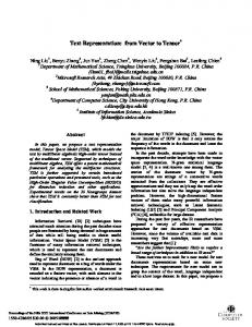
Lifted operators are important for meeting our goal of supporting direct representation of mathematical concepts in Diderot source code. For example, consider trying to visualize the bone surface in a CT scan. The simple, first-order, approach is to render an isosurface. The three images on the left of Figure 1 show Fig. 1. Volume rendering of isocontours (left) how unsatisfactory this is, due to wide and Canny edges (right) from a CT scan of Cevariations in bone density: no isosurface bus apella (capuchin) head. correctly shows the skull. A better way to visualize the bone surface is to use a 3D version of Canny edge detection [6]. Diderot alV lows this math to be used directly in a field definition: field#2(3)[] F = ∇(|∇ V|)·∇ |∇V |; A surface rendering of where F(x) is zero is shown on the right of Figure 2. The entire bone surface is visible, color-mapped by the underlying data value. Particularly significant is the surface shading computed in terms of ∇F , which requires a third derivative of V. Using the product and chain rules of differentiation, the compiler generated all the code needed to reconstruct and manipulate ∇ ⊗ ∇ ⊗ ∇ V, a third-order tensor. V=3000

V=2150

3300

1200

V=1300

5

EIN

To address this limitation of direct-style tensor operations, we have developed a new intermediate representation, that we call EIN, which is much more compact than the full expansion of tensor expressions (such as the matrix in Equation 3), while permitting index-specific operations. This new representation is embedded in the same SSA-based representation as the direct-style operators, except that we now have EIN assignment nodes of the form t = λparamsheiα (args) (4) where – t is a tensor or field variable being assigned – λparamsheiα is an operator defined in the EIN IR, with formal parameters params, α is the shape of tensor t, or range of field t, and body e. – args are the argument variables to the EIN operator In an EIN operator, the bound indices range over the shape of the result; i.e., a scalar result has no indices, a vector result has one bound index, a matrix result has two, and so on. One way to think of EIN expressions is that they are a compact way to represent the loop nest that computes their result (although in our compiler we usually unroll their implementation). For example, the expression trace(u⊗v) is represented in High-IR as P t1 = λU, V hUi Vj iij (u,v) t2 = λT h i Tii i(t1 ) (5) where the ranges on the indices are inferred from the types. In this example, it will automatically reduce the expression to P t2 −→ λ(U, V )h i Ui Vi i(u,v) thus discovering the identity trace(u ⊗ v) = u · v. Returning to the curl example, EIN (Figure 2) gives a compact representation DP of the matrix E (Equation 3). ∂ t = λF E F (F) kl ikl ∂xjk l ij

5.1

EIN Notation

EIN operators provide a mathematically sound and compact representation for tensor and field operations. This section introduces the notation used to represent the tensor and field operations in the Diderot compiler that replaces the old direct-style IR. The grammar of EIN operators is given in Figure 2 (we omit the full set of arithmetic operators for compactness). ::= Tα , Aα , Bα | Fα , Gα | vα (e) | hβ (e) Tensor, Field, Image, and Kernel | δij | Eij , Eijk Kronecker deltas, Levi-Civita tensor √ ∂ |  e, lift(e), sine(e), en , e unary operators ∂α | e1 @e2 , e − e, ee , e ∗ e binary operators Pn2 β other operators | α=n1 e, | Vα ~ H . . . µ = i, j, k variable | n ∈ N constant indices α, β, γ = µ ¯ sequence of indices E = λ¯ xheiα EIN Operator e

Fig. 2. The syntax of EIN operators E and EIN expressions e in High-IR

A key aspect of the EIN IR is the tracking of indices. Indices can either be variables (denoted by i, j, and k), or constants (n ∈ N). We also use α, and β to denote sequences of zero or more indices of either type. A variable index can either be bound in a summation or as one of the indices that determine the shape of the EIN operator’s result. EIN expressions include tensors (Tα ), and fields (Fα ); the latter two forms have multi-index subscripts specify the individual component for higher-order shapes. The Levi-Civita symbol (Eij ,Eijk ) and Kronecker delta (δij ) are used to permute and cancel components based on their indices. Summations have the usual semantics (Σν¯ e). There ∂ are several forms that are special to fields. These include differentiation ( ∂α  e), probing (e1 @e2 ), lifting a tensor to represent a constant field (lift(e)), and defining a field as the convolution of an image and a kernel (Vα ~ H β ). Math functions include cosine, sine, arccosine, and arcsine. Lastly, we have the standard arithmetic operations, such as addition and multiplication. In the remainder of this section, we illustrate the constructs of EIN operator by example. Consider the expression λ¯ xh

P

ν

eii

where 0 ≤ i < n and ν = [c ≤ j ≤ d]

which has two indices i, j. The bound index i ranges from 0 to n − 1 and gives the expression its shape (i.e., a vector in Rn ).4 The summation index j ranges from c to d. Each component in the resulting vector (Equation 5.1) binds index i and evaluates e. Permutation tensor and Kronecker delta The Eα and δi,j expressions are the permutation (or Levi-Civita) tensor and Kronecker delta function.We use these to model index-dependent tensor operations. Fields and Tensors EIN expressions describe Fields Fα and Tensors Tα of arbitrary shapes (similar to traditional index notation). A field and tensor expression is appended 4

By convention, we omit the range on bound indices, but they are present in the IR in our compiler.

with a list of indices that refer to the size of the tensor or field. A scalar field is expressed as F , a vector field is expressed as Fi , Tij is a matrix, and Tijk is a second-order tensor. Probe and Lift The probe operator e1 @e2 applies field e1 to the point e2 and lift(e) lifts a tensor e in a field expression. Convolution The convolution expression Vα1 ~ H α2 is the convolution operation of an image field V , with the range α1 and a piecewise polynomial kernel H. Field reconstruction is discussed in more detail in Section 5.4. ∂  e denotes differentiation on field e. The concise Differentiation The expression ∂α representation of differentiation allows us to express a wide variety of differentiation operations including the gradient (∇), divergence (∇·), curl (∇×), Jacobian (∇⊗). 5.2

Generating EIN Expressions

The Diderot compiler generates High-IR, including the EIN operators, from an explicitly typed simplified AST representation. For many related operations, we can define a generic (i.e., shape polymorphic) EIN operator that gets specialized based on its type. A simple example is the tensor addition operator, which works on tensors of any shape. We define a generic tensor addition operation that is parameterized over a multi-index meta-variable α and using de Bruijn numbering: Λαλ(A, B)hAα + Bα iα

(6)

We specialize the operator to a particular shape by replacing α with a multi-index that ranges over the shape. 5.3

Lifted Tensor Operations

One benefit of the EIN IR is that it makes implementing lifted operators (i.e., tensor operations lifted to work on fields) much easier. Consider the inner product operator • lifted to work on fields. It has the generic definition (left-hand side) P P λ(F, G)h k Fαk Gkβ iαβ −→ λ(F, G)h k Fk Gki ii where α and β are specialized to handle different shapes. The inner product between a vector field F and a matrix field G is realized (right-hand side) by instantiating α to the empty multi-index and β to a single index. The result of this computation is a field expression that can be probed, differentiated and used in a visualization algorithm. This flexibility is simply not feasible in the direct style compiler (see Section 4). 5.4

Field Reconstruction

This section will illustrate field reconstruction with EIN and offer an example. During the transition from High-IR to Mid-IR, higher order constructs get replaced by lowerorder constructs. Probed fields v ~ h(x) are replaced with terms to express computation being done on the image separable kernels. Traditional index notation [15] does not provide the notation needed to show the reconstruction of fields. The EIN expressions ¯ vα (¯ e), val(i), and hψ (e) are introduced for this purpose.

Design The expression vα denotes an image field. The expression vα [¯ e] is an image field indexed at a list of integer positions e ¯ . The val(i) notation lifts an index variable to Pn a constant integer; e.g., i=0 val(i) = 0 + 1 + 2 + · · · + n. We use the notation hn to ¯ refer to the nth derivative of univariate function h. In EIN expression hψ the level and ¯ which is a list of pairs [(c, i1 ), . . . , (c, im )] type of differentiation is captured in the ψ, that are evaluated like Kronecker-deltas pairs (i.e., ψ = (c, i) = δc,i ) and added together. Implementation We build on the exposition in [8], reproduced here for convenience, to explain the context and contribution of EIN. Let f be a 2-d vector field field#0(2)[2] F = tent ~ img("i.nrrd"); vec2 out = F(p); The output of probing vector field is evaluated as  Ps  v0 [n0 + i, n1 + j]h(f0 − i)h(f1 − j) Pij:1−s (7) s ij:1−s v1 [n0 + i, n1 + j]h(f0 − i)h(f1 − j) In High-IR this operation is represented as a single EIN operator out = λ(V, H, T )hVi ~ H(T )ii (F, tent, p) where and 0 ≤ i ≤ 1

(8)

Position p is in world-space and is transformed to image-space position x using transformation matrix M and translation matrix T. R = M−1

x = λ(A, B, C)hΣj (Aij Bj ) + Ci ii (R, p, T)

n = bxc

f=x−n

The transformation between basis were previously represented with direct-style operators that generated function calls. Now they can be represented with mix of simple direct-style and EIN operators. The field (equation 8) is reconstructed in EIN notation as out −→ λ(v, h, n, f )heiα (F, tent, n, f) Ps e = jk=1−s vα [n0 + val(j), n1 + val(k)]h(f0 − val(j))h(f1 − val(k)) The specific axis for the fractional f and integer n position are represented with a constant index. Variable indices are lifted to integer values as val(i) and val(j). Differentiation The differentiation of a field is pushed down to the polynomial kernels. Our general approach allows us to represent, reconstruct, and normalize ∇α rather than it’s many variations. In EIN notation we express (1) as ∇i H(x, y) = hδ0i (x)hδ1i (y)

6

(9)

Optimization and Transformations

This section offers a unique set of techniques organized around the EIN IR that makes compilation possible. The previous section described the design of our IR to represent operations between tensor and tensor fields. The translation from tensor field operators to low-level executable code has brought technical challenges. A naive implementation of our transformations causes unacceptable space blowup. To address this we have developed techniques around the IR to reduce and the size from lowering passes. As discussed in the previous section, surface language operators are mapped to EIN operators. From there we use substitution, a systematic way to apply EIN operators to

one another, followed by the rewriting system that normalizes EIN operators. After the normalization process EIN expressions can be rather large and complicated. This can make it difficult to efficiently generate code, take advantage of vector hardware, and eliminate redundant expressions. To address these concerns we introduce techniques Shift, Split, and Slice, and demonstrate it’s application. As a side effect, the rewriting does let us discover algebraic identities. Figure 3 list some examples of identities. 6.1

Substitution

We describe the act of substitution by example, starting with tensors a and b with shape γ, tensor s with shape α, operations t1 = a + b and t2 = s ⊗ t1 . The terms are expressed in High-IR as two EIN operators t1 = λ(A, B)hAγ + Bγ iγ (a, b)

t2 = λ(S, T )hSα Tβ iαβ (s, t1 )

The High-IR optimization phase will combine these operators into one EIN operator. The result is a single EIN operator to represent these two operations. t2 −→ λ(S, A, B)hSα (Aβ + Bβ )iαβ (s, a, b) where γ is instantiated with β This process allows us to represent computations on fields with a single expressions, which can then be normalized and treated generically by the rewriting system. Rewrites ∇ × ∇ϕ =⇒ 0, ∇ · (∇×F) =⇒ 0 (a ×b )×c =⇒b (a ·c )−a (b ·c ) (a ×b )×(c ×d) =⇒(a ·(c ×d )b) − (b ·(c ×d )a) (a ×b )·(c ×d) =⇒(a ·c) (b ·d) − (a ·d) (b ·c)

Substitution Tr(a⊗b)=⇒ a·b ∇ ⊗ (∇ϕ) =⇒ ∇ ⊗ ∇ϕ Tr(∇ ⊗ ∇ϕ) =⇒ ∇2 ϕ (MT )T =⇒ M

Fig. 3. This table is a list of identities that can be found from term rewriting and the substitution technique. The tensors and fields are written in surface language syntax where ϕ is a scalar field, M is a second-order tensor field, F is a generic fields, and a,b,c,d are vectors

6.2

Normalization

Transformation rules serve to simplify expressions by normalizing field terms, applying differentiation, and optimizing expressions. Field Normalization includes pushing probes down to convolution and differentiation down to kernels. By pushing the field expression past tensor operators and down to the field term, the operators are computed on the tensor result of a probe rather than the entire field. (sFβ )(x) =⇒ s(Fβ (x))

sine(Fα )@x =⇒ sine(Fα @x)

The differentiation index is pushed down to the kernels in a convolution expression. The direct style version of this rule (1) limited the type of differentiation that can be supported, so instead EIN notation has the following rewrite ∂  (Vα ~ H β ) =⇒ Vα ~ H βµ (10) ∂xµ

Differentiation is a necessary step to translate generic EIN expressions to into realizable field terms. The rewrites follow the rules of tensor calculus. They include the product rule, quotient rule, chain rule, power rule, and certain trigonometric identities. e1 (∇  e1 )e2 − e1 (∇  e2 ) ∇  (e1 e) =⇒ e1 (∇  e) + e(∇  e1 ) ∇ =⇒ e2 e22 Index based optimizations are possible with EIN notation. Applying one of these optimizations reduces on at least one index and effectively removes at least one summation loop from the operation. The differentiation indices could have two of the same variable index as an epsilon ∇ij  (Eijk e) =⇒ 0.0 This rewrite enables the compiler to find identities ∇ × ∇ϕ =⇒ 0 and ∇ · ∇ × F =⇒ 0. Two epsilons in an expression with a shared index can be rewritten to deltas [10]. Eijk Eilm =⇒ δjl δkm − δjm δkl

(11)

A δij expression can be applied to tensors, fields, and the del operator. δij Tj =⇒ Ti 6.3

δij Fj =⇒ Fi

∇j  δij e =⇒ ∇i  e

(12)

Shift

The Shift method leverages EIN notation to effectively move terms embedded in a summation operation, much like moving invariant terms outside of a loop nest. The method works by analyzing the index-dependencies in a generic EIN expression e and the outer summation. Given Σk aj , expression aj is invariant to expression Σk because variable index j 6∈ {k} and so the term is moved outside the summation expression. Consider the following expression P P P e −→ jk (aj bk cj dk ) −→ j (aj cj ) ∗ k (bk dk ) (13) Shift moves the invariant term, a loop, outside the inner loop. The next phase of compiler splits this operator into smaller EIN operators. This makes it easier to find common computations in the rest of the program and take advantage of vector hardware. 6.4

Split

The substitution process can create large complicated expressions that can be difficult to compile. Diderot does value numbering on a global scale but it is insufficient to compiling many of the more mature and complicated Diderot programs. EIN adds a level of complexity to this process because common terms could be bound to different ∇ e variable index or embedded inside a complicated expressions i.e. eij e1k − ∇jk Pk ij . l ell ei2 We have created a Splitting technique to Split any complicated EIN operators into a series of simple small operators. As we split we use Hash consing to share values and effectively find common subexpressions. The Split operation lifts out subexpressions while maintaining information about the indices involved. Given a operation,

t0 = λT he1 ∗ esiα (args), if e1 is another operation(+ − ∗...) then it lifted into a new operator t_1, and the term e1 is replaced with Tβ in t0 . We use HashCons to find if t_1 has been used before . If so, we found a common subexpression and if not we bind the new EIN operator. t1 = λT he1 iβ (args)

t0 = λT hTβ ∗ esiα (t1 , args)

In order to enable splitting we need to be able to impose a concept of shape β of any EIN expression e1 . Unlike tradition index notation, two repeat indices do not imply summation. The shape extracted needs to reflect simple operations A+B. e1 = Aijk + Bijk and β = i, j, k the order that the indices appear Transpose(A⊗B), e1 = Aj Bi and β = j, i if the indices repeat in multiple terms modulate(A,B), e1 = Aij Bij and β = i, j and with P summation operators A ⊗(F· C), e1 = Ai ( k Fk Ckj ) and β = i, j.

6.5

Slice

In the next stage of the compiler, each field expression creates a vast number of lowerlevel operators to index discrete data and evaluate polynomial kernels. Split finds identical field expressions, while Slice identifies field expressions that are not the same but will create many of the same lower level operators. Some operations evaluates components for field terms individually Fx , Fy , Fz . Each component is unique Fx 6= Fy , but may be defined by the same source data and reconstruction can create many of the same computations. Transforming these operations directly can create an IR that is too large to compile. Consider the determinant of a second-order tensor field M tensor[3,3] A = M(p); tensor[] G = det(M)(p); transformed to EIN as A = λ(F, T )hFij (T )iij (M,p) DP E G = λ(F, T ) E F (T )F (T )F (T ) (M,p) ijk 0i 1j 2k ijk

(14)

ij

A naive implementation applied field reconstruction (Section 5.4) on each field term (Fij , F0i , F1i , F2i ) and creates many of the same operations. EIN notation could be used to identify these common computations and change the probe of a sliced field to a tensor operator indexing the original field. For simplicity, we omit the steps for splitting and express the result with some rewriting. DP E A = λ(F, T )hFij (T )iij (M,p) G −→ λ(T ) E T T T (A) (15) ijk 0i 1j 2k ijk ij

Field reconstruction is then only applied to one field term Fij instead of four. The difference can be more significant when considering more complication tensor computations ( ∇ ⊗ ∇det(M)). This technique allows the compiler to transform a smaller representation into low-IR and prevent the blow-up the naive implementation of EIN caused.

7

Benchmarks

We want the Diderot programmer to be able to define a field with a series of lifted operators on the surface language, and rely on the compiler to differentiate it a few times. This level of expressiveness makes writing Diderot code easier, faster, and more intuitive. An earlier paper [18] demonstrated the impact of this work by illustrating visualization features otherwise not available. It is useful to evaluate the impact of this approach on the compiler and the language. In this section, we present three sets of benchmark results. The first set is an evaluation of implementing EIN over the original direct-style compiler. The second set of numbers measures the effect of the techniques described in Section 6. The third is an evaluation of the effect of using the higher-order features of the language versus equivalent first-order implementations. 7.1

Experimental Framework

The benchmarks were run on an Apple iMac with a 2.7 GHz Intel core i5 processor, 8GB memory, and OS X Yosemite (10.10.5) operating system. Each benchmark was run 10 times and we report the average time in seconds. The benchmarks are presented in the figures in order of mathematical complexity. Benchmarks “illust-vr”,“lic2d”,“mandelbrot”,“ridge3d”, and “vr-lite-cam” are small examples available in the original compiler [8]. The benchmarks ,“mode”, “canny”, and ,“moe” are used to create figures in [18], and are discussed in Section 4.2. “Mode” finds lines of degeneracy in a stress tensor field revealed by volume rendering isosurface of tensor mode; “Canny-edges” computes Canny Edges; and “Moe” volume renders isocontours found using Canny Edges (see Section 4.3). Programs with “-first” indicate that derivations were done on paper so the program could be written with first-order operators and could be executed on the original compiler. The benchmarks “dec-crest”, “dec-grad”, “rsvr”, and“mode-rig’ were not featured in previous work, because they were outside the scope of possibility and involved a higher degree of tensor math. Programs “dec-crest” and “dec-grad” are approximations to illustrate the crest lines on a dodecahedron. Programs “mode-rig” and “rsvr” are both programs created to measure ridge lines. The micro-benchmarks “det-grad”,“det-hess”, and “det-trig” compute a single property: The gradient, hessian, and various functions computed on the determinant of a field. Their run times are negligible and are omitted. 7.2

The Effect of implementing EIN

Figure 4 compares the application of EIN with the original compiler. Many of the benchmarks could not be expressed in the previous version of the language and are indicated in the graph. The development of EIN has impacted the type and complexity of programs that be implemented with Diderot. Figure 4 illustrates the measurements for all the benchmarks with full or a restricted level of the optimizations mentioned in this paper. The next section will take a closer look at the impact of individual techniques. Here we can summarize that fully implementing the optimizations enables Diderot to compile programs that otherwise can not compile, and can compile programs faster, while also offering faster or comparable executables.

Time%(log%s)

100 10 1

Original

Ein.with.restrictions

EIN

Ein.with.restrictions

rsvr

modeCrig

decChess

EIN

100

Time%(log%s)

100 10

10

Programs

moeChigh

EIN cannyChigh

modeCfirst

moeCfirst

No(slice(

illustCvr

ridge3d

Minimal(Split

cannyCfirst

100

Slice%and%Split:%Compile%Times vrCliteCcam

Time%(log%s)

rsvr

modeCrig

decChess

detCtrig

decCgrad

detChess

detCgrad

moeChigh

modeChigh

cannyChigh

moeCfirst

modeCfirst

illustCvr

cannyCfirst

ridge3d

vrCliteCcam

lic2d

mandelbrot

Programs

mandelbrot

1 1000

modeChigh

1 0.1

lic2d

Time%(log%s)

1000

Original

detCtrig

Programs

Design%of%EIN:%Run%Times

Design%of%EIN:%Compile%Times

decCgrad

detChess

detCgrad

moeChigh

modeChigh

cannyChigh

moeCfirst

modeCfirst

illustCvr

cannyCfirst

ridge3d

vrCliteCcam

lic2d

mandelbrot

0.1

rsvr

mode5rig

dec5hess

det5trig

dec5grad

det5hess

det5grad

moe5high

Slice%and%Split:%Run%Times

Minimal(split

No(slice(

EIN

100

Time%(log%s)

modeChigh

Programs

moeChigh

modeCfirst

EIN cannyChigh

cannyCfirst

moeCfirst

No(slice(

illustCvr

ridge3d

lic2d

100

vrCliteCcam

Minimal(Split

1

mandelbrot

10

10

1

dec5grad

mode5high

Programs

moe5high

canny5high

rsvr

mode5rig

dec5hess

det5trig

dec5grad

det5hess

det5grad

moe5high

mode5high

canny5high

mode5first

moe5first

canny5first

Programs

mode5first

0.1

1

canny5first

Time%(log%s)

mode5high

The Effect of Compiler Settings Slice%and%Split:%Compile%Times

1000

Programs

10

moe5first

Time%(log%s)

7.3

mode5first

EIN

canny5high

Ein.with.restrictions

100

moe5first

Original

canny5first

10 Fig. 4. The “Original”version of the compiler does not use the EIN IR. “Restricted” is the more naive implementation of EIN. “EIN” is the baseline with the EIN IR with full optimizations 1 applied. Design%of%EIN:%Run%Times

Time%(log%s)

Fig. 5. Compile and run time measurements when implementing Slice and Split on High-IR. Slice%and%Split:%Run%Times Doing no amount of splitting prevents most of these programs from compiling so instead we Minimal(split No(slice( EIN 100 measure its impact by limiting it, “Minimal Split”. EIN is the baseline with techniques Split and Slice implemented. 10 1

As we have discussed previously, a na¨ıve application of our transformations causes unacceptable space blowup. To address this problem we developed techniques to reduce the size of the IR resulting from lowering passes. While their implementation might allow more complicated Diderot programs to be created we want to evaluate the cost or Programs benefit it might impose on the programs that could already compile. In this section, we evaluate the effectiveness of these techniques together and isolated at different levels of abstraction. Figures 5 and 6 measures the effectiveness of applying Split (Section 6.4) and Slice (Section 6.5) on a high-IR EIN operator. Both techniques are effective at reducing the size of the program by finding common subexpressions or reducing field terms (Figure 6). The slice technique is necessary to compile 3 of the 14 benchmarks. Split is the most consequential technique (Figure 5). Restricting it stops 5 of the programs from being able to compile. Neither technique assert a considerable cost to execution time. We measured the effect of optimizations on a specific operation transformation at a lower level of abstraction. Figure 7 measures the application of the optimizations on reconstructed field terms.Applying optimizations Shift and Split together offers a consistent speed-up on the execution time and compile time for all 13 benchmarks. 5 dec5grad

mode5high

moe5high

canny5high

mode5first

moe5first

canny5first

0.1

Size$of$rsvr$program Restricted

Minimal.Split

No.Shift

No.Slice

EIN

log$(Size/1000)

10000

1000

100

10

1

1

2

3

Phase

4

5

6

Size$of$dec9grad$program Restricted

Minimal.Split

Size$of$rsvr$program

No.Shift

EIN/No.Slice

10000

Time%(log%s)

1000

100

log$(Size/1000)

EIN

1000

100

100

10

10

3

4

Phase

5

rsvr

2

mode5rig

1

dec5hess

1

det5trig

6

dec5grad

5

det5hess

4

det5grad

Phase

moe5high

3

mode5high

2

canny5high

1

canny5first

1

moe5first

10

1

mode5first

log$(Size/1000)

1000

Restricted Minimal.Split No.Shift No.Slice Shift%and%Split:%Compile%Times 10000 No)Split)and)No)Shift No)Shift EIN

6

Programs

Fig. 6. The graphs shows the size of the dec-grad (left) and rsvr program (right) program at Size$of$dec9grad$program Restricted No.Shift EIN/No.Slice different phases in the compiler. “EIN” is the baseline with fullMinimal.Split optimizations. No)Split)and)No)Shift

1000

No)Shift

log$(Size/1000) Time%(log%s)

10000

Shift%and%Split:%Compile%Times

EIN

Shift%and%Split:%Run%Times

No)Split)and)No)Shift

1000

No)Shift

EIN

100

Time%(log%s)

100

100

10

10 10

1 1

5

First,order.on.Ein Programs

High,order.on.Ein

Time%(log%s)

100

dec5grad

First%vs.%High%order:%Compile%Times

First,order.on.Original

Programs

6

mode5high

4

moe5high

Phase

canny5high

3

mode5first

2

canny5first

rsvr

mode5rig

dec5hess

det5trig

dec5grad

det5hess

det5grad

moe5high

mode5high

canny5high

moe5first

mode5first

canny5first

1

moe5first

0.1

1

Fig. 7. Shift and Split on Mid-IR. Compile and run time measurements for implementing Shift 10 and Split techniques on reconstructed field terms. EIN baseline includes the application of Shift Shift%and%Split:%Run%Times and Split. No)Split)and)No)Shift No)Shift EIN mode

10

moe

1

canny

Time%(log%s)

100

programs experienced at least a 20x compile time speed-up. 4Programs of the 7 benchmarks offered at least a 1.3 speed up on execution time while the rest were comparable. 1

First%vs.%High%order%program:%RunTimes

rsvr

mode5rig

dec5hess

dec5grad

First,order.on.Ein

First,order.on.Original

High,order.on.Ein

First,order.on.Ein

High,order.on.Ein

100

Programs

Time%(log%s)

10

10

Programs

mode

mode

moe

canny

Programs

moe

1

1

canny

Time%(log%s)

100

mode5high

First,order.on.Original

moe5high

mode5first

canny5high

First%vs.%High%order:%Compile%Times

moe5first

canny5first

0.1

Fig. 8. This figure compares hand-derived first-order programs with their high-order equivalent, and first-order programs on the original compiler and with EIN. First%vs.%High%order%program:%RunTimes First,order.on.Original

First,order.on.Ein

High,order.on.Ein

Time%(log%s)

100

7.4

10

First-Order versus Higer-Order

High-order versions of program are the preferred way to write Diderot code. Their firstorder counterparts require Programs more lines of code and makes the user do derivations by hand. The process can be time-consuming, tedious, and error-prone. Figure 8 reports the compile and run time for first-order programs with their higher order counterparts. mode

moe

canny

1

The measurements are comparable for first and higher order programs ran with EIN. Lastly, first-order implementations of the program compiled and ran faster on EIN than on the original compiler.

8

Conclusion

We introduced and described the design of our IR, and some of the technical challenges in efficiently managing the translation from tensor fields to low-level executable code. The work enables a richer set of algorithms that can be created with Diderot. This makes programming in Diderot easier, faster, and more intuitive. We intend to continue developing the work to push the boundaries for what Diderot can do, while assuring the user of the correctness of the work.

References 1. K. Ahlander. Einstein summation for multi-dimensional arrays. Computers and Mathematics with Applications, 44:1007–1017, October – November 2002. 2. Martin S. Alnaes, Anders Logg, Kristian B. Oelgaard, Marie E. Rognes, and Garth N. Wells. Unified form language: A domain-specific language for weak formulations of partial differential equations. ACM Transactions on Mathematical Software(TOMS), 40, 2014. 3. A. Barr. The Einstein summation notation, introduction to cartesian tensors and extensions to the notation. Draft paper; available at http://zeus.phys.uconn.edu/ mcintyre/workfiles/Papers/Einstien-Summation-Notation.pdf. 4. P J Basser and C Pierpaoli. Microstructural and physiological features of tissues elucidated by quantitative-diffusion-tensor MRI. Journal of Magnetic Resonance, Series B, 111(3):209– 219, 1996. 5. Kevin J. Brown, Arvind K. Sujeeth, HyoukJoong Lee, Tiark Rompf, Hassan Chafi, Martin Odersky, and Kunle Olukotun. A heterogeneous parallel framework for domain-specific languages. In Proceedings of the 20th International Conference on Parallel Architectures and Compilation Techniques (PACT ’11), October 2011. 6. J. Canny. A computational approach to edge detection. IEEE Trans Pattern Analysis and Machine Intelligence, 8(6):679–714, 1986. 7. Hassan Chafi, Zach Devito, Adriaan Moors, Tiark Rompf, Arvind K. Sujeeth, Pat Hanrahan, Martin Odersky, and Kunle Olukotun. Language virtualization for heterogeneous parallel computing. In Proceedings of the 2010 ACM SIGPLAN Conference on Object-oriented Programming Systems, Languages, and Applications (OOPSLA ’10), pages 835–847, October 2010. Part of the Onward! 2010 Conference. 8. Charisee Chiw, Gordon Kindlmann, John Reppy, Lamont Samuels, and Nick Seltzer. Diderot: A parallel DSL for image analysis and visualization. In Proceedings of the 2012 SIGPLAN Conference on Programming Language Design and Implementation (PLDI ’12), pages 111–120, New York, NY, June 2012. ACM. 9. Hyungsuk Choi, Woohyuk Choi, Tran Minh Quan, David G. C. Hildebrand, Hanspeter Pfister, and Won-Ki Jeong. Vivaldi: A domain-specific language for volume processing and visualization on distributed heterogeneous systems. IEEE Transactions on Visualization and Computer Graphics (Proc. SciVis), 20(12):2407–2416, December 2014. 10. Tai L. Chow. Mathematical Methods for Physicists : A Concise Introduction. Cambridge University Press, Cambridge, 2000.

11. D. Cociorva, J. Wilkins, C. Lam, G. Baumgartner, P. Sadayappan, and J. Ramanujam. Loop optimizations for a class of memory-constrained computations. Proceedings of the 15th ACM International Conference on Supercomputing, pages 103–113, 2001. 12. Ron Cytron, Jeanne Ferrante, Barry K. Rosen, Mark N. Wegman, and F. Kenneth Zadeck. Efficiently computing static single assignment form and the control dependence graph. ACM Transactions on Programming Languages and Systems, 13(4):451–490, Oct 1991. 13. D. Degani, Y. Levy, and A. Seginer. Graphical visualization of vortical flows by means of helicity. American Institute of Aeronautics and Astronautics (AIAA) Journal, 28:1347–1352, August 1990. 14. Kees Dullemond and Kasper Peeters. Introduction to Tensor Calculus. Kees Dullemond and Kasper Peeters, 1991. 15. Albert Einstein. The foundation of the general theory of relativity. In A. J. Kox, Martin J. Klein, and Robert Schulmann, editors, The Collected papers of Albert Einstein, volume 6, pages 146–200. Princeton University Press, Princeton NJ, 1996. 16. Charles Hansen and Christopher R. Johnson, editors. The Visualization Handbook. Academic Press, 2004. 17. Miloˇs Haˇsan, John Wolfgang, George Chen, and Hanspeter Pfister. Shadie: A domain-specific language for volume visualization. Draft paper; available at urlhttp://miloshasan.net/Shadie/shadie.pdf, 2010. 18. Gordon Kindlmann, Charisee Chiw, Nicholas Seltzer, Lamont Samuels, and John Reppy. Diderot: a domain-specific language for portable parallel scientific visualization and image analysis. IEEE Transactions on Visualization and Computer Graphics (Proceedings VIS 2015), 22(1):867–876, January 2016. 19. F. Luporini, A.L. Varbanescu, F. Rathgeber, G.-T. Bercea, J. Ramanujam, D.A. Ham, and P.H.J. Kelly. Cross-loop optimization of arithmetic intensity for finite element local assembly. ACM Transactions on Architecture and Code Optimization (TACO), 11(4):Article No. 57, January 2015. 20. Patrick McCormick, Jeff Inman, James Ahrens, Jamaludin Mohd-Yusof, Greg Roth, and Sharen Cummins. Scout: A data-parallel programming language for graphics processors. J. Par. Comp., 33:648–662, November 2007. 21. M. Puschel, J.M.F. Moura, J.R. Johnson, D. Padua, M.M. Veloso, B.W. Singer, J. Xiong, F. Franchetti, A. Gacic, Y. Voronenko, K. Chen, R.W. Johnson, and N. Rizzolo. SPIRAL: Code generation for DSP transforms. Proceedings of the IEEE, 93(2):232–275, February 2005. 22. Peter Rautek, Stefan Bruckner, M. Eduard Gr¨oller, and Markus Hadwiger. ViSlang: A system for interpreted domain-specific languages for scientific visualization. IEEE Transactions on Visualization and Computer Graphics (Proc. SciVis), 20(12):2388–2396, December 2014. 23. James. Simmonds. A Brief on Tensor Analysis. Springer-Verlag, New York, 1982. 24. Ivan Stephen Sokolinkoff. Tensor Analysis. John Wiley and Sons, New York, 1960. 25. Teem Library. Teem website at http://teem.sf.net.