Elastic properties of a two-dimensional model of crystals containing ...

PHYSICAL REVIEW B, VOLUME 65, 094101

Elastic properties of a two-dimensional model of crystals containing particles with rotational degrees of freedom Aleksey A. Vasiliev,1 Sergey V. Dmitriev,2,* Yoshihiro Ishibashi,3 and Takeshi Shigenari2 1

Department of Mathematical Modeling, Tver State University, 33 Zhelyabov Street, 170000 Tver, Russia 2 Department of Applied Physics and Chemistry, University of Electro-Communications, Chofu-shi, Tokyo 182-8585, Japan 3 Faculty of Communications, Aichi Shukutoku University, Nagakute-Katahira 9, Nagakute-cho, Aichi Prefecture 480-1197, Japan 共Received 4 July 2001; published 28 January 2002兲 We consider a discrete two-dimensional model of a crystal with particles having rotational degrees of freedom. We derive the equations of motion and analyze its continuum analog obtained in the long-wave limit. The continuum equations are shown to be the ones of the micropolar elasticity theory. The conditions when the micropolar elasticity equations can be reduced to the equations of conventional elasticity theory are discussed. We show that the rotational degrees of freedom are responsible for the anomalies in the elastic properties of some of the dielectric crystals. DOI: 10.1103/PhysRevB.65.094101

PACS number共s兲: 77.84.⫺s, 62.20.Dc, 46.05.⫹b

I. INTRODUCTION

In many dielectric crystals the atom clusters are put together to form a lattice and the forces that hold the clusters together are usually much weaker compared to intercluster forces. It is natural to assume for such crystals that atom clusters are rigid: that is, to neglect the high-frequency intercluster vibrations. The positions of a finite-size cluster is defined not only by the displacement vector but also by the orientation angles. Coupling of the translational and rotational degrees of freedom may result in the appearance of soft optic modes. Contributions of the rotational modes to the physics of dielectric crystals have been studied from a continuum viewpoint1– 4 and with the use of microscopic models.2,5–9 The role of rigid unit modes 共RUM’s兲 in amorphous and crystalline silica has been studied in Ref. 10. The theory of the coupling of an electric field with a field of elastic strain has been developed by Sannikov.11 In the present paper we focus on unusual elastic properties exhibited by the crystals with particles having rotational degrees of freedom. Particularly, we examine the nature of the negative Poisson ratio ( ␯ ) in such crystals. The Poisson ratio characterizes the response of an elastic body to uniaxial stress and is defined as the negative ratio between the transverse strain and the corresponding axial strain. For most of the materials in nature ␯ lies in the range from 0 to 0.5 and normally it is nearly equal to 0.3. Practically zero ␯ is exhibited, for example, by cork, and ␯ ⫽0.5 共constant volume medium兲 is observed for rubber or for the plastic deformation of metals. An elastic medium can be stable only if the Lame coefficients are positive.12 This suggests that the Poisson ratio of an isotropic elastic medium can range from ⫺1 to 0.5. For an anisotropic medium, ␯ can take any value in some particular directions. That is why the negative ␯ is often attributed to the anisotropy of medium.13 The anisotropy is the reason for the negative ␯ in highly anisotropic crystals like arsenic, antimony, and bismuth14 and also in many single crystals of cubic metals deformed in an oblique direction 0163-1829/2002/65共9兲/094101共7兲/$20.00

with respect to the cubic axis.15 However, isotropic materials with negative ␯ are quite rare. Cubic metals in the polycrystalline 共isotropic兲 state show ␯ of about 0.3. It seems that the negative ␯ in an isotropic medium can be explained through the rotational degrees of freedom. The examples are the foams16,17 and quartz 共isotropic in the XY plane兲 near the ␣ -␤ phase transition.18 In auxetics the negative Poisson ratio can be explained by their special electronic structure.19 An anomaly in the Poisson ratio has been reported for an isotropic two-dimensional 共2D兲 microscopic model by Wojciechowski.8 In his model ␯ becomes negative at high densities. A negative Poisson ratio has been reported for a model with rigid and elastic links randomly placed on a 2D honeycomb network near the percolation threshold.20 The possibility to obtain an arbitrary ␯ in an anisotropic 2D microscopic model has been proved in Ref. 21. The model studied in Ref. 21 is a 2D generalization of the elastically hinged molecule 共EHM兲 model.22–24 Another anisotropic 2D model with particles having rotational degrees of freedom has been offered by Ishibashi and Iwata25 in order to describe some properties of the KH2 PO4 共KDP兲 family of crystals, which has been studied extensively in the last five decades.26 Their model contains the rigid particles square in shape, which stand for PO4 tetrahedra. The model explains the variation of ␯ from ⫺1 to 0. Here we carry out a more elaborate study of this model. We analyze the elastic properties of the anisotropic model subjected to homogeneous strain; then we analyze the dispersion relations of the discrete model in comparison with the dispersion relations of two different continuum approximations. The paper is organized as follows. In Sec. II we describe the model and in Sec. III the Hamiltonian and the equations of motion are given. Section IV is devoted to an analysis of the homogeneous strain. In Sec. V the dispersion relations of the microscopic model are derived, and in Sec. VI the discrete model is reduced to the continuum one and, under certain assumptions, to the anisotropic elasticity theory. In Sec. VII the dispersion relations for continuum models are de-

65 094101-1

©2002 The American Physical Society

VASILIEV, DMITRIEV, ISHIBASHI, AND SHIGENARI

PHYSICAL REVIEW B 65 094101

one particle 关square area defined by the centers of particles (m⫺1,n⫺1), (m,n⫺1), (m,n), and (m⫺1,n)兴. III. HAMILTONIAN AND EQUATIONS OF MOTION

We introduce the new variables

␾ m,n ⫽ 共 ⫺1 兲 m⫹n ␸ m,n .

共2兲

Then, the energy of the model can be written as H⫽

1 2

兺 m,n

再

2 2 2 2 ˙ m,n M u˙ m,n ⫹M v˙ m,n ⫹J ␾ ⫹C ␾ m,n

⫹C 1 关 u m,n ⫺u m⫺1,n ⫺A 共 ␾ m,n ⫹ ␾ m⫺1,n 兲兴 2 ⫹C 1 关v m,n ⫺ v m,n⫺1 ⫺A 共 ␾ m,n ⫹ ␾ m,n⫺1 兲兴 2

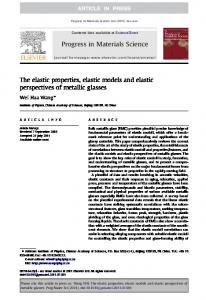
FIG. 1. The 2D microscopic model of a crystal. Absolutely rigid square particles are bound elastically and each particle experiences the action of the rotational background potential. The lattice spacing is h, and a and ␣ are the size and the orientation angle of particles, respectively.

rived and, in Sec. VIII, they are compared to that of the discrete model.

2

⫹

C2 共 u m,n ⫺ v m,n ⫺u m⫺1,n⫹1 ⫹ v m⫺1,n⫹1 兲 2 , 2

冎

⫺ ␾ m⫺1,n 兲 ⫹

C2 共 u m⫹1,n⫹1 ⫹u m⫺1,n⫺1 ⫹u m⫹1,n⫺1 2

⫹u m⫺1,n⫹1 ⫺4u m,n 兲 ⫹

C2 共 v m⫹1,n⫹1 ⫹ v m⫺1,n⫺1 2

⫺ v m⫹1,n⫺1 ⫺ v m⫺1,n⫹1 兲 , a sin ␣ ,

共3兲

where the first three terms give the kinetic energy, the fourth term gives the energy of the rotational on-site potential, the following two terms give the energy of the vertex-to-vertex bonds, and the last two terms give the energy of center-tocenter bonds. Then, the equations of motion are

We consider the 2D microscopic model of a crystal shown in Fig. 1. The model consists of absolutely rigid elastically bound square particles and each particle experiences the action of the rotational background potential. The geometry of the model can be described by the two parameters: the lattice spacing h and the parameter A⫽

C2 共 u m,n ⫹ v m,n ⫺u m⫺1,n⫺1 ⫺ v m⫺1,n⫺1 兲 2 2

M u¨ m,n ⫽C 1 共 u m⫹1,n ⫺2u m,n ⫹u m⫺1,n 兲 ⫺C 1 A 共 ␾ m⫹1,n

II. DESCRIPTION OF THE MODEL

冑2

⫹

共1兲

where a and ␣ are the size and the orientation angle of particles, respectively. Particles have mass M and moment of inertia J. Each particle experiences the action of the rotational background potential with coefficient C. Elastic bonds with coefficient C 1 connect the vertices of each particle with the vertices of nearest neighbors. Elastic bonds with coefficient C 2 connect the center of each particle with the centers of next-nearest neighbors. We are interested here in the elastic properties of the model so that we do not introduce any anharmonic terms. Particles are numbered with two indices m and n. Each particle has three degrees of freedom, namely, two components of displacement vector from the lattice point, u m,n , v m,n , and the angle of rotation, ␸ m,n . A translational cell of the model 关square area defined by the centers of particles (m,n⫺1), (m⫹1,n), (m,n⫹1), and (m⫺1,n)兴 contains two particles. However, the primitive cell contains only

共4兲

M v¨ m,n ⫽C 1 共 v m,n⫹1 ⫺2 v m,n ⫹ v m,n⫺1 兲 ⫺C 1 A 共 ␾ m,n⫹1 ⫺ ␾ m,n⫺1 兲 ⫹

C2 共 u m⫹1,n⫹1 ⫹u m⫺1,n⫺1 ⫺u m⫹1,n⫺1 2

⫺u m⫺1,n⫹1 兲 ⫹

C2 共 v m⫹1,n⫹1 ⫹ v m⫺1,n⫺1 2

⫹ v m⫹1,n⫺1 ⫹ v m⫺1,n⫹1 ⫺4 v m,n 兲 ,

共5兲

¨ m,n ⫽⫺C 1 A 2 共 ␾ m⫹1,n ⫹ ␾ m⫺1,n ⫹ ␾ m,n⫹1 ⫹ ␾ m,n⫺1 J␾ ⫹4 ␾ m,n 兲 ⫹C 1 A 共 u m⫹1,n ⫺u m⫺1,n ⫹ v m,n⫹1 ⫺ v m,n⫺1 兲 ⫺C ␾ m,n .

共6兲

The two first equations give the balance of force components and the third one gives the balance of moments acting on (m,n)th particle.

094101-2

ELASTIC PROPERTIES OF A TWO-DIMENSIONAL . . .

PHYSICAL REVIEW B 65 094101

IV. HOMOGENEOUS STRAIN

Let us subject the model to the homogeneous strain with the components ␧ xx ,␧ y y ,␧ xy , and ␧ yx . The displacements of particles in this case can be written as u m,n ⫽hm␧ xx ⫹hn␧ xy ,

v m,n ⫽hn␧ y y ⫹hm␧ yx ,

␾ m,n ⫽ ␾ .

共7兲

The unknown angle of rotation ␾ can be found from Eq. 共6兲 rewritten in view of Eq. 共7兲 in the form ⫺8C 1 A 2 ␾ ⫹2C 1 Ah 共 ␧ xx ⫹␧ y y 兲 ⫺C ␾ ⫽0.

共8兲

The solution reads

␾⫽

2C 1 Ah 共 ␧ xx ⫹␧ y y 兲 C⫹8C 1 A 2

共9兲

.

Equations 共7兲 and 共9兲 define the displacements of particles in the model under homogeneous strain with components ␧ xx , ␧ y y , ␧ xy , and ␧ yx . To analyze the anisotropy of the model let us calculate the components of the stress tensor in the coordinate system X ⬘ Y ⬘ rotated with respect to the system XY by angle ␤ 共see Fig. 1兲. The result reads

␴ x ⬘ x ⬘ ⫽c 11␧ x ⬘ x ⬘ ⫹c 12␧ y ⬘ y ⬘ ⫹c 13␧ x ⬘ y ⬘ , ␴ y ⬘ y ⬘ ⫽c 21␧ x ⬘ x ⬘ ⫹c 22␧ y ⬘ y ⬘ ⫹c 23␧ x ⬘ y ⬘ , ␴ x ⬘ y ⬘ ⫽ ␴ y ⬘ x ⬘ ⫽c 31␧ x ⬘ x ⬘ ⫹c 32␧ y ⬘ y ⬘ ⫹c 33␧ x ⬘ y ⬘ ,

共10兲

where c i j ⫽c ji with c 11⫽c 22⫽E 1 共 cos4 ␤ ⫹sin4 ␤ 兲 ⫹2 共 E 2 ⫹2E 3 兲 cos2 ␤ sin2 ␤ , c 12⫽2 共 E 1 ⫺2E 3 兲 cos2 ␤ sin2 ␤ ⫹E 2 共 cos4 ␤ ⫹sin4 ␤ 兲 , c 13⫽⫺c 23⫽ 共 ⫺E 1 ⫹E 2 ⫹2E 3 兲 sin ␤ cos ␤ 共 cos2 ␤ ⫺sin2 ␤ 兲 , c 33⫽2 共 E 1 ⫺E 2 兲 cos2 ␤ sin2 ␤ ⫹E 3 共 cos2 ␤ ⫺sin2 ␤ 兲 2 ,

共11兲

and the macroscopic elastic constants are related to the microscopic parameters as follows: E 1 ⫽C 2 ⫹

CC 1 ⫹4C 21 A 2 C⫹8C 1 A 2

,

E 2 ⫽C 2 ⫺

E 3 ⫽C 2 .

FIG. 2. Poisson ratio ␯ ⬘ as the function of orientation angle ␤ of the applied uniaxial stress for A⫽0.5 and different sets of C,C 1 ,C 2 . Curve 1 corresponds to C⫽1, C 1 ⫽1, C 2 ⫽1. Curve 2 is for C⫽100, C 1 ⫽1, C 2 ⫽1. Relatively large C means that particles almost do not rotate. Curves 3 and 4 are for C⫽1, C 1 ⫽100, C 2 ⫽1 and C⫽1, C 1 ⫽1, C 2 ⫽100, respectively.

4C 21 A 2 C⫹8C 1 A

␯ ⬘ ⫽⫺

2 c 12c 33⫹c 13 2 c 11c 33⫺c 13

共13兲

.

Analysis of Eq. 共13兲 shows that ␯ ⬘ is negative if and only CC 21 tg2 共 2 ␤ 兲 ⫹4CC 22 ⫹16C 1 C 2 共 2C 2 ⫺C 1 兲 A 2 ⬍0. 共14兲 One can see that this condition cannot be satisfied in the absence of the rotational degrees of freedom (A⫽0 or C →⬁). Note that many crystals of KDP family demonstrate the negative Poisson ratio.27 It is possible to demonstrate that ⫺1⬍ ␯ ⬘ ⬍1 for any positive C, C 1 , and C 2 and for any A and ␤ . In Fig. 2 we plot ␯ ⬘ as the functions of ␤ for A⫽0.5 and different sets of C, C 1 , and C 2 . Curve 1 corresponds to C⫽1, C 1 ⫽1, and C 2 ⫽1. Curve 2 is for C⫽100, C 1 ⫽1, and C 2 ⫽1. Relatively large C means that particles almost do not rotate. Curve 3 is for C⫽1, C 1 ⫽100, and C 2 ⫽1. In this case, the Poisson ratio is negative in a wide range of uniaxial stress orientations. Curve 4 is for C⫽1, C 1 ⫽1, and C 2 ⫽100. Uniaxial stress along two high-symmetry directions ␤ ⫽0 and ␤ ⫽ ␲ /4 does not cause the appearance of shear strain. For, example, the Poisson ratio for uniaxial stress along ␤ ⫽0 is

, 2

In the coordinate system XY ( ␤ ⫽0), one has E 1 ⫽c 11 , E 2 ⫽c 12 , and E 3 ⫽c 33 . Let us calculate the Poisson ratio, which characterizes the response of elastic body to uniaxial stress and is defined as the negative ratio between the transverse strain and the corresponding longitudinal strain. We put ␴ x ⬘ x ⬘ ⫽0 and ␴ y ⬘ y ⬘ ⫽ ␴ x ⬘ y ⬘ ⫽ ␴ y ⬘ x ⬘ ⫽0, and find from Eq. 共10兲

␧ x⬘x⬘

⫽

if

␯ ␤ ⫽0 ⫽

共12兲

␧ y⬘y⬘

¯ 2 ⫺4C ¯ 21 A 2 ⫹8C ¯ 1C ¯ 2A 2 C ¯ 1 ⫹C ¯ 2 ⫹4C ¯ 21 A 2 ⫹8C ¯ 1C ¯ 2A 2 C

,

共15兲

¯ 1 ⫽C 1 /C and C ¯ 2 ⫽C 2 /C. In the where we have introduced C ¯ 1 ⰇC ¯ 2 , one has ␯ →⫺1 if C ¯ 1 Ⰷ1 and ␯ →0 if limiting case C ¯ ¯ ¯ C 1 Ⰶ1. In the limiting case C 2 ⰇC 1 , one has ␯ →1. An interesting problem is to find the elastic constants of a polycrystal with randomly oriented microcrystals. We average the elastic constants c i j , given by Eq. 共11兲, over orientation angle ␤ :

094101-3

具 c 11典 ⫽ 具 c 22典 ⫽ 共 3E 1 ⫹E 2 ⫹2E 3 兲 /4,

VASILIEV, DMITRIEV, ISHIBASHI, AND SHIGENARI

PHYSICAL REVIEW B 65 094101

具 c 12典 ⫽ 共 E 1 ⫹3E 2 ⫺2E 3 兲 /4,

共 a 0 ⫹a 2 ⫹M ␻ 2 兲 U⫹a 3 V⫹a 4 ⌽⫽0,

具 c 13典 ⫽ 具 c 23典 ⫽0,

a 3 U⫹ 共 a 1 ⫹a 2 ⫹M ␻ 2 兲 V⫹a 5 ⌽⫽0,

具 c 33典 ⫽ 共 具 c 11典 ⫺ 具 c 12典 兲 /2.

共16兲

One can see that after averaging there are only two independent elastic constants as it should be for an isotropic elastic body. The Poisson ratio of the polycrystal becomes orientation independent and we can write it in the XY coordinate system:

a 4 U⫹a 5 V⫹ 共 a 6 ⫹J ␻ 2 兲 ⌽⫽0, where a 0 ⫽2C 1 关 cos共 hk x 兲 ⫺1 兴 ,

a 3 ⫽⫺2C 2 sin共 hk x 兲 sin共 hk y 兲 ,

¯ 1 ⰇC ¯ 2, C ¯ 1 Ⰷ1, C

then

␯ →⫺1,

¯ 1 ⰇC ¯ 2, C ¯ 1 Ⰶ1, C

then

␯ →1/3,

␯ →1/3.

共18兲

¯ 1 ,C ¯ 2 ), given by Eq. 共17兲, was demonThe function ␯ (C strated to be a monotone one, so that it cannot take values smaller than ⫺1 or greater than 1/3. Recall that the Poisson ratio of an isotropic solid must be in the range ⫺1⭐ ␯ ⭐1/2. Now suppose that particles cannot rotate. To consider this limit we put CⰇC 1 and CⰇC 2 ; that is, the rotational background potential is very rigid. The same limit can be achieved assuming that A→0 which means that the size of particles a→0 关see Eq. 共1兲兴. In this limit, instead of E 1 , E 2 , and E 3 , we have E 1* ⫽C 1 ⫹C 2 ,

a 4 ⫽2C 1 A sin共 hk x 兲 ,

E 2* ⫽C 2 ,

E 3* ⫽C 2 ,

共19兲

* 典 E *1 ⫹3E 2* ⫺2E 3* 1 ␧ xx 具 c 12 ⫽ ⫽ ⫽ . ␧yy 具c* 3 3E 1* ⫹E * 11典 2 ⫹2E * 3

A. Case k x Äk y Äk

In this case a 0 ⫽a 1 , a 4 ⫽a 5 . The dispersion curves take the form

␻ 21 共 k 兲 ⫽

One can see that if the rotations of particles are suppressed, the Poisson ratio of the polycrystal does not depend on microscopic parameters C 1 and C 2 and is equal to 1/3, which is the common value for many natural elastic bodies.

z 22 ⫹

2a 24 MJ

共24兲

,

a 0 ⫹a 2 ⫹a 3 a 6 a 0 ⫹a 2 ⫹a 3 a 6 ⫺ , z 2⫽ ⫺ . 2M 2J 2M 2J

共25兲

Acoustic modes are ␻ 1 , ␻ 3 , and ␻ 2 is the optic mode. B. Case k y Ä0

In this case a 1 ⫽a 3 ⫽a 5 ⫽0 and we come to the following expressions for the dispersion curves:

␻ 21 共 k x 兲 ⫽

Searching for the solution to Eqs. 共4兲–共6兲 in the form

⫺a 2 2 , ␻ 2,3 共 k x 兲 ⫽z 1 ⫾ M

冑

z 22 ⫹

a 24 MJ

,

共26兲

where

u m,n 共 t 兲 ⫽Ue i( ␻ t⫹mhk x ⫹nhk y ) , v m,n 共 t 兲 ⫽Ve i( ␻ t⫹mhk x ⫹nhk y ) ,

one obtains

冑

where

V. DISPERSION RELATION

␾ m,n 共 t 兲 ⫽i⌽e i( ␻ t⫹mhk x ⫹nhk y ) ,

a 3 ⫺a 0 ⫺a 2 2 , ␻ 2,3 共 k 兲 ⫽z 1 ⫾ M

z 1 ⫽⫺ 共20兲

共23兲

The dispersion relation can be obtained by setting the determinant of system, Eq. 共22兲, equal to zero. The dispersion curves, Eq. 共22兲, can vanish only on the boundary of the first Brillouin zone. This fact suggests that, in the present form, our model does not support an incommensurate phase. However, it is not difficult to revise the model in a way that incommensurate phase would be possible. Let us analyze the dispersion relations for two highsymmetry directions k x ⫽k y and k y ⫽0.

and the Poisson ratio becomes

␯ * ⫽⫺

a 5 ⫽2C 1 A sin共 hk y 兲 ,

a 6 ⫽⫺4C 1 A 2 关 cos共 hk x 兲 cos共 hk y 兲 ⫹1 兴 ⫺C.

¯ 1 ⫽C 1 /C and C ¯ 2 ⫽C 2 /C. where C In the limiting cases

then

a 1 ⫽2C 1 关 cos共 hk y 兲 ⫺1 兴 ,

a 2 ⫽2C 2 关 cos共 hk x 兲 cos共 hk y 兲 ⫺1 兴 ,

¯ 1 ⫹2C ¯ 2 ⫺8C ¯ 21 A 2 ⫹16C ¯ 1C ¯ 2A 2 C ␧ y y 具 c 12典 ␯ ⫽⫺ ⫽ ⫽ , ␧ xx 具 c 11典 3C ¯ 1 ⫹6C ¯ 2 ⫹8C ¯ 21 A 2 ⫹48C ¯ 1C ¯ 2A 2 共17兲

¯ 2 ⰇC ¯ 1, C

共22兲

z 1 ⫽⫺ 共21兲

a 0 ⫹a 2 a 6 ⫺ , 2M 2J

z 2⫽

a 0 ⫹a 2 a 6 ⫺ . 2M 2J

共27兲

Modes ␻ 1 and ␻ 3 are the acoustic ones and ␻ 2 is the optic one.

094101-4

ELASTIC PROPERTIES OF A TWO-DIMENSIONAL . . .

PHYSICAL REVIEW B 65 094101

u⫽Ue i( ␻ t⫹k x x⫹k y y) ,

VI. LONG-WAVE APPROXIMATION: ANISOTROPIC ELASTICITY THEORY

␾ ⫽i⌽e i( ␻ t⫹k x x⫹k y y) ,

In the long-wave approximation Eqs. 共4兲–共6兲 become

␳ u tt ⫽ 共 C 1 ⫹C 2 兲 u xx ⫹C 2 u y y ⫹2C 2 v xy ⫺2C 1 Ah ⫺1 ␾ x , 共28兲 ␳ v tt ⫽C 2 v xx ⫹ 共 C 1 ⫹C 2 兲v y y ⫹2C 2 u xy ⫺2C 1 Ah

⫺1

␾y , 共29兲

a 0 ⫽⫺C 1 h 2 k 2x ,

2C 1 Ah C⫹8C 1 A 2

共30兲

共 u x⫹ v y 兲,

a 1 ⫽⫺C 1 h 2 k 2y ,

a 3 ⫽⫺2C 2 h 2 k x k y ,

a 2 ⫽⫺C 2 h 2 共 k 2x ⫹k 2y 兲 ,

a 4 ⫽2C 1 Ahk x ,

a 5 ⫽2C 1 Ahk y ,

a 6 ⫽2C 1 A 2 h 2 共 k 2x ⫹k 2y 兲 ⫺8C 1 A 2 ⫺C.

where ␳ ⫽M /h 2 is the density of the medium. These equations are often called the equations of micropolar elasticity, which generalize the equations of conventional elasticity theory. The main difference is that the micropolar elasticity can take into account the coupling of the field of microscopic rotations ␾ (x,y) with the displacement fields u(x,y) and v (x,y). It is important to note that, in our case, ␾ (x,y) is a slowly varying envelope function for the two-periodicmodulated structure 关see Eq. 共2兲兴. Rotational degrees of freedom appear in many models and those models are described by the equations similar to Eqs. 共28兲–共30兲. Equations 共28兲– 共30兲 have the same form as the equations of 2D micropolar elasticity,1 but in fact, the models do not coincide exactly because there is some difference in coefficients. The structural 2D model with orientable points jointed by extensible and flexible rods presented in Ref. 6 also has the structure identical to Eqs. 共28兲–共30兲 with coefficients different from our model and from the micropolar medium by Eringen.1 Micropolar equations are used as continuum models for materials with beamlike microstructure.7 To obtain the equations of the conventional anisotropic elasticity theory we must neglect in Eq. 共30兲 the inertia of rotations J ␾ tt and the second derivatives ␾ xx and ␾ y y . Then,

␾⫽

共34兲

and find that the set of homogeneous equations in U, V, and ⌽ has the form of Eq. 共22兲 with

J ␾ tt ⫽⫺2C 1 A 2 h 2 共 ␾ xx ⫹ ␾ y y 兲 ⫹2C 1 Ah 共 u x ⫹ v y 兲 ⫺ 共 C⫹8C 1 A 2 兲 ␾ ,

v ⫽Ve i( ␻ t⫹k x x⫹k y y) ,

We note that the coefficients given by Eq. 共35兲 coincide with the corresponding coefficients defined by Eq. 共23兲 expanded in Taylor series with respect to k x and k y up to second order. This implies that the continuum model, Eqs. 共28兲–共30兲, can be used for the modeling of long-wave propagation. Dispersion curves in the particular directions k x ⫽k y and k y ⫽0 are given by Eqs. 共24兲 and 共26兲 with the parameters defined by Eq. 共35兲. To calculate the dispersion relations for the equations of anisotropic elasticity, we substitute the first two expressions of Eq. 共34兲 into Eqs. 共32兲 and 共33兲 and obtain 共 E 1 k 2x ⫹E 3 k 2y ⫺ ␳␻ 2 兲 U⫹ 共 E 2 ⫹E 3 兲 k x k y V⫽0, 共 E 2 ⫹E 3 兲 k x k y U⫹ 共 E 3 k 2x ⫹E 1 k 2y ⫺ ␳␻ 2 兲 V⫽0.

␳ u tt ⫽E 1 u xx ⫹E 3 u y y ⫹ 共 E 2 ⫹E 3 兲v xy ,

共32兲

␳ v tt ⫽E 3 v xx ⫹E 1 v y y ⫹ 共 E 2 ⫹E 3 兲 u xy ,

共33兲

where E 1 , E 2 , and E 3 are given by Eq. 共12兲. Equations 共32兲 and 共33兲 are the equations of conventional two-dimensional elasticity for an anisotropic medium. VII. DISPERSION RELATIONS FOR APPROXIMATE MODELS

First we calculate the dispersion relations for the continuum approximation given by Eqs. 共28兲–共30兲. We substitute

共36兲

Then the dispersion relations are 2 ␳␻ 1,3 ⫽z 1 ⫿ 冑z 22 ⫹ 共 E 2 ⫹E 3 兲 2 k 2x k 2y ,

共37兲

where 2z 1 ⫽ 共 E 1 ⫹E 3 兲共 k 2x ⫹k 2y 兲 ,

2z 2 ⫽ 共 E 1 ⫺E 3 兲共 k 2x ⫺k 2y 兲 . 共38兲

Note that the optic branch ␻ 2 is absent in the conventional elasticity theory. Along the direction k x ⫽k y ⫽k we have

共31兲

which coincides with Eq. 共9兲. Now we can eliminate ␾ from Eqs. 共28兲 and 共29兲 and write

共35兲

␳␻ 21 共 k 兲 ⫽ 共 E 1 ⫺E 2 兲 k 2 ,

␳␻ 23 共 k 兲 ⫽ 共 E 1 ⫹E 2 ⫹2E 3 兲 k 2 , 共39兲

and along the direction k y ⫽0 we have

␳␻ 21 共 k x 兲 ⫽E 3 k 2x ,

␳␻ 23 共 k x 兲 ⫽E 1 k 2x .

共40兲

VIII. DISCUSSION

In the above, we have derived the exact equations of motion for the discrete model, Eqs. 共4兲–共6兲, their long-wave micropolar-type approximation, Eqs. 共28兲–共30兲, and the conventional elasticity theory, Eqs. 共32兲 and 共33兲. Let us compare the dispersion relations for these three models. For purpose of illustration, we will consider a particular high-symmetry direction of the Brillouin zone, k y ⫽0, but all the conclusions made will be valid in general. In Fig. 3, the dispersion curves for M ⫽J⫽h⫽1, A⫽0.5, C⫽4, C 1 ⫽1, and C 2 ⫽2 are presented. The three thick solid lines are the dispersion curves for the discrete model 关Eq. 共26兲 with coefficients defined by Eq. 共23兲兴. The

094101-5

VASILIEV, DMITRIEV, ISHIBASHI, AND SHIGENARI

PHYSICAL REVIEW B 65 094101

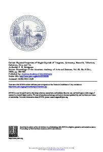
FIG. 3. The dispersion curves for M ⫽J⫽h⫽1, A⫽0.5, C ⫽4, C 1 ⫽1, and C 2 ⫽2. The three thick solid lines are the dispersion curves for the discrete model 关Eq. 共26兲 with coefficients defined by Eq. 共23兲兴. The three thin solid lines correspond to the micropolar-type approximation 关Eq. 共26兲 with coefficients defined by Eq. 共35兲兴. Open circles present the two branches of the conventional elasticity theory, Eq. 共40兲.

three thin solid lines correspond to the micropolar-type approximation 关Eq. 共26兲 with coefficients defined by Eq. 共35兲兴. Open circles present the two branches of the conventional elasticity theory, Eq. 共40兲. One can see that the two linear branches of the conventional elasticity 共open circles兲 are tangent to the acoustic branches for the discrete model 共thick solid lines兲 at k x ⫽0. The conventional elasticity does not describe the optic vibrations of the discrete model. The micropolar elasticity 共thin solid lines兲 gives a good approximation for all three branches of the discrete model in the range of k⬍ ␲ /4h. In Fig. 4 we show the same as in Fig. 3 but instead of C⫽4 we put C⫽40 in order to suppress the rotations of particles. In this case the optic branch goes up and the two continuum models 共thin solid lines and open circles兲 give almost the same approximations of the acoustic branches of the discrete model 共thick solid lines兲. One can see from Figs. 3 and 4 that the continuum approximations derived for the discrete model give an excellent approximation in the range of the long waves and the accuracy is not good for the short waves. This is a usual problem for the continuum models of structural media. When deriving the continuum analog to the discrete equations, we use the Taylor expansion, and the influence of high-order gradient terms is small for long waves but it is not small for a wavelength comparable with the size of a periodicity cell. To im-

FIG. 4. Same as in Fig. 3 but instead of C⫽4 we put C⫽40 in order to suppress the rotations of particles.

prove the approximation in the short-wave range one can take into account the fourth-order terms in the Taylor expansion. An alternative approach is the so-called many-field approximation when one uses more than one continuum field for the description of the generalized displacements. This approach was successfully used in Ref. 23 where the shortwave soliton solution for a nonlinear discrete model has been obtained. Now let us turn to the discussion of the role of rotational degrees of freedom. If particles cannot rotate 共the limit of C→⬁ or, equivalently, A→0), then ␾ (x,t) disappears from the system, Eqs. 共28兲–共30兲, and we come to the following equations of conventional elasticity for the medium without microrotations:

␳ u tt ⫽ 共 C 1 ⫹C 2 兲 u xx ⫹C 2 u y y ⫹2C 2 v xy ,

共41兲

␳ v tt ⫽C 2 v xx ⫹ 共 C 1 ⫹C 2 兲v y y ⫹2C 2 u xy .

共42兲

If the rotations of particles are not suppressed, the model, discussed in this paper, presents a micropolar medium and the equation for ␾ (x,t) must be introduced. However, even in this case, under the assumption that ␾ xx , ␾ y y , and J ␾ tt are small, we could derive Eqs. 共32兲 and 共33兲 which have the same structure as Eqs. 共41兲 and 共42兲 with coefficients redefined in order to take into account the rotations of particles. The terms ␾ xx and ␾ y y are not small in the vicinity of crystal defects like the domain wall, dislocation, free surface, or tip of a crack. They also cannot be neglected in the modulated or incommensurate phase. In all these cases micropolar-type elasticity should be used. Formally, the function ␾ (x,t) can be eliminated from Eqs. 共28兲 and 共29兲 even when ␾ xx and ␾ y y are not small and J ␾ tt is negligible but, in this case, the higher-order spatial derivatives of u and v will appear in the equations. It is well known that the incommensurate phase cannot be described without taking into account the higher-order gradient terms. We have just demonstrated that these terms can appear in the media with microscopic rotations. Thus, microscopic rotations can be responsible for the appearance of incommensurate phase in crystals. We can easily imagine the physical situation where ␾ xx and ␾ y y are small but the inertia of the rotations J ␾ tt cannot be neglected. This can happen, for example, under an applied high-frequency electric field with possible resonance with the optic branch. The coupling with the rotational mode can play an important role in the ultrasonic-wave propagation. Effects of this kind cannot be studied in the framework of conventional elasticity because the rotational optic branch is absent in this theory. Here again the equation for ␾ (x,t) must be involved in the analysis. Finally, we have shown in Sec. IV that the rotational degrees of freedom are responsible for the negative Poisson ratio in a polycrystal. As pointed out above, our model in the present form does not support an incommensurate phase. But, for example, the introduction of a third-neighbor interaction will make the vanishing of a dispersion curve inside the first Brillouin zone possible. An additional nonlinear term can make the incom-

094101-6

ELASTIC PROPERTIES OF A TWO-DIMENSIONAL . . .

PHYSICAL REVIEW B 65 094101

mensurate structure stable. Besides, the model with a nonlinearity will support solutions in the form of a domain wall or soliton and comparison with the results of Pouget and Maugin28 will become possible.

*Permanent address: Department of General Physics, Altai State Technical University, Lenin St. 46, 656099, Barnaul, Russia. 1 A. C. Eringen, Microcontinuum Field Theories: Foundations and Solids 共Springer-Verlag, New York, 1999兲; in Fracture, edited by H. Leibowitz 共Academic Press, New York, 1968兲, Vol. 2, pp. 662–729. 2 G. A. Maugin, Nonlinear Waves in Elastic Crystals 共Oxford University Press, Oxford, 1999兲. 3 R.D. Mindlin, J. Elast. 2, 217 共1972兲. 4 J. Pouget, A. As¸kar, and G.A. Maugin, Phys. Rev. B 33, 6320 共1986兲. 5 A. As¸kar, J. Phys. Chem. Solids 34, 1901 共1973兲. 6 A. As¸kar and A.S. Cakmak, Int. J. Eng. Sci. 6, 583 共1968兲. 7 A.K. Noor, Appl. Mech. Rev. 41, 285 共1988兲. 8 K.W. Wojciechowski, Phys. Lett. A 137, 60 共1989兲. 9 J. Pouget, A. As¸kar, and G.A. Maugin, Phys. Rev. B 33, 6304 共1986兲. 10 M.T. Dove et al., Phys. Rev. Lett. 78, 1070 共1997兲; I.P. Swainson and M.T. Dove, ibid. 71, 193 共1993兲. 11 D.G. Sannikov, Sov. Phys. JETP 14, 98 共1962兲; Sov. Phys. Solid State 4, 1187 共1962兲. 12 L. D. Landau and E. M. Lifshitz, Theory of Elasticity 共Pergamon Press, Oxford, 1986兲. 13 R.S. Lakes, Science 288, 1976 共2000兲. 14 D.J. Gunton and G.A. Saunders, J. Mater. Sci. 7, 1061 共1972兲. 15 R.H. Baughman, J.M. Shacklette, A.A. Zakhidov, and S.

ACKNOWLEDGMENTS

One of the authors 共S.V.D.兲 wishes to thank the Japan Society for the Promotion of Science for financial support.

Stafstrom, Nature 共London兲 392, 362 共1998兲. R.S. Lakes, Science 235, 1038 共1987兲. 17 R.S. Lakes, Trans. ASME, J. Appl. Mech. 115, 696 共1993兲. 18 M.B. Smirnov and A.P. Mirgorodsky, Phys. Rev. Lett. 78, 2413 共1997兲. 19 U. Scha¨rer and P. Wachter, Solid State Commun. 96, 497 共1995兲. 20 D.J. Bergman, Phys. Rev. B 33, 2013 共1986兲. 21 S.V. Dmitriev, T. Shigenari, and K. Abe, J. Phys. Soc. Jpn. 70, 1431 共2001兲. 22 S.V. Dmitriev, K. Abe, and T. Shigenari, J. Phys. Soc. Jpn. 65, 3938 共1996兲. 23 S.V. Dmitriev, T. Shigenari, A.A. Vasiliev, and K. Abe, Phys. Rev. B 55, 8155 共1997兲. 24 S.V. Dmitriev, K. Abe, and T. Shigenari, Physica D 147, 122 共2000兲. 25 Y. Ishibashi and M. Iwata, J. Phys. Soc. Jpn. 69, 2702 共2000兲. 26 J.J. De Yoreo, T.A. Land, and J.D. Lee, Phys. Rev. Lett. 78, 4462 共1997兲; Y.N. Huang et al., Phys. Rev. B 55, 16 159 共1997兲; S.G.C. Moreira, F.E.A. Melo, and J.M. Filho, ibid. 54, 6027 共1996兲; R. Blinc and B. Zeks, Adv. Phys. 21, 693 共1972兲. 27 Landolt Bernstein data book III/1, Elastic, Piezoelectric and Related Constants of Crystals, edited by K.-H. Hellwege, LandoltBo¨rnstein, New Series 共Springer-Verlag, Berlin, 1966兲, p. 56; ibid. book III/2, p. 53. 28 J. Pouget and G.A. Maugin, J. Elast. 22, 135 共1989兲; 22, 157 共1989兲. 16

094101-7