Modeling of Roughness Effects on Electromagnetic Waves Propagation above Sea Surface Using 3D Parabolic Equation. Othmane Benhmammouch, Natacha Caouren, Ali Khenchaf
[email protected],
[email protected],
[email protected] Laboratoire E3I2 (EA-3876) ENSIETA (Ecole Nationale Supérieure des Ingénieurs des Etudes et Techniques de l’Armement) 2 rue François Verny, 29806 Brest cedex.
2. Abstract This paper deals with effects of sea surface roughness on electromagnetic waves propagation in a threedimensional domain. The 3D Parabolic Equation method is used to solve the wave equation. A new approach is presented to model the propagation above rough sea surface. Numerical results of electromagnetic waves propagation are presented to highlight the sea surface roughness influence. Index Terms— Tropospheric propagation, 3D parabolic equation, Split Step Fourier, sea spectrum, rough sea surface. 1.
INTRODUCTION
In coastal surveillance domain, radar performances prediction is important notably for radar system parameterization. Numerous methods are able to predict the electromagnetic waves propagation; they require a good understanding of various interaction phenomena between wave and propagation medium. The prediction strongly depends on good propagation domain characterizations: marine atmosphere (troposphere with or without tropospheric ducts) and sea surface. This paper deals with works on radar links in a threedimensional marine environment. The prediction of radar performances is related to the electromagnetic waves propagation modeling in maritime environment [1]. The troposphere propagation modeling requires a good consideration of meteorological parameters and a realistic characterization of wave interaction with the sea surface (taking into account of reflection and surface roughness). This article will focus on three sides. The first one is the modeling of electromagnetic waves propagation, using 3D parabolic wave equation and a Split Step Fourier algorithm [2]. The second one consists on presentation of a hybridized method for a better taking into account of sea surface roughness in wave propagation [3][4]. Finally some simulation results are presented and analyzed, for different configurations and different sea states, in a threedimensional propagation domain.
ELECTROMAGNETIC PROPAGATION MODELLING USING 3D PARABOLIC EQUATION
To model electromagnetic waves propagation in a three-dimensional domain we use the 3D Parabolic wave equation technique [2][5], more easy to solve and less burdensome in terms of boundary and mesh conditions. The original idea of using 3D parabolic equation in electromagnetic propagation and scattering was introduced by A. Zaporozhets and M. Levy [6][7]. R. Janaswamy proposed a mixed-potential split step Fourier method to calculate the path loss in an urban environment [2]. In this paper, 3D parabolic equation is used to give a prediction of path loss in a maritime environment, introducing the roughness sea surface effects on propagation phenomena. Fig.1 represents the geometrical description of 3D parabolic equation configuration used in this paper.
Fig.1: Geometrical configuration for 3D parabolic equation.
The source is placed in an initial plane P 1 , we are interested by the calculation of electromagnetic field propagated in successive planes P 2 , P 3 … (parallel and equidistant) using an iterative algorithm. The backscattered field is neglected so we consider a forward propagation. The parabolic equation technique introduces hypotheses on the conventional elliptical equations of
propagation to obtain a parabolic equation given by the following formula: 1 ∂ 2ψ ∂ 2ψ ∂ψ −j + 2k ∂y 2 ∂z 2 ∂x
k − j m 2 + 1 ψ = 0 2
(
)
(1)
k : the wave vector ψ : the electric or magnetic field m = n + z R : the modified refractivity index. n : the refractivity index. R : the earth radius in meter. To solve this equation we use a Split Step Fourier method [1][8][9]: jk ∆x ( m +1) − j ∆x (k +k ) ψ (x + ∆x, y, z ) = e 2 FT −1 e 2 k FT {ψ ( x, y, z )} (2) 2
2 y
2 z
FT : the Fourier Transform. FT-1 : the inverse Fourier Transform. k y : the projection of wave vector in y plane. k z : the projection of wave vector in z plane. Δx : the Split Step Fourier algorithm step. For a realistic modeling of 3D electromagnetic waves propagation same boundary conditions are required (interaction with sea surface and radiation conditions towards infinity). In this work, we use impedance boundary conditions to represent the loss induced by the sea surface [2][5]. To satisfy Sommerfeld radiation conditions, an absorption area is added beyond a maximum distance from the source [10][11]. In this area the field is multiplied by an attenuation function (quick decrease towards zero) (Plane P n Fig.1). 3.
INTRODUCTION OF SEA SURFACE ROUGHNESS IN PROPAGATION
Usually, in electromagnetic waves propagation modeling [8][9], we use perfectly reflecting and flat sea surface, this approach doesn’t allow the introduction of sea surface roughness effects on propagation. A more realistic model of electromagnetic waves propagation must take into account these effects. An existing method [12][13] consists to multiply the Fresnel reflection coefficients by a roughness parameter which depends on: the wind speed, the roughness parameter of Rayleigh and the probability distribution of surface’s heights. This method doesn't model the influence of the surface’s geometry in propagation, since the sea surface is considered as flat. In order to introduce the effects of sea surface geometry, in electromagnetic waves propagation, we developed a new method which is the result of a combination of two approaches. The sea surface can be considered as the superposition of two surfaces with tow scales of roughness (a large roughness surface and a small roughness surface). The main idea of our approach is to model each type of roughness differently. To make those, we divide the sea spectrum in two parts: the first represents the large roughness and the second
the small roughness. The first part of spectrum (large roughness) is used to generate a sea surface and the second part is used to calculate a new roughness parameter which models only small roughness. This modified roughness parameter is introduced in Fresnel’s reflection coefficient and the electromagnetic wave is propagated above rough sea surface using the method given by Mac Arthur and Bebbington [14]. 3.1. Sea surface generation: Sea surface spectrums represent a statistical description of wind-generated surface waves. In scientific literature we find several models (Bjerkaas and Riedel [15], Donelan and Pierson [16], Elfouhaily [17] ...). The spectrum is a 2D function written as a product of two components:
S
( K ,φ ) =
1 K
S (K ) S (K , φ ) 1d
dir
(3)
S 1d represents the omnidirectional wave height spectrum and S dir the spread function. K=[K x ,Ky] is the ocean wave vector. For the omnidirectional wave height spectrum S 1d we use the Elfouhaily model. The Elfouhaily spectrum seems to be in agreement with reality and the simplest in its analytic form. For the spread function S dir the model proposed by Longuet-Higgins [18]: 2 s − 1 Γ(s + 1) ϕ − ϕ0 S dir (K ) = cos 2 (4) 2 π Γ(2 s + 1) s ≥ 2 is an integer parameter, Γ is Euler’s Gamma function, φ 0 is the direction of the wind and φ the wave’s propagation direction. The sea surface generation (Fig.2) is based on a stochastic process, with arbitrarily specified correlation properties calculated using S(K) [19][20]. Due to the discretization steps Δx and Δy, we can’t represent all levels of sea surface roughness. The discretization steps ΔK x and ΔK y are given by: 2π ; 2π ∆K x =
N x ∆x
∆K y =
N y ∆y
(5)
N x and N y the numbers of points in the range and horizontal discretization. Using ΔK x and ΔKy we can calculate K xmax and K ymax , the maximal wave numbers that can be represented in the generated surface. This wave number represents also the cutting point of the sea surface spectrum. All the wave numbers above K xmax and K ymax are not taken into account in the sea surface generation. The sea surface generation method allows us to introduce, in the modeling of electromagnetic waves propagation, the effects of surface roughness. But the limitation imposed by the horizontal discretization penalizes this approach. This led us to find a method to take into account the effects of small roughness. This method consists on an introduction of a modified roughness coefficient which will take into account only the small roughness.
3.2. Modified roughness coefficient We can’t ignore the effects of small roughness on the electromagnetic waves propagation. We model these effects using a modified roughness coefficient. For our work we adapt the Miller et al. roughness parameter to introduce only the small roughness effects.
Fig.2: generated sea surface for a sea state of 5 in Beaufort scale (10ms-1).
The standard deviation of the wave elevation h s used in the calculation of roughness parameter is replaced by h c the standard deviation of small roughness (K > K max ) which is calculated using Elfouhaily sea spectrum: ∞
hc =
∫ S1d ( K )dK
5.
CONCLUSION AND FUTURE OUTLOOKS
(6)
K max
3.3. Propagation above generated rough surface Once the sea surface created and the roughness coefficient introduced in Fresnel’s reflection coefficient, the electromagnetic field is propagated above the sea surface using the method exposed by Mac Arthur and Bebbington. In this method the sea surface is represented by a staircase surface, the part of fields which is on the obstacle (in our case the sea) is set at zero; the field at the surface is calculated and then propagated using the SSF algorithm. In our approach we have hybridized two methods; the first one is the surface generation (for large roughness modeling) and the second is the modified roughness parameter (for small roughness modeling). With this concept, we have involved all roughness scales in the electromagnetic waves propagation simulations. 4.
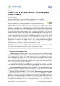
75m height and 150m width. The following numerical results represent the one-way propagation loss computed in X-band (9 GHz). The sea state is 5 in Beaufort scale (10ms-1). The result is a 3D matrix; we present here a vertical cut through the source and a horizontal cut through the source. To visualize the effect of generated sea surface roughness on radar coverage, we present here averages of several simulation of propagation for several sea surfaces generated randomly. These results are given for a flat and rough surface. The aim is to highlight the effects of surface roughness on propagation losses and therefore on the radar coverage. Indeed we can see these effects on results Fig.3-b and Fig.3-d. By comparing the results (Fig.3-a and Fig.3-b), we note that the number and shape of the interference lobes change. We also note that the geometry of the generated surface, taken into account in the phenomenon of propagation, increases path loss. But in horizontal cuts (Fig.3-c and Fig.3-d) the sea surface roughness generated better reparation of the propagated energy. In Fig.3-c (between 15.5Km and 17Km) the presence of an interference lobe generates an area with large loss (between 160 and 170 dB). Through the diffraction caused by the roughness of the surface, this area is better lit and the average losses are around 140dB.
NUMERICAL RESULTS
In this section the numerical results are computed for different sea states in X-band. The results are used to show the sea surface roughness influence in electromagnetic waves propagation in a threedimensional domain. We consider a source placed at 20m height from the sea surface, the propagation domain is 24Km length and
The main purpose of this paper is to introduce the sea surface roughness in the simulations of electromagnetic waves propagation in a threedimensional marine environment. For this we introduced an original method based on generation of sea surfaces. An evolution of our works will be the introduction of different atmospheric conditions and notably the presence of three-dimensional tropospheric ducts. 6.
REFERENCES
[1] M. F. Levy, “Parabolic Equation Methods for Electromagnetic Wave Propagation”, IEE Electromagnetic Waves Series, April 2000. [2] R. Janaswamy, "Path loss predictions in the presence of buildings on flat terrain: a 3-D vector parabolic equation approach", IEEE Transactions on Antennas and Propagation, Volume: 51, Issue: 8, pp 1716- 1728, Aug. 2003. [3] O. Benhmammouch, A. Khenchaf, N. Caouren, “Electromagnetic Waves Propagation above Rough Sea Surface Application to Evaporation Ducts”, IGARSS 2008, Boston July 2008. [4] O. Benhmammouch, L. Vaitilingom, A. Khenchaf, N. Caouren, “Electromagnetic Waves Propagation above Rough Surface: Application to Natural Surfaces”, PIERS 2008, Cambridge, July 2008. [5] R. Janaswamy, “Radiowave Propagation & Smart Antennas for Wireless Communications”, Kluwer Academic Publishers, 2000. [6] A. A. Zaporozhets and M. F. Levy, “Bistatic RCS calculations with the vector parabolic equation method,”
IEEE Trans. Antennas Propagat., vol. 47, no. 11, pp. 1688–1696, Nov. 1999. [7] A. A. Zaporozhets and M. F. Levy, “Radar cross section calculation with marching methods,” Electron. Lett., vol. 34, no. 20, pp. 1971–1972, 1998. [8] G.D. Dockery, “Modeling electromagnetic wave propagation in the troposphere using the parabolic equation”, IEEE Trans., AP-36, pp. 1464-1470, 1988. [9] H. W. Ko, J. W. Sari, M. E. Thomas, P. J. Herchenroeder and P. J. Martone, “Anomalous propagation and radar coverage through inhomogeneous atmospheres,” AGARD Conf. Proc., Vol. 346, pp. 1–14, 1984. [10] M. Grábner, and V. Kvičera, “Clear-air propagation modelling using parabolic equation method”, Radioengineering 12, pp. 50-54, 2003. [11] K. H. Craig and M. F. Levy, “Parabolic equation modelling of the effect of multipath and ducting on radar systems”, IEE Proc. F, Vol. 138, N° 2, pp. 153162, April 1991. [12] W. S. Ament, “Toward a theory of reflection by a rough surface”, Proc. IRE, Vol. 41, pp. 142-146, 1953. [13] A. R. Miller, R. M. Brown and E. Vegh, “New derivation for the rough surface reflection coefficient and for the distribution of sea-wave elevations”, IEE Proc. IRE, Vol. 131,Part H, pp. 114-116, 1984. [14] R. J. Mac Arthur and D. H. O. Bebbington, “Diffraction over simple terrain obstacles by the method of parabolic equation”, ICAP91, N° 333, pp. 2.824-2.827, October 1992. [15] A. W. Bjerkaas, and F. W. Riedel, “Proposed model for the elevation spectrum of a wind-roughened sea surface”, Tech. Rep. ALP-GT1328-I-31, 31 pp., 1979. [16] M. A. Donelan, and W. J. P. Pierson, “Radar scattering and equilibrium ranges in wind-generated waves with application to scatterometry”, J. Geophys. Res., 92, pp 4971-5029, 1989. [17] T. Elfouhaily, B. Chapron, K. Katsaros and D. Vandemark, “A unified directional spectrum for long and short wind-driven waves”, Oceans 97, Vol. 102, No. C7, p. 15,781-15,796, July 1997. [18] M. S. Longuet-Higgins et al., Ocean Wave Spectra. Prentice-Hall, Inc., 1963, ch. Observations of the Directional Spectrum of Sea Waves Using the Motions of a Floating Buoy, pp. 111–136. [19] A. Arnold-Bos, A. Khenchaf, & A. Martin, "Bistatic radar imaging of the marine environment. Part 1: theoretical background", IEEE Transactions on Geoscience and Remote Sensing, Special Issue on Synthetic Aperture Radar, Vol 45(11), November 2007. [20] A. Arnold-Bos, A. Khenchaf, & A. Martin, "Bistatic radar imaging of the marine environment. Part 2: simulation and results analysis", IEEE Transactions on Geoscience and Remote Sensing, Special Issue on Synthetic Aperture Radar, Vol 45(11), November 2007.
(a)
(b)
(c)
(d) Fig.3: One way path loss in X-band, (a) (b) Vertical and horizontal cut for a flat sea surface, (c)(d) Vertical and horizontal cut for a generated sea surface (state 5 in Beaufort scale 10ms-1).