Abstract. The electron gun plays an important role concerning klystron performance, especially for X-band klystrons with a small drift-tube diameter. This paper ...
ELECTRON GUN SIMULATION USING MAGIC S. Michizono, H.Tsutsui, S. Matsumoto, Y. H. Chin and S. Fukuda High Energy Accelerator Research Organization (KEK), Tsukuba, Ibaraki 305-0801 Japan Abstract The electron gun plays an important role concerning klystron performance, especially for X-band klystrons with a small drift-tube diameter. This paper describes a new method for an electron-gun simulation by using MAGIC. MAGIC solves the Maxwell equations in the presence of charged particles on a time-domain. The results simulated by MAGIC are compared with those by EGUN and measured values. It reveals that the perveance is almost the same as the measured values, and that the current-density distribution and beam angle are almost the same as those of EGUN. Although it takes half days to simulate the gun, the simulation has the potential that a single code can enable one to simulate the whole structure of a klystron.
1 INTRODUCTION It is important to design the electron gun precisely when we design klystrons. In a future linear collider, such as Japan Linear Collider (JLC) and SLAC NLC, highpower klystrons at the X-band (11.424 GHz) will be used. In these klystrons, the beam (>350A) should be compressed to around a radius of 3 mm and the areaconvergence ratio of the beam should be more than 100. In order to simulate a whole structure of a klystron precisely by a single code, we started to use a 2.5D particle-in-cell (PIC) program, called “MAGIC”[1], which is used in plasma-physics problems. In MAGIC, neither a port approximation nor an equivalent-circuit model is used, and only the geometry of the structure is necessary to be input. By using a general program (“MAGIC”), one can modify and develop a simulation system by oneself, even if a new idea for klystrons occurs. In the klystron, the gun and all rf components are electromagnetically divided from each other, and the simulation is executed at three parts (gun, buncher and output) [2-4]. We report on the results of some klystronguns (S- and X-band) simulated by MAGIC.
Since the electrons emitted due to the electric-field strength on every grid of the cathode, a careful configuration of the cathode surface is important to avoid edge emission. In order to construct the boundary condition easily, we made a program similar to the boundary-definition-program POLYGON [5] used for EGUN [6]. Figure 1 shows a schematic of the electrongun boundary. The grid dimensions, such as ∆r and ∆z, must be defined in the program. Since the grids should be located on the drift tube wall, the number of grids existing in the r-direction of the drift tube is necessary as an input. There are restrictions in the number of grids (rand z-directions and total numbers), and the grid sizes depend on the geometry size. It is possible to simulate a “small area” (divided by “GAP” line in Figure 1) after the simulation of a “large area” (total area of Figure 1). In a small-area simulation, the electric-field (Ez) distribution on “GAP” obtained by a “large-area” simulation is used for the voltage input. Although a “small-area” simulation is possible only when the “GAP” can be treated as a Neumann boundary, this is convenient to reduce the number of cells or to make a precise simulation. By using this boundary program, it becomes easy to compare the data obtained by EGUN.
2.2 Time step of “rough” and “fine” simulation The data of particles and electromagnetic fields are repeatedly imported at the next buncher and output region, and the time step should be a divisor of the period of the operation frequency. When we simulate the entire structure of a klystron, it is selected as 0.24315 ps (“fine” simulation) in an X-band klystron (XB-72k [7]), which corresponds to 1/360 of the period (1 degree). The default time step with 0.5 mm grids is about 0.8 ps, which reduces the simulation time (“rough” simulation). This is convenient when we simulate only the electron-gun
"large area" "inlet"
2 BOUNDARY PREPARATION
GAP
2.1 Spatial geometry of “large” and “small” area
"small area"
In MAGIC, arbitrary rectangular grids are used and the spatial grid is the primary determinant of accuracy. It is especially necessary to define fine grids in a spherical cathode and the small aperture of the drift tube radius.
z _outp ort
Figure 1 Schematic of electron gun giometry.
493
region. Both “rough” and “fine” simulations gave the same results in the gun region.
2.3 Magnetic fields The magnetic fields used for electron-beam convergence can be introduced from the output of the LANL POISSON/PANDIRA codes [8].
2.4 Cathode voltage In MAGIC, the voltage is applied at “inlet” in Figure 1 is a “large-area” simulation and at “GAP” in Figure 1 in a “small-area” simulation. Since MAGIC is a time-domain code, the applied voltage should gradually be increased so as to avoid any numerical oscillations: we set 0.8 ns for the rise time.
Figure 2 Particle trajectories of XB-72k with “smallarea” and “fine” time step. The applied voltage and beam current are 550 kV and 490 A respectively.
3 PERFORMANCE OF MAGIC 3.1 Execution procedure The execution of a MAGIC simulation is done as follows: (1) “Large-area” simulation with a “rough” time step If the “GAP” (in Figure 1) can be treated as a Neumann boundary, then (2) Input the electric-field distribution on “GAP” (3) Make a “small-area” simulation with a “fine” time step After the simulation, the particle and field data can be exported to the next buncher and the output region of the klystron.
3.2 Output data Since MAGIC is a general code for plasma problems, we can specify the output of the simulations. (1) A phase plot (particle trajectory) is obtained by MAGIC. Figure 2 shows the trajectories of XB-72k with an applied voltage
of 550 kV. Due to a careful grid configuration, edge emission is not observed. (2) The transition of the beam current and voltage between a wehnelt and an anode are monitored in order to evaluate the machine time necessary to be stable. A simulation of the XB-72K with 0.5 mm grids requires 15 ns (about 60,000 time steps with “fine” simulation) to be stable. By using exported particle data, (3) the current density distribution and (4) beam angle (vR/vz) are also obtained. We can compare results (1), (3) and (4) with those of EGUN. Figure 3 shows the current-density profile of XB72K by MAGIC together with that obtained by EGUN. The results obtained by MAGIC agree well with that by EGUN. Figure 4 shows the radial distribution of the beam angle obtaiend by MAGIC and by EGUN. Since the position of the beam waist was different between EGUN and MAGIC, probably caused by a difference in the total beam current (450 A in EGUN and 490 A in MAGIC), the beam angle by MAGIC is about half that obtained by EGUN.
45.0 40.0
EGUN
35.0 30.0
ALFA [mRAD]
2
Current density [A/mm ]
50.0
MAGIC
25.0 20.0 15.0 10.0 5.0 0.0 0.0
1.0
2.0 3.0 R [mm]
10 0 -10 -20 -30 -40 -50 -60 -70 -80 -90 0.0
EGUN MAGIC
1.0
2.0 R [mm]
3.0
4.0
4.0 Figure 4 Electron-beam angle (vr/vz) of the electron gun (XB-72k) at 175 mm in the Z-direction. About half the value of MAGIC is due to the difference in the beam oscillation position (see Figure 5).
Figure 3 Current-density distribution of the electron gun (XB-72k) at 175 mm in the Zdirection.
494
(b)
(a)
Figure 5 Beam trajectories obtained by MAGIC (a) and EGUN (b) from z=175 mm to 500 mm of XB-72k. The oscillation is almost the same, but the phase is different, probably due to a difference in the total current.
3.3 Diode simulation By importing particle data from electron-gun region, we can simulate the drift-tube region. Figure 5 shows the particle trajectories of the diode together with that by EGUN. The trajectories obtained by MAGIC are almost the same as those obtained by EGUN.
3.4 Performance and machine time The performance and machine time are summarized in Table.1. Simulations by MAGIC are carried out not only for an X-band klystron, but also for the S-band klystrons used in the KEK(PV3030A2)[9] and SLAC(5045)[10,11]. The perveances are almost the same as the measured values and 5-10% larger than those obtained by EGUN. The machine time depends on the grid size and time step; it takes about 15 hours to simulate “15 ns” with a “small-area” and “fine” time step by PentiumPro200MHz PC. Now, the pentiumII-300MHz PC is used, which reduces the simulation time by half. Table 1 Performance of a MAGIC simulation. Klystron PV3030A2 5045 XB-72K Frequency 2,856 MHz 2,856 MHz 11,424 MHz Voltage 300 kV 315 kV 550 kV Experimental µperveance 2.05 2.0 1.2 EGUN Grid size 0.5 mm 0.5 mm 0.5 mm µperveance 1.89 1.78 1.10 machine-time* 2 min. 2 min. 6 min. MAGIC Grid size 0.5 mm 0.5 mm 0.5 mm Time step 0.9726 ps 0.9726 ps 0.24315 ps µperveance 2.03 1.99 1.19 machine-time* 5 hours 5 hours 15 hours *The time simulated by PentiumPro200MHz PC.
4 SUMMARY An electron-gun simulation was successfully carried out by MAGIC. A boundary-formation program was
developed which makes it convenient for comparisons with EGUN. (1) The particle trajectories, (2) transitions of the voltage and beam current, (3) current-density distribution, and (4) beam angle were obtained; the results agree well with those obtained by EGUN. The obtained perveances were almost the same as the measured values for the S- and X-band klystrons. Although it takes more than a half day to simulate with a fine time-step used for a whole-structure calculation, the machine time can be reduced by using a faster PC. Since the whole-structure simulation reveals good agreements with the measured values, this simulation method is useful for the final stage of klystron design.
5 REFERENCES [1] Mission Research Corporation, Virginia, USA. [2] Y.H.Chin, “Computational Modeling of Klystrons”, this conference. [3] S.Matsumoto et al., “Simulation study of the bunching section of X-band klystrons”, this conference. [4] H.Tsutsui et al., “X-band klystron output cavity simulation”, this conference. [5] R. Becker, “Easy boundary definition for EGUN”, Nucl. Inst. Meth. B42,162-164 (1989). [6] W.B.Herrmannsfeldt, “Developments in electron gun simulation”, SLAC-PUB-6498 (1994). [7] J.Odagiri et al., “FCI simulation on 100 MW class th klystron at X-band”, Proceedings of the 17 International Linac Conference, Tsukuba, Japan, 469-471(1994). [8] J.H.Billen and L.M.Young, “POISSON SUPERFISH”, LA-UR-96-1834(1997). [9] S.Fukuda et al., ”Design and evaluation of a compact 50-MW rf source of the PF linac for KEKB project”, Nucl. Instr. Meth. A363,83-89 (1995). [10] T.G.Lee et al., ”A fifty megawatt klystron for the stanford linear collider”, SLAC-PUB-3214 (1983). [11] M.A.Allen et al., “Performance of the SLAC linear collider klystrons”, SLAC-PUB-4262 (1987).
495