Embedding Spatial Context Information into Inverted File for Large-Scale Image Retrieval Zhen Liu † , Houqiang Li † , Wengang Zhou ‡ , Qi Tian ‡ †
University of Science and Technology of China, Hefei 230027, P. R. China ‡ University of Texas at San Antonio, Texas, TX 78249
[email protected];
[email protected];
[email protected];
[email protected] ABSTRACT
1.
One most popular approach for large-scale content-based image retrieval is based on the Bag-of-Visual-Words model. Since the spatial context among local features is very important for visual content identification, many approaches index local features’ geometric clues, such as location, scale and orientation for post-verification. To obtain consistent accuracy performance, the amount of top ranked images that post-verification approach needs to process is proportional to the image database size. When the database is very large, the verified images will be too many to be processed in real-time response. To address this issue, in this paper, we explore two approaches to embed spatial context information into the inverted file. The first one is to build a spatial relationship dictionary embedded with spatial context among local features, which we call one-one spatial relationship method. The second one is to generate a spatial context binary signature for each feature, which we call one-multiple spatial relationship method. Then we build an inverted file with spatial information between local features. The geometric verification is implicitly achieved while traversing the inverted file. Experimental results on benchmark Holidays dataset demonstrate the efficiency of the proposed algorithm.
In recent years, content-based image search has attracted more and more attention in computer vision and multimedia community owing to its great potential in both industry applications and research problems [18] [17] [1] [23] [21] [22]. Most approaches rely on the Bag-of-Visual-Words (BoW) model [18]. Generally, an image is represented by a set of local features. Those local features are extracted by describing local patches around key points. Key points are usually obtained by invariant detectors, such as Difference of Gaussian (DoG) [13], Harris affine detector [15], and MSER [14], etc. Then around a key point, a local patch is described into a local feature, such as SIFT [13]. Local features are usually of high dimension. To achieve a compact representation, a visual dictionary is defined and then local features can be quantized to visual words. The visual dictionary can be constructed off-line by unsupervised clustering algorithm, typically k-means [18], hierarchical k-means (HKM) [16] or approximate k-means (AKM) [17]. Consequently, an image is represented by a set of visual words. Further, scalable indexing techniques are leveraged from information retrieval. Typically, the inverted file structure, which has been successfully applied in textual information retrieval, is leveraged to index large-scale image database. However, with the ignorance of spatial context among local features, the standard Bag-of-Visual-Words model suffers from limited accuracy [17]. To tackle the problem, many local or global verification methods, such as RANSAC [5] [2], weak geometric consistency [9] [11], geometric coding [25] [26], are proposed to check the geometric consistency among matched local features. RANSAC is one of the most popular methods for global post-verification. Since RANSAC is involved with many times of affine estimation for random sampled matching pairs, it is very time-consuming. By encoding local spatial informatin in stable regions, for example MSER region in [20], ”Bundled features” can address the problem to some extent. But, it is still time consuming since the spatial verification between two bundled features is carried out during the retrieval process [21]. In contrast, geometric coding [25] is much efficient, but still unavoidably incurs additional time cost for spatial verification. What’s more, such time cost is proportional to the size of image database. Although, on one million image database, the average query time is very short, say less than 100 milliseconds for 400 features in one image, it is still far from acceptable when the database size scales to 100 million or even billion scale. However, if we embed the spatial context information into the indexing structure, no post-verification will be need-
Categories and Subject Descriptors I.2.10 [Vision and Scene Understanding]: VISIONS
General Terms Algorithms, Experimentation, Verification
Keywords large-scale image retrieval, SIFT, spatial context , spatial relationship dictionary, one-one relationship, one-multiple relationship, feature tuple, spatial context binary signature
Permission to make digital or hard copies of all or part of this work for personal or classroom use is granted without fee provided that copies are not made or distributed for profit or commercial advantage and that copies bear this notice and the full citation on the first page. To copy otherwise, to republish, to post on servers or to redistribute to lists, requires prior specific permission and/or a fee. MM’12, October 29–November 2, 2012, Nara, Japan. Copyright 2012 ACM 978-1-4503-1089-5/12/10 ...$15.00.
Area Chair: Gang Hua
199
INTRODUCTION
Figure 1: An example of some random selected feature tuples. The green arrow line means the dominate orientation of local feature and the red two pixel width line represents the pair of local features consisting of one feature tuple.
Figure 2: An example of spatial context of 5 random selected features. The green line means the dominate orientation of local feature and the red two pixel width circle represents the range of meaningful feature surrounding of the center feature. What’s more, the circle is parted into three parts by the blue two pixel width radius.
ed. Motivated by this, our target is to design an algorithm that can record the spatial context information into the inverted file, because the indexing stage can be done off-line. And in the online retrieval stage, we just need to process the spatial context information of the query image. In this paper, we explore embedding the spatial information between local features into the inverted file. It has been revealed that two order spatial structure between single features is much more important than other higher order spatial structure [6] [12] [24]. Therefore, we first propose an one-one relationship approach to record feature tuples into the inverted file instead of single feature. The feature tuple consists of a pair of single features and their spatial relationship, as illustrated in Fig. 1. In Fig. 1, the green arrow line denotes the dominate orientation of local feature and the red two pixel width line represents the pair of features consisting of one feature tuple. As for the high resolution image, a lot of local features can be extracted by the interest feature detector, such as 3000 features per image for Holidays [8]. The available memory limits the number of feature tuples that can be recorded into the inverted file. Thus the amount of spatial structure recorded into the inverted file is limited. To record spatial structure information as much as possible with the limited memory, we propose the one-multiple relationship approach. In the one-multiple relationship approach, for each single feature, its surrounding features are clustered into different groups based on their spatial relationship with it. A toy example is illustrated in Fig. 2. The center feature of the red circle is the feature whose spatial context need to be described. And the other features that locate inside the circle are thought to be meaningful neighbors of the center feature. The circle is divided into three parts by the blue radius line which is determined by the dominate orientation of the center feature. Those surrounding features that locate in the same part of the circle belong to the same group. With the help of these grouped surrounding features, we generate a b bits binary signature to describe the center feature’s spatial context. Actually, for each feature in the image, we calculate its spatial con-
text binary signature in the same way. In the retrieval stage, we compute the Hamming distance with XOR operation between the spatial context binary signature of two features that are quantized to the same visual word. And with the help of the computed Hamming distance, some false matches are filtered out. Note that our spatial context binary signature is different from the Hamming Embedding approach [9]. Our method is to model spatial structure between single features of an image while Hamming Embedding is a quantization approach. Thus when traversing the inverted file, we conduct the geometric verification implicitly, which is much more scalable than the post-verification method [5] [17] [25] and make it more suitable for large-scale image search. The main contribution of this paper is summarized as follows: • We embed the spatial information between local features into the inverted file. • We build a spatial relationship dictionary to quantize the spatial relationship between local features. • We produce spatial context binary signature for each local feature to do geometric verification. The rest of the paper is organized as follows. In Section 2, related works are reviewed. In Section 3, we introduce our scheme of embedding the spatial information into the inverted index file by building a spatial relationship dictionary. In Section 4, we introduce our approach to generate spatial context binary signature for each feature. In Section 5, We present experimental results and make some discussions. Finally, we conclude the paper in Section 6.
2.
RELATED WORK
In the past decade, with the introduction of local features, many image retrieval approaches are proposed based on the popular Bag-of-Visual-Words model. With local features,
200
such as SIFT, quantized to visual words, images are compactly represented by a bag of visual words. Further, by indexing images with the inverted file structure, scalability of image search is achieved. The spatial context among local features plays an important role in visual content identification. Many approaches [18] [17] [5] [1] [26] [24] [3] explore the spatial context information in images to improve retrieval precision. These approaches can be summarized into pre-verification or postverification approaches. Some representative approaches of each category are discussed below. The motivation of pre-verification approaches is to express the spatial context of local features into the image representation. In [19], the statistics in the local neighborhood of invariant features is used as its spatial context to enhance the discriminative power of visual word. The statistics contains the number of neighborhood features, the average characteristic scale difference and the average dominate orientation difference between each local feature and its neighborhood features. The feature matches are weighted by the difference of these statistics. The shortage of this method [19] is that it abandons the information of neighborhood features’ descriptors. [1] project local features of an image along different directions to yield ordered spatial-bag-of-features for image search. Then some heuristic operations are exploited to achieve invariance in translation, rotation and scale changes. In [24], geometry-preserving visual phrase is proposed to describe the spatial context of local features, including both co-occurrences and the long-range spatial layouts of visual words. Actually, it transfers the geometric verification from the post-verification stage to the retrieval stage using Hough transform. The post-verification approaches aim to filter out false matches by imposing spatial consistency. Some approaches are focused on local spatial consistency. The local spatial consistency of some spatial nearest neighbors is used in [18] to suppress false visual word matches. ”Bundled features” [20] weights the traditional tf − idf [18] [16] by similarity between feature bundles. The local spatial consistency is measured by projecting feature positions along horizontal and vertical directions in local MSER regions. However bundling feature method is time consuming because the spatial verification between bundles is carried out during the retrieval process. Geometric min-hashing [3] constructs repeatable hash keys with loose local geometric information to obtain more discriminative local description. To capture spatial relationships of all features in the entire image, global geometric verification approaches such as WGC (weak geometric consistency) [9] [11], RANSAC [17] [5] are often adopted. Weak geometric consistency use a weaker global geometric model. The matches with the dominate relative scale difference and the relative orientation difference are thought to be true matches and other matches are filtered out. What’s more, a priori knowledge is added into the weak geometric consistency model to improve the retrieval accuracy one step further based on human shot tendency. RANSAC-based image re-ranking achieves the state-of-art result in terms of retrieval accuracy [17]. But, RANSAC has to randomly sample many subsets of matching pairs and perform affine estimation for each subset to obtain the optimal transformation. Although RANSAC can greatly improve retrieval performance, it is computationally expensive. In practice, it is usually applied to the subset of
the top-ranked candidate images to ensure efficiency, which may not benefit the recall performance in large-scale image retrieval systems. The spatial coding approach [26] and geometric coding approach [25] are another global geometric verification methods proposed to remove false matches based on maps, which are generated by checking the relative locations of local features. They are much more efficient than RANSAC, but still unavoidably incur additional time cost for geometric verification. And such time cost is still proportional to the size of image database. Based on the analysis above, we propose an algorithm to embed the spatial context information into the inverted file. The time cost to obtain spatial context information is just dependent on the query image. And we do geometric verification while feature matching.
3.
ONE-ONE RELATIONSHIP
In this section, we introduce our one-one relationship approach to record the spatial context information of an image into the inverted file. First, we build feature tuples with the spatial relationship dictionary built in Section 3.1. Then, we introduce how to index and do retrieval with feature tuples in Section 3.2 and Section 3.3. Let us first introduce our notation. We extract the interest points with Hessian-Affine detector [7] and the SIFT descriptor [13] for each image. These interest points are denoted by {fi }N i=1 , in which N represents the total number of the detected interest points. Each feature fi includes the descriptor di ∈ RD , for SIFT descriptor D is 128, the location li ∈ R2 , the characteristic scale si and the dominant orientation oi .
3.1
Build Spatial Relationship Dictionary
With the information provided by interest point detector and descriptor, namely the feature location, the dominant orientation, the characteristic scale, we build a spatial relationship dictionary by image plane division, as shown in Fig. 3. For each feature fi , a reference coordinate system is built, with the location li as the origin and the orientation oi as x axis. The different plane division means different spatial relationship quantization. The spatial relationship between feature fi and fj is denoted by Rij and we create a tuple {fi , fj , Rij } to represent this concept. We take Fig. 3 (a) as an example to illustrate how to build the spatial relationship dictionary and how to quantize the feature pairs with this spatial relationship dictionary. There are two features, A and B on the image plane. For feature A, we build a coordinate system with lA as its origin and oA as its x axis. We identify each part of the image plane divided by this coordinate system with an integer number. And feature B is processed in the same way. So there is a tuple in Fig. 3 (a), {A, B, RAB } or {B, A, RBA } . The spatial relationship between A and B, namely RAB or RBA , can be easily determined by computing the angle between −→ vector AB and the dominate orientation of A, namely oA , as shown in Fig. 4. So we have the result of RAB = (1, 2) and RBA = (2, 1). Thus for each feature tuple, there are two ways to describe it. Take the feature tuple that consists of A and B as an example, it can be noted as (A, B, RAB ) or (B, A, RBA ). We just record once for each tuple, so there must be a rule to reveal which version of the feature tuple should be embedded into the inverted file. The problem
201
2
2
3
B
0
3
A
A 3
0
1
2
1
2
1 7
B
0
7
2
0
1
1
2 1
3
6
0
3
A
6
5
A 3
5
0
B
4
1 2
B
4
3
1
2
3
0
0
(b)
(a)
(a)
(b)
2
0
2
Figure 4: Illustration of how to build a relationship dictionary and how to quantize the relationship between two features with the relationship dictionary.
4
3
6 5
6
B
1
5
7
1
A0 3 7
4
gain. Note that the two visual vocabularies can be different in size. It is easy to control the maximum of the integer ID assigned to each feature tuple by adjusting the size of two visual vocabularies. The integer ID for each feature tuple can be obtained by
(c)
Figure 3: Illustration of relationship quantization between two features, A and B. (a). The plane is divided into four partitions only with the orientation information. (b) The plane is divided into eight partitions only with the orientation information. (c) The plane is divided into eight partitions with the scale information of the feature, in which the radius of the circle is linear to the feature scale.
ID = Q{(fi , fj , Rij )} (1) = Q1 (fi ) · vocSize2 · rSize + Q2 (fj ) · rSize + Rij where ID means the integer ID for the feature tuple {fi , fj , Rij } and Q1 (fi ), Q2 (fj ) mean the approximate nearest neighbor visual word ID of feature fi , fj , respectively, in two visual vocabularies mentioned above and vocSize2 means the size of the visual vocabulary that quantizes the second element of the feature tuple and rSize means the size of the spatial relationship dictionary built by the image plane division method. Note that here Rij represents a scalar value. It is the index value in the spatial relationship dictionary mentioned in Section 3.1.
,which arrow should be kept, can be illustrated by the Fig. 4. In our implementation, we just keep the arrow whose head integer tag is bigger than its end integer tag. Thus Fig. 4 (a) is kept and we record the feature tuple, consisted of feature A and feature B, as (A, B, RAB ).
3.2
Indexing with Spatial Relationship Dictionary
3.3
Inspired by the success of text search engines, the inverted file structure has been widely used for large-scale contentbased image search. An integer ID is assigned to each feature and those features with the same integer ID are thought as true matches, namely they describe the same local patch. Usually, a visual vocabulary is constructed off-line by unsupervised clustering algorithm, typically k-means, hierarchical k-means (HKM) or approximate k-means (AKM). Each element of the visual vocabulary is called visual word. In the on-line retrieval stage, only those images sharing the same visual word with the query image need to be checked. Thus, the inverted file structure achieves excellent efficiency. Each feature is quantized by the visual vocabulary with approximate nearest neighbor method and the word ID is assigned to the feature as its integer ID. We also use vocabulary quantization method to assign integer ID to each feature tuple mentioned above, {fi , fj , Rij }. Each feature tuple contains two visual elements, fi and fj , and the spatial relationship element, Rij . Spatial relationship element is quantized with the spatial relationship dictionary mentioned in Section 3.1. Visual elements are quantized with visual vocabularies obtained by performing unsupervised clustering algorithm on the random selected local features. To limit the maximum of the integer ID to a modest size, we use two visual vocabularies to quantize two visual elements in each feature tuple. Namely, we built one visual vocabulary by clustering random selected feature samples to quantize fi and then we built another visual vocabulary to quantize fj by clustering random selected feature samples a-
Searching Scheme
Given a query image, the search can be interpreted as a voting scheme. First, for each feature tuple in the query image, an integer ID is assigned to it by formula (1). Second, in the inverted file, we retrieve the list of images that contain this integer ID. For each image in the list, we increment its score by the square of idf weight of this integer ID. After processing all feature tuples in the query image, the final score of each image in database gives the dot product of the representation vector of the query image and database image. Then we normalize the score of each image by the number of feature tuples to obtain the cosine similarities for ranking.
4.
ONE-MULTIPLE RELATIONSHIP
As there are so many local features extracted, about 3000 local features per image for Holidays image, it limits the number of feature tuples we can record into memory. We propose to generate a binary signature for each single feature to describe its spatial context. In Section 4.1, we explain our algorithm to generate spatial context binary signature for each feature in detail and introduce the index structure and the searching scheme with spatial context binary signature in Section 4.2 and Section 4.3, respectively.
4.1
Spatial Context Binary Signature
As shown in Fig. 5, for each feature, taking feature A as an example, a coordinate system is built with origin at lA
202
噯 噯 1
2
Word i
A
噯 噯
0
3
Entry
Image ID
Binary signature
Figure 5: Illustration of feature surroundings. Figure 6: Illustration of indexing structure with spatial context binary signature.
and oA as its x axis. We divide the image plane into four parts with the built coordinate system in Fig. 5. Note that, the image plane can be divided into any parts. And the partition is robust or invariant to rotation changes for that we use each feature’s dominant orientation as its x axis. We denote each part by an integer number. Each part has different local features of the image. Given the assumption that true match features have similar surrounding features, we can generate a spatial context descriptor for each feature. The descriptor should be not only describing the distribution of surrounding local features but also the content of these local features. For example, if there is a feature matching with A, in each part its surrounding features should be similar with those surrounding features of A. Therefore, it actually is a problem to measure the similarity of two set of local features. As we try to use some binary bits to represent feature A’s spatial context, we first combine the surrounding local features in each part of feature A into a vector descriptor, then hash it into a binary code. Let us denote feature A by fA and its surrounding features A by {fi }N i=1 , in which NA represents the number of surrounding features of A. Then, we combine the surrounding local features in each part of feature A into a vector descriptor by computing weighted sum of these surrounding features’ SIFT descriptor, as shown in the following formula, k DSA =
X
wi · di
k = 1, 2, 3, . . .
we generate an orthogonal projection matrix R by keeping the first b rows of an orthogonal matrix obtained by applying QR factorization to a randomly drawn matrix with Gaussian values. The parameter b is the number of bits used to describe the surrounding features. Therefore vector DSA is reduced to b dimension by multiplying R, as shown in the following formula, DSAb = DSA · R
Then, we quantize DSAb into binary format by using a threshold on each dimension of DSAb . The threshold is obtained by off-line training in the feature surrounding descriptor subspace of each visual word, to which feature A is quantized. The reason for that is we just do spatial context verification between those features which are quantized to the same visual word. The algorithm to obtain the spatial context binary signature threshold is shown in Algorithm 1. Given a feature, we compute its spatial context binary signature by Algorithm 2. Algorithm 1 off-line spatial context binary signature threshold training 1. Random select a large set of feature samples from independent dataset. 2. Produce feature surrounding descriptor with formula (2) and (3). And quantize the feature samples with the visual vocabulary trained by k-means method. 3. Generate an orthogonal projection matrix R by selecting the first b rows of the orthogonal matrix obtained by applying QR decomposition to a randomly drawn matrix with Gaussian value. 4. Reduce the dimension of feature surrounding descriptors computed in step 2 by multiplying the orthogonal projection matrix R to it. 5. For each visual word, compute the mean value on each dimension of the dimension reduced feature surrounding descriptors of the features assigned to this visual word. 6. Set the mean value obtained in step 5 as the spatial context binary signature threshold and save the orthogonal projection matrix R .
(2)
k fi ∈SA
k where fi ∈ SA represents that fi locates in the kth part of feature A and di is the 128 dimension SIFT descriptor of feature fi and wi is the weight for feature fi . In our 2 experiment implementation, we use wi = e(||li −lA || /σ) to assign weight for feature fi . Namely, we assign small weight to the features far away from feature A and large weight to k those features near feature A. DSA means the combined vector descriptor of kth part of feature A. Then, we cascade k DSA together into a long vector, as shown by the following formula,
1 DSA = [DSA
2 DSA
3 DSA
···
k DSA
· · · ].
(4)
(3)
In the rest of the paper, we refer DSA as feature surrounding descriptor. To compress feature surrounding descriptor DSA into a small bits binary signature, for example 64 bits,
203
4.2
Indexing with Spatial Context Binary Signature
We adopt the inverted file structure widely used by many researchers. Each visual word is followed by an entry list that contains the IDs of images in which the visual word appears. And we add the spatial context binary signature of each feature into it, as illustrated in Fig. 6.
4.3
Searching Scheme
(a)
The searching scheme is actually quite similar to the method mentioned in Section 3.2. We use the spatial context binary signature of each feature, obtained by using Algorithm 2, to filter out some false matches that the feature pairs are quantized to the same visual word, but have quite different surrounding features. Therefore the voting scheme in Section 3.3 can be modified to the following version. First, given a query image, the spatial context binary signature is generated by proposed method for each local feature. And each feature is quantized to a visual word. Second, through the inverted file we retrieve the list of images that contain this visual word. We compute the spatial context binary signature distance between query feature and database feature by XOR operation. We just score those database features whose spatial context binary signature distance with the query feature under a certain threshold. The score is the square of idf weight of this visual word. After processing all features in the query image, the final score is normalized by the number of local features in each database image. The response list is returned based on the final score of each database image. Algorithm 2 computing spatial context binary signature for a given feature A 1. Quantize the descriptor of feature A, namely dA , into a visual word, denoted by q(A). 2. Compute the feature surrounding descriptor of feature A, namely DSA , by formula (2) and (3) 3. Reduce the dimension of feature surrounding descriptor by formula (4) with orthogonal matrix R generated in step 4 of algorithm 1. Then obtain DSAb mentioned above. 4. Compare each dimension of DSAb with the threshold of this dimension of visual word q(A) generated in step 5 of algorithm 1, if the value is bigger than gate produce 1, otherwise produce 0.
5.
EXPERIMENTS
We first introduce the baseline method or bag of visual words model used as comparison algorithm in many previous work [17] [20] [1]. Since an image is represented by a set of local features, to obtain a more compact representation, a visual vocabulary is built and the features are quantized to visual words. Hence, an image is transformed to a visual word vector with one component for each visual word in the visual vocabulary. And the similarity between two images is defined as the Euclidean distance of their L2 -normalized visual word vectors. For the inverted file indexing structure of bag of words model, the ”Entry” in Fig. 6 is each feature’s image ID. Usually, the location, the dominate orientation and the characteristic scale are also recorded into
(b)
Figure 7: Illustration of dataset images. (a) Sample images of Holidays (b) Sample images of downloaded Web images the inverted file for post-verification. Then, we introduce our experimental settings. We test the proposed algorithm on Holidays dataset, which contains about 1.5K images and 4.5M descriptors. The author of [10] has provided well trained vocabularies with different sizes and the extracted local features of images in Holidays dataset. We first use this dataset to illustrate the impact of different parameters in the proposed algorithm. The author also provided a distractor dataset downloaded from Flickr to perform large-scale image search evaluation. But it is too big to be downloaded. Therefore, to evaluate the performance of the proposed algorithm on large-scale dataset, we build our distractor dataset by crawling one million images from the Web. We detect the interest points by Hessian-Affine detector and use SIFT descriptor to describe the appearance of local patch centered on the interest points, using the software of [7] with the default parameters. Besides the characteristic scale and the domain orientation, the software [7] also provided the response of the interest points and the affine invariance shape around the interest points. In the following experiment, mean average precision (mAP) is adopted to evaluate the performance of the proposed two algorithms. Some sample images of Holidays and distractor images downloaded from the Web are shown in Fig. 7. Table 1: The performance with different parameters value of proposed algorithm vocSize 20K 200K (a) 0.585 0.627 (b) 0.594 0.636 rSize (c) 0.603 0.643 (n) 0.486 0.593 baseline 0.451 0.551
204
0.6
0.61
0.59
0.6
0.58
0.59 0.58
0.56
mAP
mAP
0.57
0.55
0.56
0.54
0.55
0.53
0.54
0.52 0.51
0
10
20
30
40
50 k
60
70
80
90
0.53 0.1
100
1
2
4 56
10000
sigma/1000
Figure 8: Illustration of factor k when we build feature pairs with spatial k nearest neighbors.
5.1
0.57
Figure 9: Illustration of impact of σ in the formula (2). When σ is quite large, for example 10000000, it means no weighting scheme in formula (2). The mAP is 0.532 for σ = 10000000.
One-one Relationship on Holidays
We test the proposed search algorithm with different size vocabularies provided by Jegou et al. [8]. And we quantize the feature descriptor with approximate nearest neighbor method by the software downloaded from [4]. We choose each feature and their spatial k nearest neighbors to build feature tuples to embed into the inverted file. Firstly, we set k as 30 to test the proposed algorithm’s performance with different size vocabularies and different size relationship dictionaries. The results are shown in Table 1. In Table 1, (a) (b) (c) represent the relationship dictionaries shown in Fig. 3, respectively and (n) means no image plane division, which means the spatial relationship dictionary size equals 1. The bottom line of Table 1 is the baseline approach with different size vocabularies, i.e. 20K and 200K. Because we use two independent vocabularies to quantize the first and the second component of each feature tuple, this two components are of equal importance. We test the performance of our proposed algorithm by letting one vocabulary vary while the other one unchanged. We use the vocabularies with sizes of 20K and 200K to quantize the first element of each feature tuple and the vocabulary with size of 200 to quantize the second element of feature tuple in the following experiment. In this experiment, the retrieval time and memory usage are not given because Holidays has only 1.5K images. We will give the retrieval time and analysis memory cost when a large-scale dataset is tested in Section 5.3. Different image plane division means different spatial relationship dictionary. The more parts the plane is divided into, the stronger constraint is imposed on the construction of feature tuples. From Table 1, it can be seen that the baseline approach achieves mAP of 0.451 with a 20K visual vocabulary and mAP of 0.551 with a 200K visual vocabulary. It is almost the same with the result reported in [9]. With no image plane division (in the case of (n)), we get 0.035 mAP improvement. When spatial relationship dictionary is used, we even get 0.152 mAP bonus (in the case of (c) in Table 1). When the vocabulary size increases to 200K, the mAP of both approaches increases, and the one-one relationship approach still has about 0.10 performance improvement. As we use spatial k nearest neighbor method to build feature tuples, the spatial context range is determined by k in this experiment. The impact of factor k on mAP is illustrated in Fig. 8, with 20K and 200 visual vocabularies to
quantize the first and the second element of each feature tuple, respectively. It can be observed that when k increases, the mAP first increases to a peak, and then drops gradually. What’s more, the best result is gotten when k is 35 for this dataset. This is due to that larger value of k will introduce more feature tuples, namely more spatial context information, which will benefit the visual discrimination. But when k is too large, lots of noisy feature tuples will also be introduced, decreasing the retrieval accuracy performance.
5.2
One-multiple Relationship on Holidays
In this section, we evaluate the performance of our spatial context binary signature method. We will show the impact of the image plane division, the bits number of the spatial context binary signature, soft weighting parameter when combining surrounding features and the Hamming distance threshold when filtering out false matches. In the following experiments, we use the 20K visual vocabulary provided in [8] and adopt approximate nearest neighbor software [4] to quantize feature descriptor. We use the spatial distance information between features 2 and wi = e−kli −lA k /σ to assign the weight to feature fi in formula (2). The impact of parameter σ is shown in Fig. 9. Other parameters are set as follows. We divide the image plane into 3 parts and set the spatial binary signature as 64 bits. Hamming distance threshold is set as 20 in retrieval. It can be observed that from Fig. 9, when σ increases, the mAP performance first increases and then drops gradually after it reaches the peak. When σ is quite large, for example 10000000, it means almost no weighting scheme in formula (2). The mAP we get is 0.532 for σ = 10000000. This is reasonable because σ controls the range of the spatial context information that we compress into the spatial context binary signature. When σ is small, we record less spatial cotnext information and when σ is too large, more noisy spatial context information is introduced. Then, we illustrate the impact of the image plane division. As previous one, we let other parameters unchanged. We set σ in formula (2) as 1000 and also use 64 bits to represent the spatial binary signature and 20 Hamming distance threshold. The result is shown in Fig. 10. The image plane is divided into 1, 2, 3, 4 parts respectively. From Fig. 10, it is clear that the more parts image plane is partitioned into, the higher mAP performance we can get. Since the more
205
0.65
0.61
0.605
mAP
mAP
0.6 0.6
0.55 0.595
0.5
1
2 3 Number of sections
4
0.59
5
32
64
96
128
b
Figure 10: Illustration of impact of section number in formula (2). The image plane is divided into 1,2,3,4 parts, respectively, to test its influence.
Figure 12: Illustration of bits number kept to represent spatial context binary signature. Hamming distance threshold is 10 for 32 bits and 20 for 64bits and 40 for 128 bits.
0.65
ages and some sample images are shown in Fig. 7. We put Holidays and the downloaded Web images together to test the performance of the proposed algorithm. The experiment is implemented on the server with 32G memory, 2.4GHz CPU of Intel Xeon. We use the 20K visual vocabulary provided in [8]. Besides the baseline method, we also implement the geometric coding approach [25] as comparison. For the one-one relationship method, the size of the visual vocabulary to quantize the second element of feature tuple is 200. For the onemultiple relationship approach, the spatial binary signature generated for each feature is set as 64 bits with σ = 1000 and the Hamming distance threshold 20. The mean average precision (mAP) is adopted to evaluate the performance. The result is shown in Fig. 13. To evaluate the performance with respect to the size of dataset, three different dataset sizes, 200K, 500K, 1M are tested in our experiment. And the 1.5K is the size of Holidays without distractors. For the one-one relationship approach, to reduce the memory cost, in the inverted file, the image ID of the ’Entry’ in Fig. 6, is set as the increment of current image ID and its previous image ID belonging to the same item of the inverted file, which we call delta-image ID. And we record deltaimage ID with 15 bits, and 1 extra bit is used to represent whether the current delta-image ID exceeds the maximum value of 15bits, namely 32767, or not. If it is larger than 32767, we use current 15 bits and the next 15 bits to represent delta-image ID. From Fig. 13, it is obvious that the retrieval performance degrades gradually while increasing the size of database. We get about 0.135 mAP improvement for the one-one relationship method and 0.15 mAP improvement for the onemultiple relationship method when no distractors are added into Holidays. And when 1M images are indexed, for both proposed approaches, we still get about 0.1 mAP improvement comparing with the baseline method. Geometric coding [25] approach does not work well with above setting in Holidays dataset. The reason may be that geometric coding approach is designed for partial duplicate image search and works well on the well structured planar objects, for example trademarks. As shown in Table 2, we present the time cost for each step of our implementation in the on-line retrieval stage. We implement each stage in a parallel way with the PPL library
mAP
0.6
0.55
0.5
0.45 10
15
20
25 30 Hamming distance threshold
35
40
45
Figure 11: Illustration of impact of Hamming distance threshold when searching with spatial context binary signature. parts image plane is partitioned into, the longer the feature surrounding descriptor is, namely DSA in formula (3), we just divide the image plane into 1, 2, 3, 4 parts respectively in Fig. 10. Fig. 12 illustrates the result when we use different bits to represent the spatial context binary signature. We also divide the image plane into 3 parts and set σ as 1000. We find that the best mAP performance can be gotten when Hamming distance threshold is set as around 5/16 of total bits of the spatial context binary signature. Hence, Hamming distance threshold is set as 10, 20, 40 for 32, 64, 128 bits spatial context binary signature, respectively. And as illustrated in Fig. 12, the more bits we use to represent the spatial context binary signature, the better mAP performance we can get, because much more spatial context information is recorded into the inverted file. Fig. 11 illustrates the impact of Hamming distance threshold. We divide the image plane into 3 parts and set σ as 1000 and use 64 bits to represent the spatial context binary signature. For 64 bits spatial context binary signature, the best result, 0.6 mAP performance, is obtained at 20 Hamming distance threshold.
5.3
Evaluation on Large-Scale Dataset
To evaluate the large-scale image retrieval performance, the common practice is to employ a large image database as distrctors included in the ground truth data [17] [20] [10] [16]. We follow the same scheme and download 1M Web im-
206
1
Table 2: The time cost of each step at online retrieval stage in our implementation. Note that the image has 3000 feature per image and the database is indexed with 20K visual vocabulary. We implement it with the PPL library of visual studio 2010, except for the retrieval stage of geometric coding approach. time (ms) quantization pre-processing retrieval baseline 183 0 108 one-one 183 62 63 one-multiple 183 47 81 geometric coding 183 0 9.25(s)
baseline
0.9
one-one relationship 0.8
one-multiple relationship
mAP
geometric coding
0.7 0.6 0.5 0.4 0.3 0.2 0.1 0 1.5K
200K
dataset size
500K
1M
Figure 13: Illustration of proposed algorithm on Holidays dataset with different size of images as distractors to the ground truth.
Table 3: The memory cost for each feature in our implementation. memory geometric baseline one-multiple one-one cost (bytes) coding per feature 20 (15∼30) × 2 12 14
formed in a single thread way. It needs about 9 s, for which the reason may be that many database images share some visual words with the query image when a 20K vocabulary is used. And we perform post-verification with geometric coding approach to all those images that sharing visual words with the query image. The memory cost for approaches mentioned in Fig. 13 is shown in Table 3. For the baseline method, each feature needs an ”Entry” in Fig. 6 and usually it contains two float type for the location information, one float type for the dominate orientation and one float type for the characteristic scale, besides one unsigned int type for image ID. Thus it needs 20 bytes for each feature. The proposed one-one relationship approach also needs one ”Entry” for each feature tuple. We do not record the location, the dominate orientation, the characteristic scale information for each feature tuple, which means just image ID is recorded for each feature tuple. What’s more, we use the delta-image ID method to record image ID into the inverted file, namely about two bytes for each feature tuple in average. And if two features in one feature tuple are reciprocal k spatial nearest neighbor to each other, we just record once for this feature tuple, as mentioned in Section 3.1. In our implementation, we choose k as 30. Hence, it needs 15 × 2 to 30 × 2 bytes for each local feature in average. As for the one-multiple relationship method, a 64 bits spatial context binary signature is generated for each feature, namely 8 extra bytes for each feature besides image ID. Hence, 12 bytes for each feature are required for one-multiple approach. In geometric coding approach, we use two float type to record the location information and one unsigned char type for the dominate orientation and one unsigned char type for the characteristic scale. Therefore, 14 bytes are used to record each local feature.
of visual studio 2010. Local features are quantized with the software download from [4]. In the software, two approaches to find nearest neighbor are implemented, namely kd-tree based approximate nearest neighbor method and exact nearest neighbor method. We choose kd-tree based approximate nearest neighbor method to perform feature quantization. In our implementation, the feature quantization time with 20K visual vocabulary is about 183 ms for an image with 3000 features. And for the one-one relationship approach, spatial k-NN method, mentioned in the first paragraph of Section 5.1, is adopted to choose feature tuples. Hence the time cost will mainly come from getting k nearest spatial neighbors. As this is performed in two dimension space and can be performed in parallel way, we execute it in about 62 ms. For one-multiple method, the main time cost will be computing the weighted sum feature surrounding descriptor, namely DSA in formula (2), and multiplying the orthogonal projection matrix to reduce the dimension of feature surrounding descriptor, namely formula (4). To reduce the complexity of computing weighted sum feature surrounding descriptor, those surrounding features far away from the center feature are not included in formula (2). And generating the spatial context binary signature can be implemented in 47ms. As for the retrieval time cost, namely the time cost traversing the inverted file, the minimum time cost is the one-one relationship approach. Because the maximum integer ID in formula (1) is vocSize1 ∗ vocSize2 ∗ rSize that is vocSize2 ∗ rSize times of the baseline method, for which the maximum integer ID is the visual vocabulary size. Therefore, the high dimensional vector representation of an image for the one-one relationship approach is much sparser than the baseline method and the one-multiple approach. With the property of the inverted file, high efficiency for sparsity, the one-one relationship approach gets the best retrieval time efficiency. As for one-multiple approach, some false matches are filtered out with the generated spatial context binary signature , therefore the time cost for update the image matching score is reduced. But XOR operation needs to be done for each feature’s spatial context binary signature with database features’ spatial context binary signatures. For geometric coding approach, the retrieval stage is per-
5.4
Discussion
The proposed algorithm, either the one-one relationship approach or the one-multiple relationship approach, actually is to record the spatial structure between single features into the inverted file. It is obvious that some spatial structure is much more meaningful than others [6]. If we abandon the meaningless feature structures, we can accelerate the processing speed and the retrieval accuracy one step fur-
207
ther, because much noisy feature spatial structures would be avoided.
6.
CONCLUSIONS
We explore the implicit geometric verification by embedding the spatial context information into the inverted file, which will save considerable time comparing with other postverification algorithm. The extra time cost for the proposed algorithm is to obtain feature tuples or the feature spatial context binary signature compared to the baseline method. And it is independent of the returned response image set size, while the extra time cost of post-verification method compared to the baseline approach is dependent on the size of response image set returned by the inverted file. What’s more, we can get feature tuples or the feature spatial context binary signature in a parallel way. The geometric verification can be implicitly achieved while traversing the inverted file. The time cost to build feature tuples or generate the spatial context binary signature is independent of dataset size. So it is much more scalable than other post-verification method and more suitable for large-scale image retrieval. Our experiment on large-scale dataset shows its effectiveness, which we can get 0.1 mAP performance improvement on 1M dataset with comparable time cost to the baseline method.
7.
ACKNOWLEDGMENTS
This work was supported in part to Dr. Li by NSFC general project funds ”Intelligent Video Processing and Coding Based on Cloud Computing” and in part to Dr. Tian by ARO grant W911NF-12-1-0057, NSF IIS 1052851, Faculty Research Awards by Google, NEC Laboratories of America and FXPAL, UTSA START-R award, respectively.
8.
REFERENCES
[1] Y. Cao, C. Wang, Z. Li, L. Zhang, and L. Zhang. Spatial-bag-of-features. In Computer Vision and Pattern Recognition (CVPR), 2010 IEEE Conference on, pages 3352–3359. IEEE, 2010. [2] O. Chum, J. Matas, and S. Obdrzalek. Enhancing ransac by generalized model optimization. In Proc. of the ACCV, volume 2, pages 812–817, 2004. [3] O. Chum, M. Perdoch, and J. Matas. Geometric min-hashing: Finding a (thick) needle in a haystack. In Computer Vision and Pattern Recognition, 2009. CVPR 2009. IEEE Conference on, pages 17–24. IEEE, 2009. [4] FastANN. http://www.robots.ox.ac.uk/~vgg. [5] M. Fischler and R. Bolles. Random sample consensus: a paradigm for model fitting with applications to image analysis and automated cartography. Communications of the ACM, 24(6):381–395, 1981. [6] J. Gao, Y. Hu, J. Liu, and R. Yang. Unsupervised learning of high-order structural semantics from images. In Computer Vision, 2009 IEEE 12th International Conference on, pages 2122–2129. IEEE, 2009. [7] Hessian-Affine Detecor. http://www.robots.ox.ac.uk/~vgg/. [8] Holidays. http://lear.inrialpes.fr/people/jegou/data.php#holidays. [9] H. Jegou, M. Douze, and C. Schmid. Hamming embedding and weak geometric consistency for large scale image search. Computer Vision–ECCV 2008, pages 304–317, 2008.
208
[10] H. Jegou, M. Douze, and C. Schmid. On the burstiness of visual elements. In Computer Vision and Pattern Recognition, 2009. CVPR 2009. IEEE Conference on, pages 1169–1176. IEEE, 2009. [11] H. J´ egou, M. Douze, and C. Schmid. Improving bag-of-features for large scale image search. International Journal of Computer Vision, 87(3):316–336, 2010. [12] D. Liu, G. Hua, P. Viola, and T. Chen. Integrated feature selection and higher-order spatial feature extraction for object categorization. In Computer Vision and Pattern Recognition, 2008. CVPR 2008. IEEE Conference on, pages 1–8. IEEE, 2008. [13] D. Lowe. Distinctive image features from scale-invariant keypoints. International journal of computer vision, 60(2):91–110, 2004. [14] J. Matas, O. Chum, M. Urban, and T. Pajdla. Robust wide-baseline stereo from maximally stable extremal regions. Image and Vision Computing, 22(10):761–767, 2004. [15] K. Mikolajczyk and C. Schmid. An affine invariant interest point detector. Computer Visiona֒lECCV 2002, pages 128–142, 2002. [16] D. Nister and H. Stewenius. Scalable recognition with a vocabulary tree. In Computer Vision and Pattern Recognition, 2006 IEEE Computer Society Conference on, volume 2, pages 2161–2168. Ieee, 2006. [17] J. Philbin, O. Chum, M. Isard, J. Sivic, and A. Zisserman. Object retrieval with large vocabularies and fast spatial matching. In Computer Vision and Pattern Recognition, 2007. CVPR’07. IEEE Conference on, pages 1–8. Ieee, 2007. [18] J. Sivic and A. Zisserman. Video google: A text retrieval approach to object matching in videos. In Computer Vision, 2003. Proceedings. Ninth IEEE International Conference on, pages 1470–1477. Ieee, 2003. [19] X. Wang, M. Yang, T. Cour, S. Zhu, K. Yu, and T. Han. Contextual weighting for vocabulary tree based image retrieval. In Computer Vision (ICCV), 2011 IEEE International Conference on, pages 209–216. IEEE, 2011. [20] Z. Wu, Q. Ke, M. Isard, and J. Sun. Bundling features for large scale partial-duplicate web image search. In Computer Vision and Pattern Recognition, 2009. CVPR 2009. IEEE Conference on, pages 25–32. IEEE, 2009. [21] S. Zhang, Q. Huang, G. Hua, S. Jiang, W. Gao, and Q. Tian. Building contextual visual vocabulary for large-scale image applications. In Proceedings of the international conference on Multimedia, pages 501–510. ACM, 2010. [22] S. Zhang, Q. Tian, G. Hua, Q. Huang, and W. Gao. Generating descriptive visual words and visual phrases for large-scale image applications. Image Processing, IEEE Transactions on, (99):1–1, 2011. [23] S. Zhang, Q. Tian, G. Hua, Q. Huang, and S. Li. Descriptive visual words and visual phrases for image applications. In Proceedings of the 17th ACM international conference on Multimedia, pages 75–84. ACM, 2009. [24] Y. Zhang, Z. Jia, and T. Chen. Image retrieval with geometry-preserving visual phrases. In Computer Vision and Pattern Recognition (CVPR), 2011 IEEE Conference on, pages 809–816. IEEE, 2011. [25] W. Zhou, H. Li, Y. Lu, and Q. Tian. Large scale image search with geometric coding. In Proceedings of the 19th ACM international conference on Multimedia, pages 1349–1352. ACM, 2011. [26] W. Zhou, Y. Lu, H. Li, Y. Song, and Q. Tian. Spatial coding for large scale partial-duplicate web image search. In Proceedings of the international conference on Multimedia, pages 511–520. ACM, 2010.