Encoding Transition Systems in Sequent Calculus Raymond McDowell Department of Mathematics and Computer Science Kalamazoo College 1200 Academy Street Kalamazoo, MI 49006-3295 USA Dale Miller and Catuscia Palamidessi Department of Computer Science and Engineering 220 Pond Laboratory The Pennsylvania State University University Park, PA 16802-6106 USA 19 July 1999
Abstract Intuitionistic and linear logics can be used to specify the operational semantics of transition systems in various ways. We consider here two encodings: one uses linear logic and maps states of the transition system into formulas, and the other uses intuitionistic logic and maps states into terms. In both cases, it is possible to relate transition paths to proofs in sequent calculus. In neither encoding, however, does it seem possible to capture properties, such as simulation and bisimulation, that need to consider all possible transitions or all possible computation paths. We consider augmenting both intuitionistic and linear logics with a proof theoretical treatment of definitions. In both cases, this addition allows proving various judgments concerning simulation and bisimulation (especially for noetherian transition systems). We also explore the use of infinite proofs to reason about infinite sequences of transitions. Finally, combining definitions and induction into sequent calculus proofs makes it possible to reason more richly about properties of transition systems completely within the formal setting of sequent calculus. Keywords: Transition systems, definitions, logic specification, bisimulation, linear logic. This paper is to appear in Theoretical Computer Science.
1
1
Introduction
Structural operational semantics [30] or natural semantics [19] are familiar approaches to the specification of computations. These semantic specifications can generally be encoded into logic so that atomic formulas are used to encode judgments about the computation (such as “program M has value V ” or “process P has a c transition to process Q”) and formulas are used to encode inference rules. Such encodings generally yield first-order Horn clauses, although richer sets of clauses have also been used, such as subsets of intuitionistic logic with quantification at higher-types (like those implemented in Isabelle [29] and λProlog [28]). These encodings have been successfully used in the specification of a wide range of computations, including the evaluation of functional programming languages [4, 15, 27], abstract machines [16], and process calculi [26]. Various recent papers suggest that linear logic [11] can be used as well to make this style of specification more expressive. For example, specifications of imperative and concurrent programming language features [5, 6, 9, 23, 24] and the sequential and concurrent (pipe-line) semantics of a RISC processor [6] have been modeled using linear logic. A key property of such encodings is that there exists a computation in a certain system if and only if there is a proof of a certain judgment from the set of clauses that encodes that computation system. If we were interested in capturing properties based on all possible transitions or computations, the conventional proof theory techniques for intuitionistic and linear logic do not appear to suffice since they do not provide a direct way to manage the notion of “for all proofs” within the logic itself. Using terminology from Hennessy [17], conventional uses of proof theory provide means to capture may behavior but not must behavior of a transition system. In this paper we investigate the use of a recently studied extension to proof systems that will allow us to capture certain kinds of must behaviors. This extension is based on the notion of definition. While definitions and theories are similar in that they both contain formulas useful for constructing a proof, the notion of definition carries the added intention that there are no other ways by which the defined concept can be established. Such a notion of definition has been investigated in proof systems in recent years: Halln¨as considered similar notions in the context of “partial inductive definitions” [13]; Halln¨as and Schroeder-Heister considered classical and intuitionistic logic with proof rules incorporating definitions [14, 31], and in the note [12], Girard independently developed a similar use of definitions for linear logic. More recently, McDowell and Miller have incorporated definitions into an intuitionistic proof system that also includes natural number induction [21, 22]. In all of these cases, it can be shown that if certain restrictions are placed on the structure of definitions, defined concepts have left and right introduction rules that enjoy a cut-elimination theorem. Some examples of using such a definition mechanism have been given for equality reasoning [12, 31], forms of program completion in logic programming [14, 32], the GCLA language project [3], and for meta-level reasoning about logical inference [21]. To provide a general setting for our analysis of the use of definitions within proofs, we shall work with abstract transition systems (ats) instead of structural operational semantics or natural semantics, since these can be seen as special cases of abstract transition systems. Section 2 provides some background on the proof theory notions that we shall need, including the concept of definitions. Section 3 contains background notions surrounding ats’s. We then consider two ways to encode an ats into logic. In Section 4, they are encoded directly into linear logic in such a way that atomic formulas denote members of the ats and the rules of linear logic are used to mimic actual transitions. Section 5 considers a different approach to encoding an ats: there, members of an ats are encoded as terms and the basic judgment about labeled transitions is represented by an atomic formula. In both of these encodings, the use of definitions allows such must behaviors as simulation
2
to be captured for noetherian ats’s. Section 6 briefly considers using infinite proofs to deal with non-noetherian transition systems. Finally, in Section 7, we consider adding induction and discuss how that allows establishing richer properties of ats’s.
2
Adding definitions to sequent calculus
4 A definition is a countable set of clauses, and clauses are expressions of the form ∀¯ x[p(t¯) = B], where the free variables of B are free in some term of the list of terms t¯, and all variables free in (some term in) t¯ are contained in the list of variables x ¯. The formula B is the body and p(t¯) is the head of that clause. We do not assume that distinct clauses have distinct predicates p in 4 their head: definitions act to define predicates by mutual recursion. The symbol = is not a logical connective: it is used just to denote definitional clauses. In Section 4 we shall consider the addition of definitions to linear logic and in Section 5 through the end of the paper we consider adding definitions to intuitionistic logic. In either case, we shall assume that our logic is typed, say, in the style of the Church’s Simple Theory of Types [7]. Quantification over predicates will not be used in this paper; we shall assume that formulas have type o, and other types will be introduced when needed. We shall generally treat types implicitly, but shall include types in examples to help make the specifications more readable. We shall assume that the reader is familiar with the usual two-sided sequent calculus presentation of intuitionistic logic [10] and linear logic [11]. In this paper, we consider sequents of the form ∆ −→ B, where B is a formula and ∆ is either a multiset or a set of formulas, depending on whether we are working in linear or intuitionistic logic. We shall also assume that the reader is familiar with substitutions and their basic properties. Given two expressions A and A0 , a unifier for A and A0 is a substitution θ such that Aθ = A0 θ. Unifiers may map variables to open terms. The set of unifiers for A and A0 is denoted as unif(A, A0 ). For the sake of generality, we will assume an underlying equality theory, and Aθ = A0 θ here means that Aθ and A0 θ are equal in that equality theory. (In general, this will be the intended meaning of = whenever written between two terms or two atomic formulas.) A complete set of unifiers (csu) for A and A0 is a set S of substitutions such that (i) for each θ ∈ S, θ is a unifier of A and A0 , and (ii) for every unifier σ of A and A0 , there exists a θ ∈ S which is more general than σ; namely, there exists a substitution ρ such that θρ = σ. In general, there can be many different csu’s for A and A0 . We use the function csu(A, A0 ) to pick one of these csu’s in an arbitrary but fixed fashion. In some cases, like when the equality is syntactic identity, there exists a most general unifier and, therefore, the csu can be taken to be a singleton. All the examples in this paper fall into this category except for some examples in Sections 5 and 7, where the α, β, η-equality theory of simply typed λ-terms is used: in that theory, it is possible that two unifiable terms have no singleton csu [18]. Left and right introduction rules for atomic formulas will be given for a fixed definition and equality theory. The right rule is given as
∆ −→ Bθ 4 x.[H = B]. ∆ −→ A def R, where A = Hθ for some clause ∀¯ If we think of a definition as a logic program, then this rule is essentially the same as backchaining. Left introduction of defined atoms requires considering unifiers between two atoms. We consider various formulations of this rule. The first version [31] is given as 4
{Bθ, ∆θ −→ Cθ | θ ∈ unif(A, H) for some clause ∀¯ x.[H = B]} def Lunif . A, ∆ −→ C 3
The variables x ¯ in this rule need to be chosen so that they are not free in any formula of the lower sequent. Specifying a set of sequents as the premise in the left introduction rule means that each sequent in the set is a premise of the rule. This rule uses all unifiers between the defined atom A that is introduced and the heads of clauses. Another form of the rule, using csu’s, was given in [8]. 4
{Bθ, ∆θ −→ Cθ | θ ∈ csu(A, H) for some clause ∀¯ x.[H = B]} def L. A, ∆ −→ C Again the variables x ¯ need to be chosen so that they are not free in any formula of the lower sequent. Notice that for both of these rules, the set of premises can be infinite since definitions and the sets unif(A, H) and csu(A, H) can be infinite. The advantage of the second rule is that there are situations where csu(A, H) is finite while the corresponding set unif(A, H) is infinite. These two left-introduction rules for defined atoms can be proved equivalent in the following strong sense. Proposition 1 A proof using def Lunif can be converted to a proof using def L by replacing each occurrence of def Lunif with def L and by pruning away the proofs of unnecessary premises. Vice versa, a proof using def L can be converted into a proof using def Lunif by replacing each occurrence of def L with def Lunif and adding proofs of the additional premises. Proof The first part is obvious. The second part is based on the observation that the proofs for the additional premises can be built as instances of the proofs of the premises of def L. An analogous result was proved in [20, 22]. The only difference is that in def Lunif we consider unifiers instead of pairs of substitutions σ, ρ such that Aρ = Hσ. However the two formulation can be 4 easily shown to be equivalent: we can always α-convert the variables x ¯ in ∀¯ x.[H = B] so that σ ∪ ρ is a unifier for A and H. In this paper we will consider systems based on the def L rule. As a consequence of Proposition 1, it does not matter which complete set of unifiers is chosen by the function csu (used in the definition of def L). The left and right introduction rules for defined atoms have different “quantificational” interpretations when read bottom-up: def R replaces A with the body of some clause in the definition whose head matches with A, while def L replaces A with the body of all the clauses whose heads unify with A. These different quantificational aspects play an important role in our uses of definitions. We now show a basic result about def L: The order in which atoms are introduced on the left does not matter. In other words, two applications of def L permute over each other. In order to prove this result, we first need to establish a basic property of unifiers. Proposition 2 Consider the expressions A1 , A2 , H1 , H2 . Let unif((A1 , A2 ), (H1 , H2 )) be the set of unifiers of the pairs (A1 , A2 ) and (H1 , H2 ) (that is, the substitutions which unify simultaneously A1 with H1 , and A2 with H2 . We have unif((A1 , A2 ), (H1 , H2 )) = {θ1 θ2 | θ1 ∈ unif(A1 , H1 ), θ2 ∈ unif(A2 θ1 , H2 θ1 )} where θ1 θ2 is the usual composition of the substitutions θ1 and θ2 . Proof To show the forward inclusion, let θ ∈ unif((A1 , A2 ), (H1 , H2 )). Let ε denote the empty substitution. The result follows by observing that θ ∈ unif(A1 , H1 ), ε ∈ unif(A2 θ, H2 θ), and θ = θε. 4
To show the converse inclusion, let θ1 ∈ unif(A1 , H1 ) and θ2 ∈ unif(A2 θ1 , H2 θ1 ). By definition of θ2 , we have θ1 θ2 ∈ unif(A2 , H2 ). Furthermore, since equality is preserved under substitution, we have θ1 θ2 ∈ unif(A1 , H1 ), which concludes the proof. By applying Proposition 2 two times we obtain the following corollary: Corollary 3 Given the expressions A1 , A2 , H1 , H2 , we have {θ1 θ2 | θ1 ∈ unif(A1 , H1 ), θ2 ∈ unif(A2 θ1 , H2 θ1 )} = {θ20 θ10 | θ20 ∈ unif(A2 , H2 ), θ10 ∈ unif(A1 θ20 , H1 θ20 )}. We are now able to show that two instances of def L permute over each other. Proposition 4 If we have a proof of the sequent A1 , A2 , ∆ −→ C using def L with respect to A1 as the last rule, and def L for each of the premises of that rule with respect to (an instance of ) A2 , then we also have a proof using def L with respect to A2 as the last rule, and def L for each of the premises with respect to (an instance of ) A1 . Proof Given Proposition 1, it is sufficient to prove this result for def Lunif . Suppose that the hypothesis of the proposition (reformulated in terms of def Lunif ) holds. Then the set of premises at the second level is: 4
{B1 θ1 θ2 , B2 θ2 , ∆θ1 θ2 −→ Cθ1 θ2 | θ1 ∈ unif(A1 , H1 ) for some clause ∀¯ x.[H1 = B1 ], and 4 θ2 ∈ unif(A2 θ1 , H2 ) for some clause ∀¯ y .[H2 = B2 ]}. Since the list y¯ can be chosen so as not to intersect with the domain of θ1 , we can replace H2 with H2 θ1 , and B2 with B2 θ1 . By Corollary 3 we have that the above set is equal to 4
{B1 θ20 θ10 , B2 θ20 θ10 , ∆θ20 θ10 −→ Cθ20 θ10 | θ20 ∈ unif (A2 , H2 ) for some clause ∀¯ y .[H2 = B2 ], and 4 0 0 0 θ1 ∈ unif (A1 θ2 , H1 θ2 ) for some clause ∀¯ x.[H1 = B1 ]}. This set of sequents corresponds to the set of premises obtained by switching the order of the last two def Lunif inference rules in the original proof. Admitting definitions in this fashion does not necessarily yield a proof system from which cut can be eliminated: to achieve a cut-elimination result, certain restrictions on definitions are needed. We present these restrictions on definitions when we deal specifically with linear logic (Section 4) and intuitionistic logic (Section 5 through the end of the paper). If D is a definition, we write D ` ∆ −→ C to mean that ∆ −→ C is provable in the underlying logic (intuitionistic or linear) possibly using the right introduction rule for definitions, and we write D ` ∆ −→ C to mean that ∆ −→ C is provable possibly using the left and right introduction rules for definitions. We write D ` B and D ` B as abbreviations for D `−→ B and D `−→ B, respectively.
3
Abstract transition systems
The triple T = (Λ, S, δ) is an abstract transition system (ats) if Λ is a non-empty set of actions, S is a a non-empty set of states, and δ ⊆ S ×Λ×S (Λ and S are assumed to be disjoint). We write p −→ q w if (p, a, q) ∈ δ. If w ∈ Λ∗ then we write p =⇒ q to mean that p makes a transition to q along a path of actions given by w. More formally, this relation is defined by induction on the length of w: thus 5
a
a.p −→ p a
p −→ q a
p + r −→ q
a
p −→ q
a
p −→ q
a
p[µx p/x] −→ q
a
r | p −→ r | q
a
µx p −→ q
p | r −→ q | r a
a
r −→ q
b
p −→ r
a
a
q −→ s τ
p + r −→ q
p | q −→ r | s
where b = a ¯ or a = ¯b
Figure 1: CCS transition rules ²
a
w
aw
p =⇒ p and if p −→ r and r =⇒ q then p =⇒ q. For a state p, define hhpii = {(a, q) | (p, a, q) ∈ δ}. The ats T is finitely branching if, for each p, the set hhpii is finite. T is determinate if for every state p and every action a, the set {q | (p, a, q) ∈ δ} is either empty or a singleton. T is noetherian if it contains no infinite paths. In a noetherian ats we can define the measure of a state p, denoted by meas(p), as the ordinal number given by a
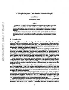
meas(p) = lub({meas(q) + 1 | p −→ q for some a}), where we assume lub(∅) = 0. If the ats is also finitely branching then all its states have finite measure. The notions of simulation and bisimulation provide important judgments on pairs of states in an abstract transition system. A good overview of relations on transitions systems (including simulation and bisimulation) can be found in [33]. A relation R ⊆ S × S is a simulation between p a a and q if and only if for every transition p −→ p0 , there exists a transition q −→ q 0 , such that p0 Rq 0 . The union of all simulations in an ats is also a simulation in the ats and we denote it by v; that is, p v q (read “q simulates p”) holds if and only if there exists a simulation R such that pRq. If p v q and q v p both hold, then p and q are similar. a A relation R is a bisimulation between p and q if and only if for every transition p −→ p0 , a a there exists a transition q −→ q 0 such that p0 Rq 0 , and for every transition q −→ q 0 , there exists a a transition p −→ p0 such that q 0 Rp0 . The union of all bisimulations in an ats is also a bisimulation in the ats and we denote it by ≡; that is, p ≡ q (read “p is bisimilar to q”) holds if and only if there exists a bisimulation R such that pRq. It is well-known that bisimilarity implies similarity but not vice-versa: for a counterexample, see Example 9. To illustrate our results, we will consider throughout the paper a more concrete example of an abstract transition system: the operational semantics of the concurrent language CCS [26]. For convenience, we ignore the renaming and hiding combinators, and concentrate on the sublanguage described by the grammar p ::= 0 | x | a.p | p + p | p | p | µx p, where x ranges over process variables and a ranges over a non-empty set of actions A, the set of ¯ the complementary actions A¯ = {¯ a | a ∈ A}, and {τ }, where τ ∈ / A ∪ A. The intended meaning of these symbols is as follows: 0 represents the inactive process, a.p represents a process prefixed by the action a, + and | are choice and parallel composition, respectively, and µx is the least fixed point operator, providing recursion. The operational semantics of CCS is specified by the transition rules in Figure 1. CCS can be seen as an abstract transition system where Λ = A ∪ A¯ ∪ {τ }, S is the set of all CCS expressions, and δ is the set of transitions which are derivable by the rules above. A finite CCS process is a CCS expression that does not contain µ. If S is restricted to the set of all finite CCS processes, then the resulting ats is noetherian. 6
B −→ B
initial
∆, B, C −→ E ⊗L ∆, B ⊗ C −→ E
∆ −→ B 1L ∆, 1 −→ B
−→ 1
1R
∆1 −→ B ∆2 −→ C ⊗R ∆1 , ∆2 −→ B ⊗ C
∆, B[y/x] −→ E ∃L ∆, ∃xB −→ E
∆ −→ B[t/x] ∃R ∆ −→ ∃xB
∆1 , C −→ E ∆2 −→ B −◦ L ∆1 , ∆2 , B −◦ C −→ E
∆, B −→ C −◦ R ∆ −→ B −◦ C
Figure 2: A proof system for a fragment of linear logic. The rule ∃L has the proviso that y is not free in the lower sequent.
4
Linear logic specification of abstract transition systems
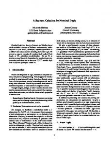
In this section, we will consider encoding abstract transition systems using linear logic and definitions. We will, in fact, use only the connectives 1, ⊗, −◦, and ∃, whose inference rules are given in Figure 2, along with def L and def R from Section 2. Before presenting our encoding, we state some properties of this combination of linear logic and definitions. The cut rule ∆1 −→ B B, ∆2 −→ C ∆1 , ∆2 −→ C is known to be admissible for this fragment of linear logic with definitions. This cut-elimination result is given by Girard in [12] or from the main result in [31]. In general, we shall only consider cut-free proofs when considering encodings of ats’s. Generally, there are many proofs for the same sequent, and many of these differ only in the order in which inference rules are applied. In particular, many inference rules permute over each other: if the order in which they are applied is switched, the proof would still be achieved in essentially the same way. Consider, for example, a proof that ends with the following two inference rules. ∆1 , C −→ D ∆2 −→ B −◦L ∆1 , ∆2 , B −◦ C −→ D ∆3 −→ E ⊗R. ∆1 , ∆2 , ∆3 , B −◦ C −→ D ⊗ E These instances of the −◦L and ⊗R can be permuted to yield ∆1 , C −→ D ∆3 −→ E ⊗R ∆1 , ∆3 , C −→ D ⊗ E ∆2 −→ B −◦L. ∆1 , ∆2 , ∆3 , B −◦ C −→ D ⊗ E In the case where the formula B −◦ C appears in the right premise of the ⊗R inference rule, a corresponding permutation is also possible. There are various pairs of inference rules that do not permute over each other. In the following Lemma, we write R1 /R2 to mean an occurrence of the inference rule R1 over the inference rule R2 . We do not need to consider permutations of two right-introduction rules since sequents have only one formula on their righthand-side. Lemma 5 The following pairs of inference rules do not permute over each other. 1R/1L
⊗R/⊗L
−◦ L/ −◦ R 7
−◦ L/⊗L
∃R/∃L
−◦L/def L
⊗R/def L
∃R/def L
def R/def L
All other pairs of inference rules permute. Proof We do not examine explicitly here all pairings of inference rules. Instead we show only a few cases: most cases are similar and simple. The case of nonpermutability of ⊗R/⊗L can be illustrated with the sequent p ⊗ q −→ q ⊗ p: this has a proof with an occurrence of ⊗L below ⊗R but there is no proof with ⊗R at the bottom. The other cases of nonpermutability can be shown by presenting similar counterexamples. Above, it has already been shown that the pair −◦L/⊗R permutes. Most of the other cases of permutability can be reasoned about as simply. The only difficult case involves showing that two atomic formulas on the left of a sequent can be introduced by the def L rule in either order: fortunately, this has already been proved in Section 2 (Proposition 4). The cases for def L/⊗R and def L/⊗L require applying substitutions to proofs, a notion formally defined in [20, 22]. To encode an ats in linear logic, we represent states as propositional constants. Actions will be represented by functional constants of type γ → γ, where γ is a new type. The sequence of actions, or trace, w = a1 · · · am (m ≥ 0) from Λ∗ will be encoded as the term w ˜ = λw.a1 (. . . (am w) . . .). (Here, the symbol denoting an action is also used to denote the corresponding function symbol.) Function composition represents the concatenation of traces: w1 w2 is encoded as w˜1 ◦ w˜2 = λw.w˜1 (w˜2 w). Besides the propositions that encode states, we need one other predicate tr of type (γ → γ) → o. Let ats 1 (δ) be the definition given by the following set of clauses: 4
ats 1 (δ) = {p = ∃W (tr(a ◦ W ) ⊗ (tr(W ) −◦ q)) | (p, a, q) ∈ δ}. Notice that the symbol denoting a state is also used to denote the corresponding logical atom. The following proposition shows how paths can be represented logically. w
Proposition 6 Let (Λ, S, δ) be an ats. Then p =⇒ q if and only if ats 1 (δ) ` ∀k((tr(k) −◦ q) −◦ (tr(w ˜ ◦ k) −◦ p)). Proof First notice that ats 1 (δ) ` ∀k((tr(k) −◦ q) −◦ (tr(w ˜ ◦ k) −◦ p)) if and only if ats 1 (δ) ` tr(w ˜ ◦ k), tr(k) −◦ q −→ p for any constant k of type γ → γ. We prove the reverse direction by induction on the length of w. Assume w is ² and that ats 1 (δ) ` tr(k), tr(k) −◦ q −→ p. The proof of this sequent cannot end with def L, since the predicate tr is not assumed to be defined. The proof cannot end with def R, since that would require the proof of tr(k) −→ tr(a ◦ w0 ) for some w0 , which is not provable. So the sequent can only ² be proved if it is the conclusion of an −◦L; thus, p and q are equal and p =⇒ q holds immediately. If w is not empty then it is of the form au. The proof of the sequent tr(a ◦ u ˜ ◦ k), tr(k) −◦ q −→ p cannot end with def L, since tr(a ◦ u ˜ ◦ k) is not a defined atom. It cannot end with −◦L, since that would require a proof of either −→ tr(k) or tr(a ◦ u ˜ ◦ k) −→ tr(k), neither of which are provable. a So the sequent must be the consequence of def R, there must be an r such that p −→ r, and the proof must be structured as follows: tr(˜ u ◦ k), tr(k) −◦ q −→ r tr(a ◦ u ˜ ◦ k) −→ tr(a ◦ u ˜ ◦ k) tr(k) −◦ q −→ tr(˜ u ◦ k) −◦ r tr(a ◦ u ˜ ◦ k), tr(k) −◦ q −→ tr(a ◦ u ˜ ◦ k) ⊗ (tr(˜ u ◦ k) −◦ r) tr(a ◦ u ˜ ◦ k), tr(k) −◦ q −→ ∃W (tr(a ◦ W ) ⊗ (tr(W ) −◦ r)) tr(a ◦ u ˜ ◦ k), tr(k) −◦ q −→ p 8
−◦R ⊗R ∃R def R.
This proof contains a subproof of tr(˜ u ◦ k), tr(k) −◦ q −→ r. By the inductive hypothesis, we have u au r =⇒ q and thus p =⇒ q. The proof in the forward direction is also by induction of the length of w. If w is empty, w then p =⇒ q implies that p and q are equal, and thus the sequent tr(w ˜ ◦ k), tr(k) −◦ q −→ p is provable (via −◦L and two uses of the initial rule). If w is nonempty then it is of the form a u au and there is some r such that p −→ r =⇒ q. By the inductive hypothesis, there is a proof of tr(˜ u ◦ k), tr(k) −◦ q −→ r. If we add to that proof the inference rules displayed above, we then get a proof of tr(a ◦ u ˜ ◦ k), tr(k) −◦ q −→ p. We prove now that with this encoding (along with def L), simulation corresponds to reverse linear implication. To do so, we introduce two new items. First, given a fixed ats (Λ, S, δ) and (p, q) ∈ S × S, a premise set for (p, q) is a set P ⊆ S × S such that for every a ∈ Λ and p0 ∈ S such a a that p −→ p0 there exists a q 0 ∈ S such that q −→ q 0 and (p0 , q 0 ) ∈ P . Premise sets need not exist, but if there is a simulation R that contains (p, q) then there is a premise set P for that pair such that P ⊆ R. We restrict premise sets to be minimal (assuming the axiom of choice). Notice also that premise sets can be empty. Second, we introduce the following class of inference rules: {p0 −→ q 0 | (p0 , q 0 ) ∈ P } SIM1 p −→ q where P is a premise set for (p, q). Notice that this rule is finitary if the ats is finitely branching. Let `SIM1 ∆ −→ C denote the proposition that the sequent ∆ −→ C can be proved using only the SIM1 inference rule. Lemma 7 Let (Λ, S, δ) be a noetherian ats and let p, q ∈ S. Then ats 1 (δ) ` p −→ q if and only if `SIM1 p −→ q. Proof Assume ats 1 (δ) ` p −→ q. If the proof of this sequent uses only the initial rule, then p and q are the same state. In a noetherian ats, a proof of p −→ p using only the SIM1 inference rule can always be constructed, a result that follows from a simple induction on meas(p). (This is the only use of the noetherian assumption in this proof.) Otherwise, the only inference rules that can be applied to prove such a sequent are either def R or def L since p and q are atomic formulas. By Lemma 5, occurrences of def L can be permuted down over def R and the right introduction rules for ∃, ⊗, and −◦. So we can assume that the last inference rule used to prove this sequent is def L, and thus the proof has the form a
{∃W (tr(a ◦ W ) ⊗ (tr(W ) −◦ p0 )) −→ q | p −→ p0 } def L. p −→ q Consider one of these premises, say, ∃W (tr(a ◦ W ) ⊗ (tr(W ) −◦ p0 )) −→ q. Given the permutations of the inference rules listed in Lemma 5, we can assume that this premise is obtained by left introduction rules for ∃ and ⊗, yielding the sequent tr(a ◦ w), tr(w) −◦ p0 −→ q where w is a variable. The proof of this sequent cannot end with def L since tr(a ◦ w) is not a defined atom. It also cannot end with −◦L since this would require a proof of either −→ tr(w) or tr(a ◦ w) −→ tr(w), neither of which are provable. Therefore, the proof must end with def R, which yields the sequent tr(a ◦ w), tr(w) −◦ p0 −→ ∃W (tr(b ◦ W ) ⊗ (tr(W ) −◦ q 0 )), b
where q −→ q 0 . There is a proof of this sequent, however, only if a = b and ∃W is instantiated with w (using the ∃ right introduction rule), bringing us to the sequent tr(a ◦ w), tr(w) −◦ p0 −→ tr(a ◦ w) ⊗ (tr(w) −◦ q 0 ). 9
A proof of this sequent must end with the right introduction rules for ⊗ and −◦ and the left introduction rule for −◦, and contain a subproof of the sequent p0 −→ q 0 . Thus, if we collect all such pairs (p0 , q 0 ) into the set P , we have a premise set for (p, q) and we have established an instance of the SIM1 rule. Since all these proof steps are forced, this proves the completeness of SIM1 . The converse follows simply by noting that each instance of the SIM1 inference rule can be built using several instances of inference rules from linear logic, one instance of def L, and possibly several instances of def R. Notice that for a noetherian ats we do not need instances of the initial sequent rule to be used with defined atoms: a proof of p −→ p can be obtained using only the SIM1 rule or the corresponding combination of def L, def R, ∃L, ∃R, ⊗L, ⊗R, −◦L, −◦R, and the initial rule for undefined atoms. This observation is similar to the one that holds of most proof systems: the initial rule is needed to prove A −→ A only when A is atomic; that is, when A has a non-logical symbol as its head symbol. When using ats 1 (δ) as a definition, states become logical constants (in the sense that they have left and right introduction rules), and hence we do not need any instance of the initial rule. Notice, however, if we did admit the initial inference rule along with the SIM1 inference rule, the previous lemma could be extended to the non-noetherian case. We can now establish our first proof theoretic connection to simulation. Theorem 8 Let (Λ, S, δ) be a noetherian ats and let p, q ∈ S. Then ats 1 (δ) ` p −→ q if and only if q simulates p. Proof Given Lemma 7, we need only show that `SIM1 p −→ q if and only if q simulates p. First, assume that the sequent p −→ q has a proof that contains only instances of the SIM1 inference rule. Let R be the set of all pairs (r, s) such that the sequent r −→ s has an occurrence in that proof. It is easy to verify that R is a simulation. Conversely, assume that q simulates p. Thus there is a simulation R such that pRq. The proof is by complete induction on the measure of p, meas(p). Since pRq, there is a premise set P ⊆ R for (p, q). If (p0 , q 0 ) ∈ P , then p0 Rq 0 and meas(p0 ) < meas(p), so we have by the induction hypothesis `SIM1 p0 −→ q 0 . Thus, we have proved `SIM1 p −→ q. This theorem states that in a noetherian ats, simulation can be identified with the logical connective −◦ via the encoding ats 1 (δ). As a consequence, logical equivalence of p and q, namely the provability of both p −◦ q and q −◦ p, corresponds to similarity of p and q, i.e. simulation in both directions. Notice that bisimilarity implies similarity but does not coincide with it, as the following example shows. Hence logical equivalence is coarser than bisimulation equivalence. Example 9 Consider the transition system with one label a, states {p1 , p2 , p3 , p4 , q1 , q2 , q3 }, and a a a a a transitions p1 −→ p2 , p2 −→ p3 , p1 −→ p4 , q1 −→ q2 , q2 −→ q3 . The relations {(p1 , q1 ), (p2 , q2 ), (p3 , q3 ), (p4 , q2 )} and {(q1 , p1 ), (q2 , p2 ), (q3 , p3 )} witness the fact that q1 simulates p1 and p1 simulates q1 , respectively. It is easy to check, however, that there is no bisimulation that contains the pair (p1 , q1 ). As a consequence of this example, we see no way to make bisimilarity into a logical connective; that is, into a constant of type o → o → o with left and right introduction rules that enjoys cut-elimination. In the special case of noetherian and determinate ats, however, similarity implies bisimilarity, and hence logical equivalence and bisimulation equivalence coincide.
10
∆, B −→ B
initial
∆, B, C −→ E ∧L ∆, B ∧ C −→ E
∆ −→ >
>R
∆ −→ B ∆ −→ C ∧R ∆ −→ B ∧ C
∆, B[t/x] −→ C ∀L ∆, ∀xB −→ C
∆ −→ B[y/x] ∀R ∆ −→ ∀xB
∆, B[y/x] −→ E ∃L ∆, ∃xB −→ E
∆ −→ B[t/x] ∃R ∆ −→ ∃xB
∆, C −→ E ∆ −→ B ⊃L ∆, B ⊃ C −→ E
∆, B −→ C ⊃R ∆ −→ B ⊃ C
Figure 3: A proof system for a fragment of intuitionistic logic. The rules ∀R and ∃L have the proviso that y is not free in the lower sequent of that inference rule. The structural rules of exchange and contraction are implicit in the use of sets on the left-hand side of the sequent arrow. The weakening rule is implicit in the presence of ∆ in the axioms. Proposition 10 Let (Λ, S, δ) be a noetherian and determinate ats and let p, q ∈ S. Then ats 1 (δ) ` p −◦ q and ats 1 (δ) ` q −◦ p if and only if p is bisimilar to q. Proof We prove that if the ats is noetherian and determinate then similarity and bisimilarity coincide. The proposition then follows from Theorem 8. We show that similarity implies bisimulaa rity by well-founded induction on meas(p). Consider a transition p −→ p0 . Since p v q, there must a exist a q 0 such that q −→ q 0 and p0 v q 0 . Since the ats is determinate, q v p implies q 0 v p0 . Since a meas(p0 ) < meas(p), the inductive hypothesis yields p0 ≡ q 0 . Symmetrically, for any q −→ q 0 , there a exist p −→ p0 such that q 0 ≡ p0 . Therefore p ≡ q.
5
Encoding one-step transitions as atomic judgments
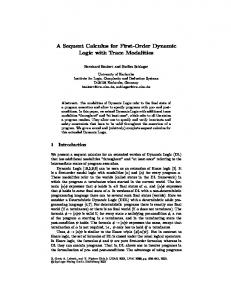
While using linear logic directly to encode transitions was rather natural and immediate, the resulting encoding will not be able to provide us information about bisimilarity in many situations, as is illustrated in Example 9. To overcome this problem we give a second encoding of abstract transition systems, this time encoding the relations between states as predicates rather than logical connectives. Since this encoding will not need linearity, it uses intuitionistic logic instead. Definitions will play a role rather similar to the one they played in the previous encoding. Consider intuitionistic logic using the connectives > for true, ∧ for conjunction, ⊃ for implication, and ∀ and ∃ for universal and existential quantification. Sequents for this intuitionistic logic are of the form ∆ −→ B where ∆ is a set of formulas and B is a formula. The sequent calculus for this fragment of intuitionistic logic is given in Figure 3. Schroeder-Heister showed in [31] that if definitions do not contain implications in clause bodies, then cut-elimination can be proved for intuitionistic logic extended with def L and def R rules. However, we shall need a strong form of definition that allows certain stratified occurrences of implications. In particular, we assume that each predicate symbol p in the language has associated with it a natural number lvl(p), the level of the predicate. The notion of level is then extended to formulas as follows. Given a formula B, its level lvl(B) is defined as follows: lvl(p(t¯)) = lvl(p), lvl(>) = 0, lvl(B ∧ C) = max(lvl(B), lvl(C)), lvl(B ⊃ C) = max(lvl(B) + 1, lvl(C)), and lvl(∀x.B) = lvl(∃x.B) = lvl(B). We say that a defini11
4
∀P [ multi(P, nil, P ) = >] 4 ∀A, P, Q, W [ multi(P, A :: W, Q) = ∃R(one(P, A, R) ∧ multi(R, W, Q))] Figure 4: The definition path. 4
tion is stratified if for every clause ∀¯ x[H = B] of that definition, lvl(B) ≤ lvl(H). It is proved in [22] that cut can be eliminated from intuitionistic logic extended with stratified definitions. In the rest of this paper, when we use the term “definition” we shall mean “stratified definition”. The following Lemma is similar to Lemma 5 and is proved similarly. Lemma 11 The following pairs of inference rules do not permute over each other. We write R1 /R2 to mean an occurrence of inference rule R1 over inference rule R2 . ∀L/∀R
⊃L/⊃R
∃R/∃L
∀L/∃L
∃R/def L
∀L/def L
def R/def L
All other pairs of inference rules permute. Let (Λ, S, δ) be an ats and let the primitive types σ and α denote the type of the elements in S and Λ, respectively. Let one: σ → α → σ → o be a predicate denoting the one-step transition relation δ. Let ats 2 (δ) be the definition given by the following set of clauses: 4
ats 2 (δ) = {one(p, a, q) = > | (p, a, q) ∈ δ}. To encode paths within a transition system we use the predicate multi : σ → list(α) → σ → o, which is defined by the definition path given in Figure 4. The predicates one and multi are assumed to have level 0. Here, members of Λ∗ are represented as terms of type list(α) using nil : list(α) for the empty list and :: of type α → list(α) → list(α) for the list constructor. The following proposition should be contrasted to Proposition 6; its proof is simpler. w
Proposition 12 Let (Λ, S, δ) be an ats. Then ats 2 (δ), path ` multi(p, w, q) if and only if p =⇒ q. The encoding ats 2 (δ) is based on an extensional description of δ, hence the definition will be infinite if δ is infinite. In specific transition systems the transition relation might be described structurally. This is the case for CCS, whose transitions can be encoded as the definition ccs(A), given in Figure 5. Here the combinators of CCS are typed as follow: the action prefix has type α → σ → σ, the + and | both have type σ → σ → σ, and µ has type (σ → σ) → σ. We assume the silent action τ : α is not a member of the set A. Observe that we are using meta-level λ-abstraction to encode µx P : such a term is represented as µM , where M is meant to be the abstraction λx.P . Thus the term P [µx P/x] can be represented simply by M (µM ) without introducing an explicit notion of substitution (β-conversion in the meta-logic performs the necessary substitution). The following result shows that CCS transitions are completely described by logical derivability in ccs(A). a
w
Proposition 13 The transition p −→ q holds if and only if ccs(A) ` one(p, a, q), and p =⇒ q holds if and only if ccs(A), path ` multi(p, w, q).
12
∀A, P [ one(A.P, A, P ) ∀A, P, Q, R [ one(P | R, A, Q | R) ∀A, P, Q, R [ one(R | P, A, R | Q) ∀A, P, Q, R [ one(P + R, A, Q) ∀A, P, Q, R [ one(P + R, A, Q) ∀A, P, Q [ one(µM, A, Q) ∀P, Q, R, S [ one(P | Q, τ, R | S)
4
= 4 = 4 = 4 = 4 = 4 = 4 =
>] one(P, A, Q)] one(P, A, Q)] one(P, A, Q)] one(R, A, Q)] one(M (µM ), A, Q)] ∃A, B(comp(A, B) ∧ one(P, A, R) ∧ one(Q, B, S))] 4
4
For each a ∈ A, the two clauses comp(a, a ¯) = > and comp(¯ a, a) = >. Figure 5: The definition ccs(A). Here, A is a non-empty set of actions. 4
= ∀A∀P 0 . one(P, A, P 0 ) ⊃ ∃Q0 . one(Q, A, Q0 ) ∧ sim(P 0 , Q0 )] 4 ∀P, Q [ bisim(P, Q) = [∀A∀P 0 . one(P, A, P 0 ) ⊃ ∃Q0 . one(Q, A, Q0 ) ∧ bisim(P 0 , Q0 )] ∧ [∀A∀Q0 . one(Q, A, Q0 ) ⊃ ∃P 0 . one(P, A, P 0 ) ∧ bisim(Q0 , P 0 )]]
∀P, Q [
sim(P, Q)
Figure 6: The definition sims. This proposition can be proved by simple structural induction by showing that proofs using the inference rules in Figure 1 for CCS are essentially identical to sequent calculus proofs over the corresponding clauses in the definition ccs(A). Notice that the sequent calculus proofs involve only right introduction rules. If we explicitly represent the transition step by a predicate one (defined by ats 2 (δ) or by a system like ccs(A)), then it is possible to characterize simulation and bisimulation as predicates sim and bisim given by the definition sims, presented in Figure 6. Since the level of one is 0, we need to assign to both sim and bisim the level 1 (or higher) in order to make this definition stratified. In order to prove that these encodings correctly capture simulation and bisimulation, we need to show that we can restrict the use of the def L rule without affecting provability. Toward that end we introduce another version of the left introduction rule for definitions, def Lnc . This version is the same as def L but with the additional restriction that the introduced atom is not a member of the side formulas on the left: 4
{Bθ, ∆θ −→ Cθ | θ ∈ csu(A, H) for some clause ∀¯ x.[H = B]} def Lnc , provided A ∈ / ∆. A, ∆ −→ C As before, the variables x ¯ in this rule need to be chosen so that they are not free in any formula of the lower sequent. We shall show that in a proof of the sequents −→ sim(p, q) or −→ bisim(p, q), this additional restriction does not affect provability. We shall call an instance of def L redundant if it is not an instance of def Lnc . A proof in which all instances of def L are instances of def Lnc is a proof without redundancies. Proposition 14 Let (Λ, S, δ) be an ats and let p, q ∈ S. 13
• If ats 2 (δ), sims ` sim(p, q), then there is also a proof of −→ sim(p, q) without redundancies, and • If ats 2 (δ), sims ` bisim(p, q), then there is also a proof of −→ bisim(p, q) without redundancies. The same holds if we replace ats 2 (δ) by ccs(A) and restrict p and q to be finite processes. Proof We shall show how to replace a redundant instance of def L at the root of a proof by an instance of def Lnc . By repeatedly removing such redundant instances, we can convert a proof using def L into a proof using def Lnc . Consider a proof of A, ∆ −→ C in which that sequent is the consequence of a redundant application of def L that introduces A. Thus, ∆ = {A} ∪ ∆0 for some ∆0 that does not contain A. Also assume that this proof contains no other redundant occurrences of def L. We shall transform this proof into one of A, ∆0 −→ C that uses only def Lnc . The premise of this occurrence of def L is the set of sequents 4
{Bθ, ∆θ −→ Cθ | θ ∈ csu(A, H) for some clause ∀¯ x[H = B]}. For each of the sequents Bθ, Aθ, ∆0 θ −→ Cθ we construct a proof of Bθ, ∆0 θ −→ Cθ as follows. 4 Since there is a definitional clause ∀¯ x[H = B] such that Aθ = Hθ, there is a proof of the sequent Bθ −→ Aθ using def R and initial. Using the cut-elimination theorem of [22], we know there is a (cut-free) proof of Bθ, ∆0 θ −→ Cθ. (Since the left-hand side of the sequent is a set, we can combine the two occurrences of Bθ.) We can use all of these proofs of the sequents Bθ, ∆0 θ −→ Cθ and an instance of the def L rule to prove the sequent A, ∆0 −→ C. To guarantee that this new proof does not contain redundant occurrences of the def L rule, we need to know that the cut-elimination process does not introduce new redundant occurrences, and also that the implicit contraction on Bθ in the premises does not result in a new redundant occurrence. The cut-elimination procedure in [22] can only introduce redundant occurrences of the def L rule if there are occurrences of ⊃L or natL in the proof. An examination of the relevant formulas and definitions reveals that the only formulas that will be on the left-hand side of a sequent in a cut-free proof of −→ sim(p, q) or −→ bisim(p, q) will be atomic formulas constructed using the predicate one (and the predicate comp in the CCS case). Thus the proof will not contain occurrences of the ⊃L or natL rules, so cut-elimination will not introduce redundant occurrences of def L. The implicit contraction of Bθ will introduce a redundant occurrence of def L only if Bθ is the main formula of an occurrence of def L. Remember that B is the body of a definitional clause 4 ∀¯ x[H = B] such that θ ∈ csu(A, H), and A is an atomic formula constructed using either one or comp. With the definition ats 2 (δ), B will always be the formula >, which cannot be the main formula of def L. With the definition ccs(A), however, B may be another atomic formula constructed using one, and so may be the main formula of def L. Since we have excluded the µ operator, the first argument to one in B is necessarily a subexpression of the first argument to one in A. This provides us with a measure that guarantees that any new redundant occurrence of def L that is introduced is strictly smaller than the one eliminated. Since our definition is finite, the original occurrence of def L will have a finite number of premises, so at most a finite number of new redundant occurrences are introduced. As a result, we can apply the elimination process to the new occurrences, and eventually the process will terminate.
14
We now introduce an inference rule similar to the SIM1 rule given above, namely {−→ sim(p0 , q 0 ) | (p0 , q 0 ) ∈ P } SIM2 −→ sim(p, q) where P is a premise set for (p, q). We also present an inference rule for bisimulation: {−→ bisim(p0 , q 0 ) | (p0 , q 0 ) ∈ P } ∪ {−→ bisim(q 0 , p0 ) | (q 0 , p0 ) ∈ Q} BISIM2 −→ bisim(p, q) where P is a premise set for (p, q) and Q is a premise set for (q, p). Again, these rules are finitary if the ats is finitely branching. In the case of CCS, one condition which guarantees this property is that recursion variables in bodies of µ-terms only occur prefixed. Let `SIM2 ∆ −→ C (respectively, `BISIM2 ∆ −→ C) denote the proposition that the sequent ∆ −→ C can be proved using only occurrences of the SIM2 (respectively, BISIM2 ) inference rule. The following lemma is the analogue of Lemma 7 for this second encoding. Lemma 15 Let (Λ, S, δ) be an ats and let p, q ∈ S. Then • ats 2 (δ), sims ` sim(p, q) if and only if `SIM2 sim(p, q), and • ats 2 (δ), sims ` bisim(p, q) if and only if `BISIM2 bisim(p, q). The same holds if we replace ats 2 (δ) by ccs(A) and restrict p and q to be finite processes. Proof We outline the proof of the first case; the second can be done similarly. Consider a proof of the sequent −→ sim(p, q). This is provable only by a def R rule using sims, and thus the sequent −→ ∀A∀P 0 . one(p, A, P 0 ) ⊃ ∃Q0 . one(q, A, Q0 ) ∧ sim(P 0 , Q0 ) must be provable. The only (cut-free) proof of this sequent must end in three occurrences of right-introduction rules and a proof of the sequent one(p, A, P 0 ) −→ ∃Q0 . one(q, A, Q0 ) ∧ sim(P 0 , Q0 ) (here, A and P 0 are variables introduced by the ∀R rule). By permuting inference rules, we can assume that this latter sequent is proved with def L (or more precisely def Lnc ) and that its premises, namely the sequents −→ ∃Q0 . one(q, a, Q0 ) ∧ sim(p0 , Q0 ), where the pair (a, p0 ) ranges over hhpii, are each provable. Such a sequent is provable only if the a quantifier ∃Q0 is instantiated with q 0 where q −→ q 0 . Let P be the premise set arising from collecting together all pairs (p0 , q 0 ) for such values p0 and q 0 . Thus, our original sequent is provable if and only if for every (p0 , q 0 ) ∈ P the sequent −→ sim(p0 , q 0 ) is provable. The other direction follows by reversing these reasoning steps. Now the following can be proved using Lemma 15 in a manner analogous to the proof of Theorem 8 using Lemma 7. Theorem 16 Let (Λ, S, δ) be a noetherian ats, and let p and q be members of S. Then • ats 2 (δ), sims ` sim(p, q) if and only if p v q, and 15
• ats 2 (δ), sims ` bisim(p, q) if and only if p ≡ q. Concerning CCS, the full language is not noetherian because of the presence of the recursion operator. If we consider only expressions without µ, i.e. finite processes, then the same property holds, as is witnessed by the following theorem. We omit the proof of this theorem since it is essentially the same as the preceding proof: the main difference is that the definition of the onestep transitions for CCS is a recursive definition. Theorem 17 The following equivalences hold for finite processes p and q of CCS. • ccs(A), sims ` sim(p, q) if and only if p v q. • ccs(A), sims ` bisim(p, q) if and only if p ≡ q.
6
Infinite behavior
As we mentioned in Section 2, a definition can be seen as defining the predicates in the heads of the clauses by mutual recursion. Notice that we use the technique of stratification to give meaning to definitions containing implications. For a discussion on stratified specifications in the presence of negation (which can be reduced to a use of implication), see, for example, [1]. We now examine how such recursive definitions can be viewed as fixed points of suitable operators. The clauses for defining the level 0 predicate one (both for ats 2 (δ) and for ccs(A)) are Horn 4 clauses when = is replaced with reverse implication. The usual meaning of predicates defined by Horn clauses is given by the least fixed point of the monotone, one-step inference operator associated with the clauses [2]. In our case, this interpretation for the predicate one coincides with the transition relation. That is, one(p, a, p0 ) is a member of the least fixed point if and only if a p −→ p0 . For the definition ats 2 (δ), this is trivial, and for the definition ccs(A), this follows from Proposition 13 and the fact that the least fixed point characterizes the set of atomic consequences [2]. We now define an analogous one-step inference operator associated with the definition sims. In that definition, simulation and bisimulation are predicates of level 1 and the clauses are of the 4 form ∀P ∀Q[r (P, Q) = Φ], where the formula Φ contains free occurrences of the variables P and Q, strictly positive occurrences of the predicate r (namely, sim or bisim), and both positive and negative occurrences of the predicate one. With such a clause we associate a function φ from binary relations to binary relations whose definition corresponds to the formula Φ, except that a atomic formulas of the form one(p, a, p0 ) are replaced with their denotation, namely, p −→ p0 . We are following here the classical approach to the fixed point semantics of stratified definitions: first, we determine the meaning of predicates of level lower than n; then their meaning is used in the definition of the one-step inference operator for predicates of level n. Since in the definition of the latter the predicate occurring negatively must have level lower than n, this techniques ensures that the one-step inference operator is monotone and thus has fixed points. In general, there will be more than one such fixed point. Notice that both def L and def R are sound for all the relations which are fixed points of φ. To see this, assume that for any relation r there is only one such definitional clause (in case there are more, we group them in one clause which has as body the disjunction of the bodies). Then 4 observe that the use of def L corresponds to replacing = by ⊃ in the clause, that is, to assuming the formula ∀P ∀Q[r (P, Q) ⊃ Φ]. The case for def R corresponds to the converse: that is, to replacing 4 = with ⊂.
16
Let Φs and Φb be the bodies of the clauses given in sims for sim and bisim, respectively, and consider the following corresponding functions φs and φb , on binary relations, associated with these formulas. A
A
φs (R) := {(P, Q) | ∀A ∈ Λ∀P 0 ∈ S if P −→ P 0 then ∃Q0 such that Q −→ Q0 and (P 0 , Q0 ) ∈ R} A A φb (R) := {(P, Q) | [∀A ∈ Λ∀P 0 ∈ S if P −→ P 0 then ∃Q0 such that Q −→ Q0 and A (P 0 , Q0 ) ∈ R] and [∀A ∈ Λ∀Q0 ∈ S if Q −→ Q0 then ∃P 0 such A that P −→ P 0 and (Q0 , P 0 ) ∈ R]} We can see from their definitions that v and ≡ are the greatest fixed points of φs and φb , respectively. Notice that in proofs of −→ sim(p, q) and −→ bisim(p, q) using definitions ats 2 (δ) and sims, def L is used with ats 2 (δ) but not with sims. As the following example shows, when the transition system is not noetherian, the “if” parts of Theorem 16 may not hold. Example 18 Consider a transition system with two states only, p and q, and two transitions a a p −→ p and q −→ q. Then p v q holds, but sim(p, q) cannot be proved. Notice that an attempt to prove it would end up in a circularity. Notice that ats 2 (δ), sims ` sim(p, q) holds if and only if (p, q) is contained in every fixed point of φs and that ats 2 (δ), sims ` bisim(p, q) holds if and only if (p, q) is contained in every fixed point of φb . In a noetherian ats, φs and φb have unique fixed points, and it is for this reason that v and ≡ can be completely characterized in a noetherian ats by provability (Theorem 16). One attempt to characterize the greatest fixed point of the relation transformer φ prooftheoretically is to introduce a notion of “proof with finite or infinite height”. An ω-proof of the sequent ∆ −→ C with inference rules taken from the set L is a tree whose root is labeled by ∆ −→ C, and such that for every node N there is an instance of an inference rule of L whose conclusion is the label of N , and whose premises are the labels of the children of N . We will denote by `ωL ∆ −→ C the existence of an ω-proof in L for ∆ −→ C. For example, `ωSIM2 ∆ −→ C is true if ∆ −→ C has an ω-proof using only SIM2 . If the set L of inference rules is determined by those in intuitionistic logic and instances of def Lnc and def R for some definition D, then we write D `ω ∆ −→ C. Notice that an ω-proof can have finite or infinite height, and that this is orthogonal to the proof being finitely or infinitely branching, which is related to the possibility of having infinitary rules. We prove now that Lemma 15 still holds for ω-proofs. Lemma 19 Let (Λ, S, δ) be an ats and let p, q ∈ S. Then • ats 2 (δ), sims `ω sim(p, q) if and only if `ωSIM2 sim(p, q), and • ats 2 (δ), sims `ω bisim(p, q) if and only if `ωBISIM2 bisim(p, q). Proof We outline the proof of the first case; the second can be done similarly. Since the converse is immediate, we only show the forward direction. Assume that the sequent −→ sim(p, q) has an ω-proof using the definition ats 2 (δ). Since this sequent must be proved by one use of def R, two uses of ∀R, and one use of ⊃R, we have ats 2 (δ) `ω one(p, A, P 0 ) −→ ∃q 0 [one(q, A, q 0 ) ∧ sim(P 0 , q 0 )], 17
where A and P 0 are variables. At this point, the proof can proceed by either def L or ∃R. If the choice is def L, then we quickly get that the proof is essentially an instance of SIM2 at the root, and we proceed recursively through the ω-proof. Otherwise, a use of ∃R would give rise to a conjunction, the first component of which is one(q, A, q0 ) for some particular q0 ∈ S. It is not possible, however, to prove this atom using def R since no instance of a clause in the definition ats 1 (δ) has the variable A in its head. Thus, this proof could not be built in that fashion. It is important for this Lemma that we use def Lnc (see Section 5) and not def L since the latter can lead to infinite sequences of redundant occurrences of def L. We can now extend Theorem 16 to ω-proofs and drop the noetherian condition. Theorem 20 Let (Λ, S, δ) be an ats, and let p and q be members of S. Then • ats 2 (δ), sims `ω sim(p, q) if and only if p v q, and • ats 2 (δ), sims `ω bisim(p, q) if and only if p ≡ q. Proof We prove only the first equivalence since the second follows similarly. First, assume that ats 2 (δ), sims `ω sim(p, q). By Lemma 19, `ωSIM2 sim(p, q). Let Ξ be a proof of −→ sim(p, q) that contains just the SIM2 inference rule and let R be the binary relation such that rRs if r −→ s has an occurrence in Ξ. It is easy to see that R is a simulation containing (p, q). Assume next that p v q holds. We construct a monotonic sequence of trees {Tk }k∈ω such that for every k, the root of Tk is labeled by −→ sim(p, q), all the leaves of Tk are labeled by sequents of the form −→ sim(p0 , q 0 ) where p0 v q 0 holds, and Tk+1 is obtained from Tk by attaching to each leaf of Tk an appropriate instance of SIM2 . T0 is the tree consisting solely of the node labeled −→ sim(p, q). Given Tk , for every leaf labeled −→ sim(p0 , q 0 ), we know that 0 ),. . . , where {(a , p0 ), . . . , (a , p0 ), . . .} = hhp0 ii p0 v q 0 , so v contains pairs (p01 , q10 ), . . . , (p0m , qm 1 1 m m 0 ), . . .} ⊆ hhqii for some actions a , . . . , a , . . .. Hence in T and {(a1 , q10 ), . . . , (am , qm 1 m k+1 the sequent p0 −→ q 0 can be placed at the conclusion of a SIM2 rule, whose premises are p01 −→ q10 , . . . , p0m −→ 0 , . . .. The limit of this sequence {T } qm k k∈ω is an ω-proof for sim(p, q) using occurrences of the SIM2 rule. The application of Lemma 19 yields the conclusion ats 2 (δ), sims `ω sim(p, q). For Lemma 19 and Theorem 20 to hold, it is important that the relation one be defined in a “noetherian” way itself. If we consider a recursive definition for one, like in ccs(A) (with the clause for µ), then the reverse direction of these equivalences does not necessarily hold, as the following example illustrates. Example 21 The CCS terms µx x and µx a.x are such that neither `ωSIM2 sim(µx a.x, µx x) nor µx a.x v µx x hold. However, the judgment ccs(A), sims `ω sim(µx a.x, µx x) holds. a
In fact, notice that µx x −→ µx a.x does not hold, while ccs(A) `ω one(µx x, a, µx a.x). The infinite proof of one(µx x, a, µx a.x) is in a sense an “infinite failure”. If we restrict to finite CCS processes, then such infinite failures do not occur with respect to the one step transition steps and the only infinite proof behaviors will be those that positively verify the greatest fixed point properties of simulation and bisimulation. Thus, when restricted to finite CCS processes, the variation of Theorem 20 where ats 2 (δ) is replaced with ccs(A) holds.
7
An inductive encoding of simulation and bisimulation
In previous sections we have shown how to encode in sequent calculus various relations over the states of a transition system. We now explore the kinds of properties on the relations that can 18
be proved within the calculus or via some characterization provided by the calculus. We will see that several properties cannot be proved within the logic because their proof requires inductive reasoning. We will then discuss one possible approach to enhance sequent calculus with induction. Example 22 The property “bisimulation is preserved by the prefix operator” holds in CCS. The corresponding encoding of this property is also provable in the sequent calculus; that is, we have ccs(A), sims ` ∀A∀P ∀Q[bisim(P, Q) ⊃ bisim(A.P, A.Q)], which is easy to verify. Example 23 The properties “bisimulation is symmetric” and “bisimulation is transitive” hold in any transition system. The corresponding encodings of these two properties are also provable in the sequent calculus; that is, we have ats 2 (δ), sims ` ∀P ∀Q[bisim(P, Q) ⊃ bisim(Q, P )] and ats 2 (δ), sims ` ∀P ∀Q∀R[bisim(P, Q) ∧ bisim(Q, R) ⊃ bisim(P, R)], both of which are easy to verify. As the following examples illustrate, there are plenty of properties of ≡ and v that cannot be proved within the logic. In fact, as we already observed, we can prove properties of sim and bisim only if they are true for every fixed point of φs and φb , but in the non-noetherian case there is in general more than one fixed point. Example 24 The property “bisimulation equivalence implies the largest simulation” (or more formally: ≡ is a subset of v) is true in any transition system. This property can be expressed by the formula ∀P ∀Q[bisim(P, Q) ⊃ sim(P, Q)] but, in general, if δ is a non-noetherian transition relation, this formula cannot be proved using the definitions ats 2 (δ) and sims. For example, if we take the transition system ({a}, {p}, {(p, a, p)}) it is immediate to see that {(p, p)} is a bisimulation (the greatest fixed point of φb , namely bisimulation equivalence) and ∅ is a simulation (the least fixed point of φs ). Hence, this formula cannot be proved for this transition system. Example 25 The property “bisimulation equivalence is reflexive” holds in any transition system. The formula ∀P [bisim(P, P )] cannot be proved using the definitions ats 2 (δ) and sims. Consider for instance the same transition system as in Example 24: the empty set ∅ is a bisimulation (the least fixed point of φb ), and it is, of course, not reflexive. Example 26 The property “bisimulation equivalence is preserved by the + operator” is true in CCS. This property can be expressed as the formula ∀P ∀Q∀R[bisim(P, Q) ⊃ bisim(P + R, Q + R))]. This sequent cannot be proved using ccs(A) and sims. In fact, take P = a.0, Q = a.0 + a.0 and R = µx a.x. The least fixed point of φb contains the pair (a.0, a.0 + a.0) but not the pair (a.0 + µx a.x, a.0 + a.0 + µx a.x). The notion of “infinite proof”, introduced in the previous section, can be helpful to prove properties on the defined relations at the meta (mathematical) level. For instance, the properties in Examples 24 and 25 can both be proved by using the characterization of ≡ and v provided at the end of the previous section. It is easy to see, in fact, that ccs(A), sims `ω bisim(P, P ). Concerning the 19
implication bisim(P, Q) ⊃ sim(P, Q), observe that any infinite proof for −→ bisim(P, Q) contains an infinite proof of −→ sim(P, Q). The characterization of simulation or bisimulation using ω-proofs is not so helpful because the existence of an infinite proof for a given sequent is co-semidecidable but (in general) not semidecidable. A better approach would be to use induction to capture the greatest fixed point. In particular, define the binary relations vi and ≡i for each natural number i as follows. Both T v0 and ≡0 are defined to be S × S, and vi+1 := φs (vi ) and ≡i+1 := φb (≡i ). Now set vω := i vi T and ≡ω := i ≡i . It is easy to show that for finitely-branching transition systems, φs and φb are downwardcontinuous and, hence, v equals vω and ≡ equals ≡ω . A simple induction shows that for i ≥ 0, v ⊆ vi and ≡ ⊆ ≡i and thus v ⊆ vω and ≡ ⊆ ≡ω . The converse needs the finitely branching assumption and follows from Theorem 5.6 of [25]. In CCS, finite branching is guaranteed whenever all the recursion variables in µ-expressions are prefixed. Thus, one approach to showing that two states are bisimilar is to show that for all natural numbers i, those two states are related by ≡i . Such statements can often be proved by induction on natural numbers. We can incorporate induction into our proof systems by introducing natural numbers using z for zero and s for successor and using the predicate nat and the following “introduction” rules for this new predicate. ∆ −→ nat(z)
natR
∆ −→ nat(x) natR ∆ −→ nat(s(x))
−→ Q(z) Q(y) −→ Q(s(y)) ∆, Q(x) −→ P natL nat(x), ∆ −→ P Here, x, P , and Q are schematic variables of these inference rule, and y is a variable not free in Q. The first two rules can be seen as right introduction rules for nat while the third rule, encoding induction over natural numbers, can be seen as a left introduction rule. In the left introduction rule, Q ranges over formulas with one variable extracted (say, using λ-abstraction) and represents the property that is proved by induction: the third premise of that inference rule witnesses the fact that, in general, Q will express a property stronger than P . The paper [22] contains a proof that cut-elimination holds for intuitionistic logic extended with both these rules for natural numbers and with stratified definitions. Notice that with this formulation of induction, cut-free proofs will not have the subformula property. We use `IN to denote provability using both left and right introduction rules for definitions as well as the above mentioned left and right rules for natural numbers. If n is a natural number, we write n ¯ to denote the corresponding “numeral” for n: that is, n ¯ is the term containing n occurrences of s and one occurrence of z. We can now encode vi and ≡i by using the indexed versions of sim and bisim given by the relations ssim and sbisim, respectively, defined in Figure 7. We will denote this definition as ssims. The following proposition shows how a proof using induction can yield proofs that do not involve induction. Proposition 27 Let (Λ, S, δ) be an ats, and let p and q be members of S. If ats 2 (δ), ssims `IN n, p, q). If ats 2 (δ), ssims `IN sim(p, q) then for every natural number n, ats 2 (δ), ssims ` ssim(¯ bisim(p, q) then for every natural number n, ats 2 (δ), ssims ` sbisim(¯ n, p, q). Proof We prove the first result about simulation: the result about bisimulation is analogous. A cut-free proof of the sequent −→ sim(p, q) must end in a def R rule, which (using ∀R and ⊃R also) means that the sequent nat(k) −→ ssim(k, p, q) is provable, where k is a variable. Call this 20
4
sim(P, Q) = ∀K. nat(K) ⊃ ssim(K, P, Q). 4 ssim(z, P, Q) = > 4 ssim(s(K), P, Q) = [∀A∀P 0 . one(P, A, P 0 ) ⊃ ∃Q0 . one(Q, A, Q0 ) ∧ ssim(K, P 0 , Q0 )]. 4
bisim(P, Q) = ∀K. nat(K) ⊃ sbisim(K, P, Q). 4 sbisim(z, P, Q) = >. 4 sbisim(s(K), P, Q) = [∀A∀P 0 . one(P, A, P 0 ) ⊃ ∃Q0 . one(Q, A, Q0 ) ∧ sbisim(K, P 0 , Q0 )] ∧ 0 [∀A∀Q . one(Q, A, Q0 ) ⊃ ∃P 0 . one(P, A, P 0 ) ∧ sbisim(K, Q0 , P 0 )]. Figure 7: The ssims definition for indexed simulation and bisimulation. Free variables are assumed to be universally quantified at the top level of clauses. proof Ξ. Now let n be a natural number. It is possible to substitute n ¯ for the variable k into the proof Ξ to obtain the proof Ξ[¯ n/k] of the sequent nat(¯ n) −→ ssim(¯ n, p, q). (Such substitution into proofs is not completely trivial: for example, when substituting into an occurrence of def L, some premises many no longer appear in the resulting proof. For details, see [22].) Given that n is a natural number, it is easy to construct a cut-free proof of −→ nat(¯ n), one using only the right rules for nat. Now placing these two proofs together with a cut rule yields −→ nat(¯ n)
nat(¯ n) −→ ssim(¯ n, p, q) cut −→ ssim(¯ n, p, q)
Given the cut-elimination result for this logic involving definitions and induction [22], we can conclude that −→ ssim(¯ n, p, q) has a cut-free proof. Since the predicate nat does not appear in the definition of ssim or in any definitional clause on which it relies, the resulting proof does not contain any occurrences of induction. Proposition 28 Let (Λ, S, δ) be an ats, p and q be members of S, and n be a natural number. If ats 2 (δ), ssims ` ssim(¯ n, p, q) then p vn q. If ats 2 (δ), ssims ` sbisim(¯ n, p, q) then p ≡n q. Proof We prove the first result about simulation: the result about bisimulation is analogous. Assume that n is 0. Then p v0 q holds immediately. Otherwise, let n be m + 1. Assume that ats 2 (δ), ssims ` ssim(s(m), ¯ p, q). An analysis of the inference rules in cut-free proofs using the permutation of inference rules described in Lemma 11 shows that for some premise set P , there is a subproof of the sequent −→ ssim(m, ¯ p0 , q 0 ) for every (p0 , q 0 ) ∈ P . Using the inductive assumption, 0 0 0 0 p vm q for all (p , q ) ∈ P . Hence, by the definition of φs , we have p vm+1 q. Putting these results together with the one mentioned earlier regarding when φs and φb are downward continuous, we can prove the following. Corollary 29 If ats 2 (δ), ssims `IN sim(p, q) then p vω q. If ats 2 (δ), ssims `IN bisim(p, q) then p ≡ω q. If the abstract transition system is finitely branching, then we can conclude the stronger fact that p v q or p ≡ q.
21
In this full proof system, it is possible to prove bisimilarity also for non-noetherian ats’s. In particular, it is possible to prove that bisim is reflexive (and together with Example 23, that bisim is an equivalence relation). Below we list some properties that can only be proved by using induction (along with the definitions ccs(A) and ssims). bisim(µx a.x, µx (a.x + a.x)) ∀P bisim(P + 0, P ) ∀P bisim(P + P, P ) ∀P, Q (bisim(P, Q)) ⊃ sim(P, Q)) ∀P bisim(P, P ) ∀P, Q, R (bisim(P, Q) ⊃ bisim(P + R, Q + R))
Example of bisimilar infinite processes 0 is neutral element for + + is idempotent cf. Example 24 Reflexivity, cf. Example 25 + preserves bisim, cf. Example 26
We leave the construction of the proofs of these theorems to the reader.
8
Conclusion
It has been observed before that intuitionistic and linear logics can be used to specify transition systems. In this paper, we have shown that if logic is extended with definitions, then certain properties about elements of transition systems, namely simulation and bisimulation, can be captured naturally. Furthermore, if induction over integers is added, then we can increase the expressiveness of logic to establish more high-level facts about these properties, such as the fact that bisimulation is an equivalence relation. From a high-level point-of-view, we can characterize the experiments we have reported here in two ways. From a (traditional) logic programming point of view, a definition D is generally either a set of (positive) Horn clauses or an extension of them that allows negated atoms in the body of clauses. In that case, sequents in a proof of D ` A, for atomic formula A, are either of the form −→ B or B −→. In the first case, def R is used to establish B and, in the second case, def L is used to build a finite refutation of B. In this paper, we consider richer definitions so that the search for proofs must consider sequents of the form B −→ C; with such sequents, both left and right introduction of definitions are used together. From a computational or concurrency point-of-view, proofs using just def R only capture the may behavior of a system: “there exists a computation such that . . .” is easily translated to “there exists a proof (in the sense of `) of . . .”. The addition of the def L inference rule allows capturing certain forms of must behavior. Acknowledgments. We would like to thank Robert St¨ark for several helpful discussions and an anonymous referee for many helpful corrections and suggestions. The authors have been funded in part by ONR N00014-93-1-1324, NSF CCR-92-09224, NSF CCR-94-00907, and ARO DAAH04-951-0092. Part of this work was done while Palamidessi was visiting the University of Pennsylvania and while Miller was visiting the University of Genova. We both wish to thank these institutions for their hospitality in hosting us. The work of Palamidessi has also been partially supported by the HCM project EXPRESS.
References [1] K. R. Apt and R. Bol. Logic programming and negation: a survey. Journal of Logic Programming, 19-20:9–71, 1994.
22
[2] K. R. Apt and M. H. van Emden. Contributions to the theory of logic programming. Journal of the ACM, 29(3):841–862, 1982. [3] M. Aronsson, L.-H. Eriksson, A. G¨aredal, L. Haln¨as, and P. Olin. GCLA: a definitional approach to logic programming. New Generation Computing, 4:381–404, 1990. [4] R. Burstall and Furio Honsell. A natural deduction treatment of operational semantics. In Proceedings of the 8th Conf. on Foundations of Software Technology and Theoretical Computer Science, volume LNCS, Vol. 338, pages 250–269. Springer-Verlag, 1988. [5] Iliano Cervesato and Frank Pfenning. A linear logic framework. In Proceedings, Eleventh Annual IEEE Symposium on Logic in Computer Science, pages 264–275, New Brunswick, New Jersey, July 1996. IEEE Computer Society Press. An extended version of this paper will appear in Information and Computation. [6] Jawahar Chirimar. Proof Theoretic Approach to Specification Languages. PhD thesis, University of Pennsylvania, February 1995. [7] Alonzo Church. A formulation of the simple theory of types. Journal of Symbolic Logic, 5:56–68, 1940. [8] Lars-Henrik Eriksson. A finitary version of the calculus of partial inductive definitions. In L.-H. Eriksson, L. Halln¨as, and P. Schroeder-Heister, editors, Proceedings of the Second International Workshop on Extensions to Logic Programming, volume 596 of Lecture Notes in Artificial Intelligence, pages 89–134. Springer-Verlag, 1991. [9] Vijay Gehlot and Carl Gunter. Normal process representatives. In Proceedings, Fifth Annual IEEE Symposium on Logic in Computer Science, pages 200–207, Philadelphia, Pennsylvania, June 1990. IEEE Computer Society Press. [10] Gerhard Gentzen. Investigations into logical deductions. In M. E. Szabo, editor, The Collected Papers of Gerhard Gentzen, pages 68–131. North-Holland Publishing Co., Amsterdam, 1969. [11] Jean-Yves Girard. Linear logic. Theoretical Computer Science, 50:1–102, 1987. [12] Jean-Yves Girard. A fixpoint theorem in linear logic. Email to the
[email protected] mailing list, http://www.csl.sri.com/linear/mailing-list-traffic/www/07/mail_3.html, February 1992. [13] Lars Halln¨as. Partial inductive definitions. Theoretical Computer Science, 87:115–142, 1991. [14] Lars Halln¨as and Peter Schroeder-Heister. A proof-theoretic approach to logic programming. ii. Programs as definitions. Journal of Logic and Computation, pages 635–660, October 1991. [15] John Hannan. Extended natural semantics. J. of Functional Programming, 3(2):123–152, April 1993. [16] John Hannan and Dale Miller. From operational semantics to abstract machines. Mathematical Structures in Computer Science, 2(4):415–459, 1992. [17] Matthew Hennessy. Algebraic Theory of Processes. MIT Press, 1988.
23
[18] G´erard Huet. A unification algorithm for typed λ-calculus. Theoretical Computer Science, 1:27–57, 1975. [19] Gilles Kahn. Natural semantics. In Proceedings of the Symposium on Theoretical Aspects of Computer Science, volume 247 of LNCS, pages 22–39. Springer-Verlag, March 1987. [20] Raymond McDowell. Reasoning in a Logic with Definitions and Induction. PhD thesis, University of Pennsylvania, December 1997. [21] Raymond McDowell and Dale Miller. A logic for reasoning with higher-order abstract syntax. In Glynn Winskel, editor, Proceedings, Twelfth Annual IEEE Symposium on Logic in Computer Science, pages 434–445, Warsaw, Poland, July 1997. IEEE Computer Society Press. An extended version of this paper will appear in the ACM Transactions on Computational Logic. [22] Raymond McDowell and Dale Miller. Cut-elimination for a logic with definitions and induction. Theoretical Computer Science, 232:91–119, 2000. [23] Dale Miller. The π-calculus as a theory in linear logic: Preliminary results. In E. Lamma and P. Mello, editors, Proceedings of the 1992 Workshop on Extensions to Logic Programming, number 660 in LNCS, pages 242–265. Springer-Verlag, 1993. [24] Dale Miller. Forum: A multiple-conclusion specification language. Theoretical Computer Science, 165(1):201–232, September 1996. [25] Robin Milner. A Calculus of Communicating Systems, volume 92 of LNCS. Springer-Verlag, New York, NY, 1980. [26] Robin Milner. Communication and Concurrency. Prentice-Hall International, 1989. [27] Robin Milner, Mads Tofte, and Robert Harper. The Definition of Standard ML. MIT Press, 1990. [28] Gopalan Nadathur and Dale Miller. An Overview of λProlog. In Fifth International Logic Programming Conference, pages 810–827, Seattle, Washington, August 1988. MIT Press. [29] Lawrence C. Paulson. Isabelle: The next 700 theorem provers. In Piergiorgio Odifreddi, editor, Logic and Computer Science, pages 361–386. Academic Press, 1990. [30] G. Plotkin. A structural approach to operational semantics. DAIMI FN-19, Aarhus University, Aarhus, Denmark, September 1981. [31] Peter Schroeder-Heister. Rules of definitional reflection. In M. Vardi, editor, Eighth Annual Symposium on Logic in Computer Science, pages 222–232. IEEE, June 1993. [32] Robert St¨ark. A complete axiomatization of the three-valued completion of logic programs. Journal of Logic and Computation, 1(6):811–834, 1991. [33] R.J. van Glabbeek. The linear time – branching time spectrum. In J.C.M. Baeten and J.W. Klop, editors, Proceedings of CONCUR’90, volume 458 of Lecture Notes in Computer Science, pages 278–297, Amsterdam, 1990. Springer-Verlag.
24