brightness temperature map, the full instrument modeling, the instrumental error ... to-end simulator of two-dimensional interferometric radiometry, Radio Sci., ...
RADIO SCIENCE, VOL. 38, NO. 3, 8058, doi:10.1029/2002RS002665, 2003
End-to-end simulator of two-dimensional interferometric radiometry Ignasi Corbella,1 Adriano Camps,1 Miguel Zapata,1 Fernando Marcos,2 Francisco Martı´nez,3 Francesc Torres,1 Merce` Vall-llossera,1 Nuria Duffo,1 and Javier Bara´1 Received 11 March 2002; revised 20 June 2002; accepted 20 June 2002; published 11 June 2003.
[1] An end-to-end simulator for the assessment of the performances of a spaceborne
interferometric radiometer measuring the brightness temperature of Earth’s surface (ground and sea) is presented. The tool covers the complete simulation of the input brightness temperature map, the full instrument modeling, the instrumental error correction, and the inversion algorithm to recover the brightness temperature. The output maps are presented in a graphical format including most of the standard cartographic projections. The simulator has been developed with two main objectives: (1) to provide the engineers a tool to predict system performance, and (2) to provide the scientific and end users a tool to help them in the implementation and improvement of algorithms for the Soil Moisture and Ocean Salinity (SMOS) retrieval for the SMOS Earth Explorer INDEX TERMS: 6924 Radio Science: Opportunity Mission of the European Space Agency. Interferometry; 6969 Radio Science: Remote sensing; 6974 Radio Science: Signal processing; 6982 Radio Science: Tomography and imaging; 6994 Radio Science: Instruments and techniques; KEYWORDS: interferometric aperture synthesis, microwave radiometry, SMOS mission, brightness temperature imaging, simulation tools Citation: Corbella, I., A. Camps, M. Zapata, F. Marcos, F. Martı´nez, F. Torres, M. Vall-llossera, N. Duffo, and J. Bara´, Endto-end simulator of two-dimensional interferometric radiometry, Radio Sci., 38(3), 8058, doi:10.1029/2002RS002665, 2003.
1. Introduction [2] In recent years much attention has been paid to analyze the technological feasibility of L-band interferometric radiometers devoted to soil moisture (SM) and/ or ocean salinity (OS) retrieval with acceptable spatial resolution. Such instruments produce brightness temperature images out of the measured cross-correlations between pairs of output signals measured by a large number of receivers. This technique is the core of MIRAS (Microwave Imaging Radiometer by Aperture Synthesis), the main payload of the ESA Earth Explorer Opportunity Mission SMOS, scheduled to be launched in 2006. [3] To date, no full 2-D interferometric radiometer for Earth observation has been operated, and there are a 1 Department of Signal Theory and Communications, Universitat Politecnica de Catalunya, Barcelona, Spain. 2 EADS-CASA Espacio, Madrid, Spain. 3 EADS-CASA GMV S.A., Madrid, Spain.
Copyright 2003 by the American Geophysical Union. 0048-6604/03/2002RS002665$11.00
MAR
number of specific details that have to be assessed to fully understand its capabilities and get insight into the way the output map is related to the geophysical parameters. In particular, the instrument images within a large field of view in which, among other instrumentrelated error sources, polarization mixing effects occur. This means that the instrument output has to undergo a significant amount of post-processing before getting a useful image. Additionally, improved emission models valid over a wide range of incidence angles have yet to be developed to take full advantage of the system. In this context, an end-to-end performance simulator becomes a very useful tool, and is of much help in the instrument design, the development of calibration and inversion techniques, and the test of geophysical parameter retrieval techniques using multiangle models, among others. [4] This paper presents the SMOS end-to-end performance simulator developed under the frame of a specific contract within the project. It is an improved version of the software developed in the work of Camps [1996] and has the following capabilities: (1) satellite orbit simulation, (2) brightness temperature generator from available emission models, (3) accurate instrument modeling, (4)
23 - 1
MAR
23 - 2 CORBELLA ET AL.: SIMULATOR OF 2-D INTERFEROMETRIC RADIOMETRY
Figure 1. Instantaneous field of view of the instrument, showing also the pixel size and shape at different locations and the constant incidence angle contours. internal calibration by noise injection, (5) inversion algorithm, (6) graphical output, maps, projections, etc., (7) system performance evaluation (spatial resolution, radiometric sensitivity, field of view over the Earth surface or in direction cosines, and geometrical issues (incidence angle, pixel shape, etc.)), and (8) friendly user interface. [5] The integration of the new tool and the user interface have been developed by GMV S.A (Spain). The tool is written in open code platform independent Matlab# 5.3 and the computation time ranges between 15 and 20 min in a Pentium III at 1.2 GHz with 512 Mbytes of RAM.
2. The SMOS Mission and MIRAS, Its Payload Instrument [6] The ESA’s SMOS mission is aimed at retrieving Soil Moisture and Ocean Salinity at a global scale using L-band radiometry. The main mission requirements are (more information at http://www.cesbio.ups-tlse.fr/ indexsmos.html and in the work of Silvestrin et al. [2001]: (1) global sea surface salinity maps (0.1 psu parameter resolution, 200 km spatial resolution, 7 days temporal resolution), (2) global Soil Moisture And Vegetation water content maps (0.035 m3/m3 and 0.2 kg/m2
parameter resolution, 60 km spatial resolution, 3 days temporal resolution), and (3) cryosphere: improved assessment of snow mantle and multilayered ice structure. [7] The interferometric radiometer of the mission is an array of antennae in a Y-shaped structure [Martı´n-Neira and Goutoule, 1997]. Each arm is about 4 m long and has 21 equally spaced receivers. In the center there are 9 extra antennae for calibration and redundancy purposes, so the total number of receivers is 72 (= 21 � 3 + 9). The instrument will fly at a Sun-synchronous polar orbit with the local time ascending node set at 6.00 AM at an altitude of 755 km, and having the instrument boresight tilted 32� with respect to nadir. In these conditions, the instantaneous field of view (FOV) spans over a very large area, and is shown schematically in Figure 1. Inside the FOV each pixel has an elliptical shape (also shown in the figure) with different spatial resolution and radiometric accuracy in each one. Moreover, each pixel is measured at two orthogonal polarizations forming a different angle with respect to the standard horizontal and vertical ones. While the instrument is passing over a given zone, every pixel is measured a number of times, allowing to improve the radiometric resolution by averaging the series of independent measurements. A whole two-dimensional (2-D) brightness temperature image is generated every basic integration time, limited to 0.3 s owing to hardware requirements. Each one is indepen-
CORBELLA ET AL.: SIMULATOR OF 2-D INTERFEROMETRIC RADIOMETRY
dent from the precedent and subsequent ones, so no orbital maneuvers such as yaw steering are required.
3. Satellite Orbit Simulation [8] The spacecraft motion is simulated taking into account the relevant environmental conditions such as perturbation forces, spacecraft layout and initial orbital parameters. To compute the satellite position and the pixels being imaged at each snapshot an Earth-centered Earth-fixed (ECEF) system is selected. Satellite ephemeredes are computed by numerical integrating the Tesseral and Zonal harmonics up to order 18 and taking into account that at each step the platform’s longitude has to be decreased according to the Earth rotation rate. For simplicity, the location of the platform is considered fixed during the integration time, so image blurring due to platform movement is not modeled.
4. Brightness Temperature Generator [9] The brightness temperature generator is based on the one described in the work of Camps et al. [1998c]. It computes vertical and horizontal brightness temperatures by using the general equations available in the work of Ulaby et al. [1982], and taking into account the following physical parameters: soil and snow albedos, snow depth, soil roughness, vegetation albedos, soil moisture, soil surface temperature, ocean salinity, zonal and meridional winds over the oceans, vegetation height, ocean surface temperature and ocean ice cover for Earth and sea surfaces. The atmosphere upwelling, downwelling and attenuation are computed using a firstorder approximation of Liebe’s model for a standard atmosphere [Liebe, 1989], including rain intensity and water vapor concentration maps. Most of these parameters have been extracted from the CD set of [Meeson et al., 1995; Sellers et al., 1995], which is mapped with a spatial resolution of 1� � 1� (110 � 110 km over the equator), larger than the instrument pixel over Earth’s surface. To overcome this problem the resulting brightness temperature pixels are bilinearly interpolated to a thinner 1/12� � 1/12� = 9.26 km � 9.26 km grid and masked by the NOAA ETOPO5 5 min resolution global digital elevation model available at http://www.ngdc. noaa.gov/mgg/global/seltopo.html. This technique preserves the high-frequency contents given by the coast line. [10] The brightness temperature at the antenna frame is converted to local Earth coordinates using the appropriate coordinate conversion: �
Ev Eh
�ant
� �pix E � � � ¼ AP F v ; Eh
ð1Þ
MAR
23 - 3
� P � and F � are 2 � 2 matrices that model the where A, errors introduced by the antennae, the change in the polarization base and the Faraday rotation respectively. Third and fourth Stokes parameters are not computed because the instrument is not polarimetric. Sun and moon presence in the field of view of the instrument as well as Sky noise, both directly captured by the instrument and reflected over Earth are also included as options selected by the user.
5. Instrument Modeling 5.1. Basic Equations [11] Operation of a 2-D interferometric radiometer is based on the integral relationship existing between the brightness temperature map of an extended source as a function of the direction cosines TB(x, h) and the so-called visibility function V(u, v), obtained from the complex cross-correlation measured between the output signals of all pairs of antennae [Ruf et al., 1988]. In particular, if b1(t) and b2(t) are the output analytic signals of two given receivers, the visibility function is conveniently defined as: � 1 1� V ðu; vÞ ¼ pffiffiffiffiffiffiffiffiffiffipffiffiffiffiffiffiffiffiffiffiffi b1 ðt Þb*2 ðt Þ ; k B1 B2 G1 G2 2
ð2Þ
where Bi and Gi are respectively the noise bandwidth and the available power gain of the receiver i (i = 1, 2) and k is the Boltzmann constant. The symbols hi stand for infinite time average, limited in practice to the integration time. The spatial coordinates u and v are defined as u = Dx/l and v = Dy/l being Dx and Dy the projections over the x and y axis of the vector going from one antenna to the other and l the wavelength at the center frequency of measurement. Using this definition, the relation between the visibility and the brightness temperature is given by: Z Z V ðu; vÞ ¼ �e
� � ux þ vh T ðx; hÞ~r
f0 x2 þh2