ABSTRACT. This paper presents an adaptive compression algorithm for mobile devices to reduce the transmission energy of images through wireless networks.
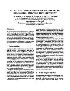
ENERGY-EFFICIENT IMAGE COMPRESSION IN MOBILE DEVICES FOR WIRELESS TRANSMISSION Yamini Nimmagadda, Karthik Kumar and Yung-Hsiang Lu School of Electrical and Computer Engineering, Purdue University, Indiana, USA ABSTRACT This paper presents an adaptive compression algorithm for mobile devices to reduce the transmission energy of images through wireless networks. Our algorithm selects different compression schemes based on the amount of details in the images and the available transmission bandwidths. At low bandwidths, significant amounts of energy can be saved because the reduction in transmission energy outweighs the additional processing energy. We implement this adaptive algorithm on an HP iPAQ hw6945 Personal Digital Assistant (PDA). The algorithm is invoked before transmitting images and is transparent to users. The average energy reduction is 20% with an average delay of 1.1 seconds. 1. INTRODUCTION There has been a dramatic growth in the usage of images in wireless personal communication. Most mobile devices are equipped with digital cameras; users can share their images through wireless networks, including both Wi-Fi and cellular networks. Since wireless mobile devices are battery-operated, transmission energy should be conserved. The transmission energy of images can be reduced by compressing them. However, image compression techniques result in processing energy overhead. It is important to ensure that the processing energy does not exceed the reduction in transmission energy. The wireless bandwidth plays an important role in the selection of the compression parameters. At high bandwidths, images can be transmitted with lower energy consumption; compression energy becomes dominant. At low bandwidths, the transmission energy is higher and can be reduced by better compression with additional processing energy. Several studies [1] [2] have been conducted to select compression parameters based on network bandwidths. These studies assume that all images benefit equally from compression at a given bandwidth. However, some images benefit less than others at a given bandwidth using the same compression parameters. Figure 1 compares two images with resolution 400 × 300 transmitted at a bandwidth as low as 10 kB/s. We use the compression scheme presented in our previous work [3] to compress the images. This figure demonstrates a high energy loss for (a) because the image does not contain fine details. There is no reduction in transmission energy and the processing overhead consumes 0.018 J. Figure 1(c) contains
978-1-4244-4291-1/09/$25.00 ©2009 IEEE
1278
(a)
(b) image (a) (b) (c) (d)
size (kB) 4.2 4.2 16.9 11.6
(c) Et (J) 0.13 0.13 0.27 0.17
(d)
Ep (J)
�E (J)
0.018
-0.018
0.038
0.062
Fig. 1. (a)(c) Original images (b)(d) compressed images using the first scheme. Et : transmission energy. Ep : processing energy. many fine details, including the texture on the floor, walls, and leaves. By removing the textures, 37% transmission energy can be saved with only 14% additional processing energy. The percentages are calculated based on the system energy required to transmit (c). The contributions of this paper are: (1) We analyze the details present in images and decide if the images are good candidates for compression. (2) We provide a framework to select compression schemes based on network bandwidths and the amount of details present in the images. We use two compression schemes: the first scheme is adopted from our previous work [3] that produces high compression ratios and also has high processing energy. This technique is used for images with many fine details. The second scheme is simpler, produces lower compression ratios by averaging intensities of non-edge pixels and has lower processing energy; it can be used for images with fewer details. Figure 2 shows the energy reduction percentages at different bandwidths comparing the first compression scheme and our adaptive algorithm. The graph is obtained by compressing and transmitting 100 images with different amounts of details at different bandwidths. The first scheme can save energy when the available bandwidth is below 45 kB/s. When the bandwidth is higher, the second scheme should be adopted so that energy is not wasted. Our adaptive scheme achieves positive energy savings even at high bandwidths.The bandwidths for the two methods at data points (◦ and ×) do not perfectly coincide due to the variations of the wireless network.
ICME 2009
Percentage Energy Reduction
40 Compression scheme 1
Our adaptive method
30 20 10 0 −10 0
20
40 60 Bandwidth (kB/s)
80
Fig. 2. Percentage reduction of energy for 100 images at different bandwidths. Our algorithm saves energy at all bandwidths.
Fig. 4. Computation of IGT from an intensity histogram. IGT is 25 for this histogram.
Percentage reduction in transmission energy
25 20 15
(a)
10 5 0 2
(b)
(c)
Fig. 5. Images with uniform distribution and different spatial variations: (a) 2.74 kB, (b) 3.22 kB (c) 12.2 kB. 4
6 Entropy
8
10
Fig. 3. Percentage reduction of transmission energy vs. entropy using the first scheme.
compressed using the JPEG standard. This process is invoked before an image is transmitted and is transparent to users.
2. RELATED WORK Several studies have been conducted to reduce the energy for transmitting images over wireless networks. The techniques presented in [1] [2] do not analyze the images before compression and lose energy for processing images with very few details. The techniques in [4] [5] analyze the image but do not consider the effect of network bandwidths on transmission energy. They use Peak Signal-to-Noise Ratio (PSNR), a pixel based quality metric that does not correlate well with the human perception. We use Structural Similarity Index Metric (SSIM) [6] to compare the qualities of original and compressed images. The SSIM is better correlated with the human perception. This paper differs from our previous work [3] in the following ways: (1) This is the first study to analyze contents of images to select compression schemes for different network bandwidths. (2) We implement our algorithm in C# and obtain physical measurement of energy savings and processing time. (3) Users can adjust the qualities of images.
3.1. Estimation of Details We use two metrics namely compressibility index and entropy to analyze the images and select the compression schemes.
3. ENERGY-EFFICIENT IMAGE COMPRESSION Our algorithm has three steps: (1) analyze the image to check if it is a good candidate for compression; (2) if the image needs to be compressed, select one of the two schemes based on the amount of details and the available bandwidth; (3) allow users to tune the quality. We develop a metric called “compressibility index” to check if the image needs to be processed. If the image needs to be processed, we use the entropy of the intensity values of the image to select one of the two compression schemes described in Section 3.2. After an image is processed by our algorithm, the image is further
3.1.1. Compressibility Index Some images cannot benefit from compression because they are composed of regions with same intensity values and without fine details. For example, the size of the image shown in the Figure 1 (a) cannot be reduced. Energy is lost in processing such images. Compressibility Index (CI) checks if the image has fine details before compression to avoid the energy loss. For an image I, the difference D(x, y) at a pixel (x, y) is calculated as follows: D(x, y) = 1, if I(x, y) �= I(x, y + 1) or I(x, y) �= I(x + 1, y) (1) D(x, y) is assigned the value 1 when there is a difference in intensity values between horizontally or vertically adjacent pixels. For images without texture, D is zero for most of the pixels. We now define a value D � (x, y), which is zero when at least one pixel (ˆ x, yˆ) in the neighborhood Rxy is zero. Rxy contains immediate neighbors horizontally, vertically and diagonally to the pixel (x, y). If there are no zeros, the intensities of pixels are different from one another. CI is the summation of values of D � over all the pixels in the image. If CI = 0, the images have large regions of pixels with same colors and we transmit the original JPEG images. If CI > 0, we calculate the entropy of the image to select the compression scheme. 3.1.2. Entropy The amount of details in an image is estimated before selecting one of the two schemes. This estimation must have low
1279
3.2.2. Color Averaging The second compression scheme averages colors of blocks of pixels. Averaging is a widely used technique for smoothing images. This technique reduces image sizes by removing fine color variations. The images look blurred after averaging because colors smear across the edges. We improve averaging by detecting the edges of the image and averaging only the non-edge pixels. We use a 3 × 3 window for averaging the pixels because larger window sizes result in blurred images. 3.3. Selection of Compression Schemes 3.3.1. Energy Model Our algorithm selects one of the two compression schemes described in Section 3.2 based on two factors: an image’s entropy and the available bandwidth. The baseline is to transmit the image directly. Let Et be this baseline transmission energy, measured from the transmission power Pt and the transmission time Tt . The energy consumed by our algorithm can be divided into three parts: (1) the decision energy, (2) the processing energy, and (3) the transmission energy. Etotal = Ed + Ep + Et� = Pd Td + Pp Tp + Pt Tt� .
(2)
1280
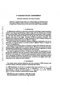
(b) (21,13,0.84) (c) (50,12,0.79) (d) (100,11,0.7)
Fig. 6. Images compressed using various IGTs. The triplets represent IGT, size (kB), SSIM. Energy normalized to original transmission energy
3.2. Compression Schemes 3.2.1. Detail Removal The first compression scheme [3] has three steps: continuous edge detection, image segmentation, and intensity normalization. The first step detects the boundaries of objects ignoring fine details by using a parameter called “Intensity Gradient Threshold” (IGT). IGT is measured from the image’s intensity histogram as the smallest difference between the peaks (peaks correspond to large regions with similar colors). Figure 4 shows an example of computing IGT. The edge image is used to segment the image into regions containing similar colors. In the intensity normalization step, the mean intensity value of each segment is computed, and the non-edge pixels are assigned the mean value (edge pixels are not used to preserve their sharpness).
(a) (0,17,1)
100
Et Ep Ed δE
80 60 40 20 0 From 25 Histogram
50 IGT
75
100
Fig. 7. Energy distribution for various IGTs (The energy is normalized to the baseline transmission energy, higher �E is better). where Ed is the decision energy measured from power Pd and time Td required to select the compression scheme. Ep is the processing energy measured from power Pp and time Tp . Et� is the transmission energy measured from power Pt and time Tt� required to transmit the processed image. The energy savings �E is the difference between the total energy of our algorithm and the baseline energy: �S − P d Td − P p Tp , (3) �E = Etotal − Et = Pt Ba where �S is the reduction in the image size, and Ba is the available bandwidth. From Equation (3), the energy reduction is affected by the reduction in image size and the available bandwidth. 3.3.2. Selection Threshold We compute the entropy of a JPEG image and compare it with a threshold T h to choose a scheme. If the image’s entropy is above the threshold, the first scheme is chosen. Otherwise, 0.2
Energy Savings (J)
overhead. We use entropy to determine the amount of details in images. When an image has a high entropy, it has more details and a greater potential to achieve a higher compression ratio. An image with a low entropy has fewer details and cannot benefit from the first compression � scheme. The entropy E of image I is defined as E = − 0≤i≤2b −1 p(i)log(p(i)), where p(i) is the probability of the intensity value i, and b is the number of bits per pixel per color. For a given color image, the red, green, and blue colors have 2b possible values each. If an image has few details, the entropy is low and the second scheme should be used to save energy. If an image contains many fine details, its entropy is high and can achieve a high compression ratio when the first scheme is used. Figure 3 shows higher reduction in transmission energy for images with high entropy values.
anisotropic gaussian EEWITA Low−pass filter Taylors JPEG Adaptive Rendering
0.15 0.1 0.05 0 20
40 60 80 Bandwidth (kB/s)
100
Fig. 8. Comparison of energy savings averaged over 100 images for different techniques.
the second scheme is used. We propose an empirical formula a to compute the threshold T h = αB S , where α is a constant and S is the size of the original JPEG image. The constant α is obtained by considering images that have same intensity distribution, but different spatial distributions. Figure 5 shows three images with the same intensity distribution, but different spatial distributions: (a), (b) and (c) are compressed to 2.74 kB, 3.22 kB, and 12.2 kB respectively by JPEG. We experimentally find that the energy reduction obtained by compressing the images (a) and (b) is negative above 47 kB/s and 64 kB/s respectively using only the first compression scheme. The image (c) always shows a positive reduction in energy, because the Wi-Fi bandwidth available is sufficient to obtain positive energy savings. We do not consider this image for the calculation of α. All three images have an entropy value of E0 = 5.542. The entropy constant α for the images (a) and (b) are 0.32 and 0.28 respectively. We use images with different resolutions, intensity and spatial distributions and observe that α approximates to 0.3. 3.4. Quality and Size Trade-off In the first compression scheme, the parameter IGT determined from the histogram maintains acceptable image qualities. We explore the variation of image sizes and qualities with the variations in IGT, and allow users to control compression ratios and qualities. Higher compression ratios can be achieved by increasing IGT; meanwhile, image qualities degrade. When IGT increases, more pixels are grouped into a segment, resulting in lower mean intensity values. This process may merge segments corresponding to different objects, degrading the image quality. At a smaller IGT, fewer pixels are grouped into a segment. This may separate segments corresponding to the same object, preserve the fine variations, and enhance the image qualities with a larger image size. 4. EXPERIMENTS 4.1. Experimental Setup We implement our algorithm in C# on HP-iPAQ hw6945 PDA. The current drawn by the battery is obtained by measuring voltage values across a 0.25 Ω resistor. The values are read by a National Instruments data acquisition card installed on a separate computer at a sampling frequency of 10 kHz. This setup measures the system power, including the display, the processor, and the wireless network interface. The images are transmitted from the PDA to a web server through a Wi-Fi network. We use 100 images including people, objects, and outdoor scenes obtained by using a 3MP digital camera and resizing to 400 × 300 with ImageMagick. 4.2. Energy Reduction The energy savings are calculated by using Equation (3). Our adaptive algorithm achieves energy savings across a wide range of the network bandwidths for all 100 images, as shown in Figure 2. Our method obtains 20% average energy reduction, including 35% reduction in transmission energy and 15% additional processing energy. The average energy
1281
reduction (obtained from averaging energy reduction over all the images and at various bandwidths) using only scheme 1 is 13%, using only scheme 2 is 9%, using our adaptive scheme is 20%. The percentages are calculated based on the energy to transmit the original JPEG files. Figure 6 shows the images compressed using various IGTs. Figure 6(a) shows the original image (size: 16.9 kB); (b) shows the image compressed with IGT computed from the intensity histogram (size: 13.3 kB); (c), (d) show images compressed using IGT values of 50 and 100 respectively. The quality is measured using SSIM. As IGT increases, the compression ratio increases, but the quality degrades (lower SSIM values); higher color dispersion is observed in (d). Figure 7 shows the distribution of energy for decision, compression and transmission steps of our method. The energy is normalized to the baseline transmission energy. As we increase IGT, the maximum energy reduction obtained is 39%. The processing energy varies slightly with IGT, because of the variations in the formation of segments and thereby the number of comparisons. Figure 8 shows the comparison of energy savings averaged over 100 images using different compression techniques. The techniques used for comparison include basic smoothing algorithms like Gaussian filter, lowpass filter, and anisotropic filter and also adaptive JPEG [1] and wavelet [2] mentioned in Section 2. Our method achieves positive energy reduction even at high bandwidths. 5. CONCLUSION We present an adaptive image compression algorithm to save transmission energy through wireless networks. This method achieves 20% energy reduction on average. This is achieved by 35% reduction in transmission energy with 15% additional processing energy. We allow users to tune the image qualities and sizes. Acknowledgments: This project is supported in part by NSF CNS-0347466 and CCF-0541267. Any opinions, findings, and conclusions or recommendations in the projects are those of the investigators and do not necessarily reflect the views of the sponsors. 6. REFERENCES [1] C. Taylor and S. Dey, “Adaptive Image Compression for Wireless Multimedia Communication,” ICC, 2001. [2] Dong-Gi Lee and Dey, S., “Adaptive and Energy Efficient Wavelet Image Compression for Mobile Multimedia Data Services,” ICC, 2002. [3] Yamini Nimmagadda, Yung-Hsiang Lu, Edward J. Delp III, and David S. Ebert, “Non-Photorealistic Rendering for Energy Conservation in Portable Devices,” in Electronic Imaging: Multimedia on Mobile Devices, 2008, vol. 6821. [4] Kewu Peng and John C. Kieffer, “Embedded Image Compression Based on Wavelet Pixel Classification and Sorting,” IEEE TIP, 2004. [5] Hing T Xiangjan He, Huaqing Wang and Namho Hur, “Fractal Compression on Spiral Architecture,” CGIV, pp. 76–83, 2006. [6] Zhou Wang, Alan C. Bovik, Hamid R. Sheikh and Eero P. Simoncelli, “Image Quality Assessment: From Error Visibility to Structural Similarity,” IEEE TIP, vol. 13, no. 4, 2004.