Enforcing Security with Behavioral Fingerprinting J´erˆome Franc¸ois, Radu State, Thomas Engel
Olivier Festor
SnT – NetLab – University of Luxembourg Campus Kirchberg, L-1359 Luxembourg Luxembourg {firstname.lastname}@uni.lu
INRIA Nancy Grand Est - Madynes 615 rue du Jardin Botanique 54600 Villers-l`es-Nancy France
[email protected]
Abstract—Although fingerprinting techniques are helpful for security assessment, they have limited support to advanced security related applications. We have developed a new security framework focusing especially on the authentication reinforcement and the automatic generation of stateful firewall rules based on behavioral fingerprinting. Such fingerprinting is highly effective in capturing sequential patterns in the behavior of a device. A new machine learning technique is also adapted to monitor high speed networks by evaluating both computational complexity and experimented performances.
I. I NTRODUCTION Fingerprinting automatically infers specific information from monitored devices: operating system [1], [2], protocol used [3] or device type [4], [5], [6] (or protocol stack). The latter infers automatically the types of devices: brand name, series of hardware or name and version of software. Such tools are helpful for security assessment by revealing devices having security flaws in a network like for instance operating systems or software having known vulnerabilities. Moreover, an attacker can hide itself by spoofing normal device type. To detect that, our approach takes benefit from our previous fingerprinting method [4], [6] which characterizes a device by its behavior i.e., the way it interacts with others. This kind of fingerprinting can also catch attack behaviors to create automatically attack patterns which might be inputted as signatures for an Intrusion Detection System (IDS). However, a main issue is the real-time applicability of such techniques for safeguarding efficiently users, hosts and network infrastructure. Thus, the contribution of this paper is threefold. Firstly, a new method is proposed for managing behavioral fingerprints. Secondly, we propose the Behavioral Security Framework using fingerprinting for security purposes like vulnerable device discovery, spoofing detection or automated attack signature creation. Finally, complexity issues are evaluated analytically and experimentally. Regarding our previous work [4], [6], we have reused the construction of the behavioral fingerprints as well as the SVM classification. This paper is structured as follows. The framework is described in section II. Section III details the fingerprinting technique. The security applications are assessed in section IV as well as the complexity in section V. Section VI highlights main related work. Conclusion is given in section VII.
II. F INGERPRINTING
BASED SECURITY FRAMEWORK
The Behavioral Security Framework depicted in figure 1 is based on behavioral fingerprinting. This paper introduces two main applications: authentication reinforcement (authentication module) and attack/intrusion detection (attack module), and voluntary omits applications related to security vulnerabilities assessment based on a general inventory of connected devices, which may be directly derived from fingerprinting [5]. Figure 1 shows the architecture including a first level of protection (firewall and/or an IDS) screening the traffic as a first step towards a more rigorous authentication. A. Authentication reinforcement The first module of our security framework reinforces the user authentication. Obviously, the latter cannot be exclusively based on fingerprinting but should use an authentication mechanism such as password protection or certificate based solutions but they are still faced with security issues. For example, stealing passwords using a dictionary, social engineering or phishing is easily possible [7]. Thus, device fingerprinting is helpful in detecting an anomalous device type even if the user succeeds to authenticate. Anomalies could be related to attacker activities but can also reflect a normal behavior change. Therefore, the authentication module within the behavioral security framework (figure figure 1) only provides results to the original authentication module responsible to trigger counter-measures. For example, if the fingerprinting detects an anomaly, the user could be required to do an additional check (second password, email confirmation, usage of a TLS certificate, alarm reported to the administrator...). Moreover, if the second check succeeds, the user profile has to be updated. In fact, anomalies might be detected in parallel in two manners. On one hand, a difference between the announced type, since most of protocols define a user agent field [8], [9], and the type automatically inferred can be detected. The attackers, who execute specific tools, prefer to announce faked user agents for avoiding detection (type spoofing) since they often specific tools. Thus, the first authentication reinforcement has to compare the inferred device type by fingerprinting with the announced device type. On the other hand, the user behaviors may be monitored over time to profile the types they use and track deviations from them.
Restricted users Network
Protected Network
Internet Firewall
Authentication
Behavioral Security Framework Authentication Module Device identity inference User agent deviation Long monitoring deviation
Attack Module Attack monitoring
(a) Twinkle 1.10 (softphone)
(b) Cisco 7940 (hardphone)
Stateful rule generation
Fig. 2: TR-FSM examples. Two shared paths are grey colored Fig. 1: Behavioral security framework
uu u t t t t t tt u uu t u x xx x x x x xxxx x x xx x xx x x x o o oo oo o x o o oo
B. Attack module The attack module (figure figure 1) might be trained with attack generators such as KiF [10], which produces and discovers automatically new attacks for SIP [8] (Session Initiation Protocol). The fingerprint of the attacks can then be automatically generated and expressed with stateful firewall rules. If the firewall is able to filter the traffic regarding such rules, its configuration is updated, otherwise it has to delegate the process to the attack module itself which will then only output the action to trigger. Otherwise, the attack module can be trained with normal behaviors to act as an anomaly intrusion detection system by looking for behaviors too much divergent from a profile. III. B EHAVIORAL F INGERPRINTING Behavioral fingerprinting was introduced in [6]. The key idea is to represent the devices by their behaviors: the way they interact with other ones. Since the original work includes all theoretical details, this section gives an overview and provides some extensions: a new technique based on K-TRACE and the definition of the result confidence. A. TR-FSM model The behavior of a device type is represented as a Temporal Random Parameterized Tree Extended Finite State Machine (TR-FSM) and corresponds to the manner a device sends the requests and how it replies to the requests from other ones. Moreover, the behavioral fingerprinting takes in account the message delays. A TR-FSM is a tree based representation of the device specific protocol state machine including delays as shown in figure 2. In fact each node represents the type of the message which is emitted (prefixed by !) or received (prefixed by ?). An edge between two nodes indicates that they have been successively monitored in the same session. The delay between them is put as an attribute on the edge. Basically, for each observed sequence of messages, a branch is created. Then, the branches are aggregated using a generic root node and the common prefix are merged such as the node !INVITE in figure 2(a). The protocol knowledge is reduced to the message types, which can be automatically inferred as highlighted in [6] or based on a message parser. It eases the applicability of our
Medoids method
Nearest Neighbors
Fig. 3: Common classification problems
behavioral security framework to any protocol. Furthermore, the time measurements are dependent of the network locations. Hence, the round-trip time has to be measured and filtered out. Otherwise, if the measurements are always done at the same location, this step can be avoided. B. Classification Once the TR-FSMs are constructed, they have to be classified. Support Vector Machines (SVM) are good trade-offs between accuracy and computational complexity [11] and have proved their efficiency[6]. To extend the evaluation, this paper introduces another method, TRACE/K-TRACE [12], which is, like SVM, dedicated to separate data points which are not linearly disjoint and we propose a very low computational version hereafter. The limited overhead is also highlighted in our evaluation while the accuracy is not degraded. A common classification problem with non linearily separable data is depicted in figure 3 where traditional clustering methods fails to separate the different clusters. 1) SVM: Supposing P different kinds of devices which form the set D = {d1 , . . . , dP }, L = {l1 , . . . , lM } is the training set of M TR-FSMs. Multi-class SVM resolve optimization problems to determine separating hyperplanes in a higher dimensional space where points have been projected using a function φ (figure 4), and with maximum margins for each pair of classes (types). Hence, assuming two types, dl and dk , the hyperplane hlk is characterized by a subset of points of L, namely support vectors, SV lk , belonging to type dl or dk . The decision function is directly derived from these supports vectors. Thus, flk (tx ) returns the predicted type for tx
x x xx xx
x xx oo o o ooo x xx ooo o x TRACE
$
SVM
x xx xx x xx x x x xx
o o oo ooo o ooo
S = {ti |∃blk , bsr , ti ∈ clk , d(ti , bsr ) < d(ti , blk )}
KTRACE
x x xx xx
x xx oo o o ooo x xx ooo o x
3) selects all points whose the closest barycenter is not the one of the corresponding class:
$
x x x xxxxxx $
xx xx
oo o ooooo o oo
Fig. 4: Machine learning methods and non linearly separable data points (2 classes). SVM finds a separator after projection. TRACE discovers barycenters of each cluster. K-TRACE projects points into a higher dimensional space for reducing the number of clusters. A new point, $, is assigned depending on its position regarding the hyperplane (SVM) or to the closest barycenter (TRACE and K-TRACE)
regarding hlk . This corresponds of the side-position of a point to assign, $ in figure 4. Since there are several hyperplanes (one per pair of types), the predicted type corresponds to mostly chosen one by all the decision functions. As defining the projection function φ is hard, a kernel function is applied to a pair of points, K(ti , tj ), and has to follow strong properties [13]. Details may be found in our prior work [6] proving the correctness of a TR-FSM based kernel function which mainly relies on counting the number of common paths (sequence of nodes from the root to any other node) weighted by the delays. 2) K-TRACE: K-TRACE [12] is a kernel-based extension of the Total Recognition by Adaptive Classification Experiments (TRACE). TRACE algorithm is executed in a supervised manner and is well suited for piece-case linearly separable data points for which traditional clustering methods fail because they look for continuous clusters. To discover the multiple clusters corresponding to a single class (device type), TRACE finds multiple barycenters (figure 4) thanks to a learning process (also called training). The initialization creates one cluster per class containing all points from L of this class. Hence, the set C = {c11 , . . . , c1P } is built from the trees ti of the training set: c1j = {ti |real(ti ) = dj }
(1)
where real(ti ) returns the real identity of a tree in the learning set L. Actually, cji represents the j th clusters of the type i. Then, the algorithm computes the barycenters of the clusters and divides a cluster in case of incoherency, i.e. the closest barycenter from a point is not the one of its own cluster. More precisely, it works as follows: 1) compute each barycenter, B = {bji }, for each cluster cji of C 2) compute all Euclidean distances d(ti , blk ) for all ti belonging to the training set and all blk in B
(2)
4) stop if S is empty 5) select the tree of S, b+ , which is the farthest from its barycenter: 6) get all the clusters, C ′ , containing points of the type real(b+ ) 7) apply k-means on C ′ by using the original barycenters and b+ as seeds. As K-means is usually employed with unlabeled data, the seeds are randomly selected unlike our approach. In this case, our approach and its evaluation is not dependent on a specific initial configuration. 8) since a new barycenter is added, a new cluster of the same type (real(b+ )) is created. The set C is updated with the constructed clusters by k-means 9) go to step 1 The testing stage is based on the final set of barycenters B. In fact, each new point to identify is affected to the type corresponding to the closest barycenter (figure 4). Applying a projection function, like SVM, helps to increase the separability of the points and so to reduce the number of TRACE iterations and the set of final barycenters, which speeds up the classification during the testing stage. This algorithm, K-TRACE, is a kernel-based method and is depicted in figure 4. Therefore, the algorithm is exactly the same than TRACE but it is executed on the projected data points φ(ti ). Similarly to SVM, the definition of this function is not straightforward and justify the use of the kernel trick: K(ti , tj ) = h φ(ti ).φ( tj ) i. However, the Euclidian distance normally based on φ(ti ) has to be computed as follows between ti and the barycenter blk : d(ti , blk ) = K(ti , ti )−
2 X 2 X X K(ti , x)+ l 2 K(x, y) l |βk | |βk | l l l x∈βk
x∈βk y∈βk
(3)
with: βkl = {ti |ti ∈ clk }
(4)
Identifying a new device representation needs to compute its distance from all barycenters and so from all other data points from the training set as shown in equation (3). Thus, the complexity is very high whereas the goal is to speed up the classification. Consequently, we propose a simple adaptation to keep the original interest of TRACE by representing each subcluster by an unique point. In fact, the closest point of each computer barycenters during the training stage is kept. They form the set B ′ .Then, the distances between a new tree, tx , to classify and each of them, tj , is computed in the higher dimensional using the kernel function similar to [12]: d(tx , tj ) = K(tx , ti ) + K(tj , tj ) − 2K(tx , tj )
(5)
Unlike equation (3), the calculation does not require to compute the kernel functions with all other points of the cluster.
C. Confidence level Security applications usually rely on confidence levels in order to trigger correct counter-measures without blocking too many normal connections (false positives). Thus, we propose in this section a way to determine the confidence level of the predicted type. Assuming the TR-FSM tx , it is assigned to the type d = assigned(tx ) based on several decision functions using SVM. In fact, the sign of flk (tx ) indicates if the device tx belongs to the type l or k. Then the class which is mainly chosen is considered as the good one. Considering the distribution |{fdp , fdp (tx ) > 0}| V (tx = dp ) = , the identification result |{flk }| d corresponds to arg max V (tx = dp ). In fact, the distribution k
represents the proportion of voters for each possible device type. Hence, the value V (tx = d) helps to determine the confidence level. The result should have more impact if the vote is not floating. A floating vote result is equivalent to a low standard deviation. Considering σV as the standard deviation of the distribution V , the confidence level is defined as follows: c(tx ) = α × V (tx = d) + β × σV
(6)
α and β can be tuned. In this paper, they are fixed to 0.5 for computing the usual mean. Regarding K-TRACE, the higher the difference between the distance from the closest barycenter to the point to assign and the distance from others, the higher the confidence should be. So, to keep the same definition as prior, the distances are normalized between 0 and 1 and the following distribution is defined: 1 − minl d(tx , blp ) V (tx = dp ) = P l bl 1 − d(tx , bk ) k
This refined distribution definition is then used in (6). IV. E VALUATION The experiments are based on SIP [8] which is well used by VoIP operators since it is designed for managing multimedia sessions. Due to its popularity, a broad range of VoIP threats appeared last years [14] whereas it becomes one major service in the Internet. Therefore, designing efficient solutions for VoIP service is necessary but the approach described in this paper remains generic. A. Accuracy assessment Our evaluation is based on the same datasets than in [6] (table I)) with network traces from our own testbed and also from a real VoIP operator (T1, T2) that we assume originally free of attacks. 40% of the data were used for training the system with the testbed dataset because of its relative small size, although we have evaluated our system in a critical way when using real data as only 10% have been used during the training. In addition, each experiment is run ten times where message sequences are shuffled prior. General statistics about the datasets and fingerprinting accuracy are given in table I. Regarding our context, the accuracy
#device types #messages Avg packet size (#bytes) Avg. TR-FSM size (#nodes) %learning avg SVM Accuracy std avg K-TRACE Accuracy std
Testbed 26 18066 541 18.97 40 0.91 0.011 0.84 0.032
T1 40 96033 465 12.93 10 0.81 0.004 0.73 0.008
T2 42 95908 466 12.94 10 0.86 0.002 0.74 0.005
TABLE I: Experimental datasets fingerprinting results
Min. confidence of right identification Max. confidence of wrong identification
Testbed 0.56677 0.56658
T1 0.54706 0.54410
T2 0.54580 0.54153
TABLE II: Maximal and minimal confidence levels
is the proportion of devices which are assigned to the correct types. Assuming a set P of N predictions represented as predij meaning that a prediction of type j was made for a device of real type i, the accuracy is: P predij ∈P,i==j 1
N Performances are better with the testbed dataset because the learning is executed on a bigger proportion of data. The operator dataset includes some device types under represented, which leads to degrade the results. Moreover, K-TRACE is less accurate but is still acceptable since the accuracy varies between 0.73 and 0.84 depending on the dataset. The standard deviation highlights that results are quite stable. Hence, as it is claimed in this paper, this proves that fingerprinting can enforce security applications but have to be carefully taken in account due to the errors entailed by classification techniques. Additional results about SVM and the tuning of parameters (especially the number of message sequences to use) can be found in the original paper [6]. B. Calibration The following experiment evaluates the confidence level described in section III-C in two ways: when the identification is right or when it is wrong. The goal is to calibrate the system and to define a threshold τ evaluating the correctness of the identification: a confidence level lower than τ indicates that the result needs to be considered carefully. Due to space constraint, this section presents SVM-based results but conclusions are identical for K-TRACE. After running multiple experiments and calculating the average confidence levels for right and wrong results, the minimal and maximal values can be computed as shown in table II. It shows that the minimal average confidence for a correct identification is always greater than the maximal average confidence of wrong identifications. The confidence level of the right and wrong identifications have close average confidence levels (around 0.56665) for the testbed dataset and with a standard deviation of 0.00005. This experiment helps to determine the threshold τ which can be set for example to the average between the two values represented.
Fig. 5: Intrusion detection based on fingerprinting 0.7
0.3 0.2
0
True positive rate
0.8 0.6 0.4 0.2 0
1
09
0.
08
0.
07
0.
06
0.
05
0.
04
0.
03
0.
02
0.
01
0.
TABLE III: Attack traffic statistics
3
1
0.
#call initiation 27 19 21 64
1 2 Alert level
Fig. 6: Traffic distribution regarding the alert levels
0
#sessions 18 18 16 40
0.4
0
Attackers use specific tools not used by legitimate users. Hence, they masquerade as legitimate device types. Figure 5 summarizes the functioning of the detection. In fact, each device announces its type (user-agent) which is compared to the fingerprinting result. However, due to fingerprinting errors, the confidence level is taken in account. Hence, when the confidence level is high, a similar announced and fingerprinted type implies no alert (level 0) whereas a divergence is synonym of an intruder pretending to be another kind of device (maximal alert level). When the confidence level is not high, the decision strength is lower and then alert level is one when the identity does not diverge and two otherwise. Attack traffic was generated on the testbed using the bot presented in [15] generating phone calls. The bot pretends to belong a known device type from the training set. Table III highlights the statistics from the attack traffic generated. The traffic from the bots is mixed with 60% of the normal traffic. τ is set to 0.5667 as it is an intermediary value highlighted on table III. The distribution of benign and attack traffic regarding the alerts is represented on figure 6. The benign traffic entails many alerts of level zero and one whereas the attack traffic is split into level two and three. Therefore, the attacks are clearly distinguishable even if ten percents of the benign traffic is about equally divided into alerts level two and three. However, no attack has an alert level lower than two. The ROC (Receiver Operating Characteristic) curve is plotted in figure 7 by varying τ . Only the identifications having a confidence higher than τ are plotted (true or false positives). The scale highlights a huge increase of the true positives rates comparing with the false positives since detecting 100% of the attacks implies ten percents of false positives. Thus, if the system triggers an additional check for a priori malicious #msgs 220 197 150 432
0.5
0.1
C. Authentication reinforcement
Device type SJPhone v1.65 Cisco 7940-v7 Snom v5.3 Twinkle v1.1
Attack trafic Benign trafic
0.6 Proportion of traffic
For example, τ = 0.5456 is suitable for the dataset T1. In this case, only right identifications are kept. Hence, the proposed confidence level definition clearly improves the viability of fingerprinting for supporting security applications. Choosing always a high threshold, close to the maximal observed values for the correct identifications, is another possible choice to be very cautious.
False positive rate
Fig. 7: User agent masquerading detection - ROC curve
users, ten percents of normal users will be affected. Using K-TRACE, the results are affected in a similar way than in section IV-A. Training the system with attack tools implies that 99.1% of them are directly detected afterwards with a high confidence value (higher than 0.5667 for SVM, which is the previously determined value) whereas the normal traffic is never considered as an attack. D. Attack detection Automated learning of stateful firewall rules is one of the main application of the attack module of our behavioral security framework. In fact, stateful firewall rules can be directly generated from the TR-FSM of an attacking device. The attack is run multiple times in order to collect several possible sessions which are aggregated into a TR-FSM. Figure 8(a) represents the results from a denial of service attack reported in CVE (Common Vulnerabilities and Exposures) 2007-4459 against a Cisco 7940. The attack uses only ten messages and the device responses are often errors (400, 404) due to the invalidity of the requests. Each individual message is legitimate and thus a simple signature detection will not discard it. Therefore, only the global sequence of sent messages can achieve the attack.
5e-05
0.4
4e-05 time (s)
time (s)
0.5
0.3 0.2
3e-05 2e-05
0.1
1e-05
0
0
00 28 0 0 26 0 0 24 0 0 22 0 0 20 0 0 18 0 0 16 0 0 14 0 0 12 0 0 10 0 80 0 60
00 12 00 11 00 10 0 90 0 80 0 70 0 60 0 50 0 40 0 30 0 20 length(message)
length(message)
(a) Syntactic parsing
(b) Direct access
Fig. 9: Computation time for recovering the message typ regarding the length of the message
Fig. 10: Running time for TR-FSM comparison regarding the cardinality of trees
device behavior along its lifetime. The first step defines the events ev_Invite and ev_Options corresponding to the different kinds of emitted messages (INVITE and OPTIONS): definition SIPMessages begin when SIP:request.method @ match "ˆINVITE" -> let: event ev_Invite; when SIP:request.method @ match "ˆOPTIONS" -> let: event ev_Options; definition end
Then, the attack is described as a sequence of events (regular expressions are authorized) equivalent to the messages in figure 8(b): veto attack_cisco uses SIPMessages begin (ev_Invite,ev_Options[*2],ev_Invite,ev_Options[*3], ev_Invite,ev_Options[*2]) -> drop; veto end
(a) TR-FSM of the attack
(b) rule
Stateful
Fig. 8: Generation of the stateful rule of the attack against Cisco Phone 7940
Because responses are not defined as events, they are ignored by SecSip. Hence, when the previously defined sequence of events is detected, the message corresponding to the last event is dropped to stop the attack. For improving the detection, the delays can also be included in VeTo rules. Including delays in stateful rules is a user choice but can be clearly an added value for a certain kind of attack like flooding attacks as SpIT (Spam over Internet Telephony) can be. Obviously, this attack is a simple example to illustrate the process and the rule could be created easily by hand but more complex attacks can include many messages sequences (alternative paths in the tree) for which an automatic tool such as proposed in this section is required. V. R EAL - TIME APPLICABILITY
Then, the TR-FSM can be considered as a stateful rule for a firewall but it can be restricted to messages from the attacker (prefixed by !) for discarding the normal device behavior. For example, if an attacker tries this attack on many devices without knowing their real types, the responses sent can differ but not the attack messages. Moreover, building several TR-FSM with different devices allows to construct a more complete stateful rule. Thus, by removing responses from figure 8(a), all branches are identical and composed of INVITE and OPTIONS in the same order leading to aggregate them into a single sequence based signature depicted in figure 8(b). This rule is injected into SecSip, a stateful firewall [16] based on a new language, VeTo[17], for tracking SIP
For assessing the real-time applicability, this section includes analytical facts as well as experimental results based on a single computer (Intel Core 2 Duo 3GHz). A. Message parsing The first task is to determine the types of the messages when building a TR-FSM. Thus, the complexity is highly dependent on the protocol grammar and a straight-forward manner is to parse entirely the message to construct its syntactic tree as also used for device fingerprinting in [5]. However, the type is generally a field which is identified by a certain keyword or a certain position and so it can be easily found without constructing the complete syntactic tree: direct access to the
Stage Parsing Tree construction Tree comparison
Execution time (seconds) 25% percentile median 75% percentile 1.001 × 10⁻⁵ 1.097 × 10⁻⁵ 1.192 × 10⁻⁵ 1.597 × 10⁻⁵ 2.384 × 10⁻⁵ 3.409 × 10⁻⁵ 1.097 × 10⁻⁵ 2.694 × 10⁻⁵ 5.198 × 10⁻⁵
complexity
regression
Constant O(#messages) O(#nodes × #nodes)
y = 1.087 × 10− 5 y = 9.911 × 10⁻⁷ x + 1.478 × 10−06 y = 5.348 × 10−7 x2 + 2.033 × 10−05
TABLE IV: Performance evaluation
B. TR-FSM construction Constructing a TR-FSM is divided in two times: (1) message sequences must be monitored and (2) have to be aggregated to build a TR-FSM. The running time of the first step cannot be avoided but also dependent on the network throughput and the device activity. So, associating a complexity to this one is meaningless. However, the second stage has to agglomerate such messages into a TR-FSM which implies a linear complexity regarding the total number of messages composing the tree [6]. This is checked in table IV. Fortunately, the entire TR-FSM construction is very fast with a median value equals 0.024 ms (table IV). C. Machine learning By design, the kernel function computation requires to compute the intersection between paths of the trees to compare. From an analytical complexity point of view, this is equivalent to compare syntactic trees [5] except that timing differences are also computed, i.e. the complexity is quadratic with respect to the number of nodes. This is confirmed in figure 10 and in table IV. K-TRACE and SVM both iterate multiple times to find a way to separate data points. Hence, the computation time of the training stage is highly dependent on the data (separability of data points) and the initialization of the SVM related optimization problem. Furthermore, evaluating precisely the complexity of this stage is not the most important since it can be done offline and only the identification itself (testing stage) has to be done online. However, our experiments show that the learning time is not the bottleneck (maximum one hour for a daily update). The main advantage of the learning techniques is to extract a subset of training data points which will be then compared
5.5
Reduction factor
position in the message or one of the first parsed fields as for instance in SIP. This implies a constant complexity since the type is given by few bytes encapsulating in a small range of the first bytes. In contrast, a syntactic parser able to deal with huge grammars presenting potential ambiguities [18], [19] is known to have a linear complexity in most cases. We present results of evaluating the time to parse the messages and to retrieve the necessary information in figure 9. For most cases, the time function follows the theoretical complexity mentioned previously but highlights an incompressible time equivalent to 13,1 milliseconds (intercept) if the complete syntactic tree is built, although that the time for a simple parsing is well concentrated around the median value (1.097 × 10⁻⁵ seconds) as shown in table IV. Hence, syntactic fingerprinting as proposed in [5] is not suited to the context of high speed monitoring.
SVM 5 KTRACE 4.5 4 3.5 3 2.5 2 1.5 1 0
20
40
60
80
100
%training
Fig. 11: Reduction factor with different training set size
to a new point to classify, i.e., a new device. SVM returns a set of NSV supports vectors and K-TRACE, a set of Nbary points representing the barycenters (see section III-B for details). The time for identifying a device is directly dependent on them because they correspond to the number of comparisons to perform. Considering Ntrain the number of samples in the original training set, the reduction factor is defined as: Ntrain if SV M NSV reduction f actor = N train if K − T RACE Nbary
The less efficient the training is, the lower this factor is (minimum is one). This factor is plotted in figure 11 and increases while the learning percentage also. Actually, when trees are added to the training samples, the probability to have redundant information, i.e., similar trees, increases also. Thus, more trees will be discarded and the reduction factor is better. Figure 11 highlights the great efficiency of the K-TRACE method comparing with SVM. Thus, K-TRACE is more capable to discard redundant information when the training set is expanded although SVM kept most of points as shown by a reduction factor close to 1.
D. Identification time Assuming tparsing , the time for parsing a message, tbuild , the time for constructing a TR-FSM and tcomp the time for comparing two TR-FSMs, the total execution time of one online identification is: t = tparsing × card + tbuild + tcomp × Nsamples where card is the average number of nodes in a TR-FSM and is varying depending on monitored sessions. Hence, the global time corresponds to parse the different messages, to construct the TR-FSM and finally to compare this tree with
Identification time (s)
1
Worst case Avg.
0.1 0.01 0.001 0.0001 1e-05 1
10
100
1000
10000
#selected training trees
Fig. 12: Online identification time
previously selected training trees. In order to keep pace with the network throughput, a device has to be identified before the next identification starts which means that t ≤ inter packet time × card where inter packet time is the inter arrival time between two packets. Hence, we obtain: tcomp tbuild + × Nsamples ≤ inter packet time card card The different terms of this equation depend on the protocol and the user activities. The operator and the testbed network are similar in terms of TR-FSM sizes and message lengths (table I) which are the main factors impacting the computation time. Hence, regression functions in table IV can be considered for extrapolating the results to the operator dataset. Therefore, figure 12 displays the global computation time depending on the number of selected TR-FSM (NSV or Nbary ) and the average value for card (table IV) together with the worst case when card = 1. The operator dataset (T1) has an average throughput of 110 messages per second equivalent to 9 milliseconds between two messages and so excludes the SVM method because the training process selects more than 10,000 NSV (support vectors) whereas K-TRACE computes about 110 distinct Nbary (barycenters) which is acceptable (figure 12). In this case, fingerprinting requires around 0.2ms per packet which corresponds to a maximal network througput of 5000 packets per second. Considering the statistics in table I, this is also equivalent to 2.2 GB/second. Assuming our configuration and the same reasoning, SVM, which provides the best accuracy, is only viable if the througput for SIP is lower than 21 MB/second. tparsing +
VI. R ELATED WORK There are different kinds of fingerprinting methods. Passive techniques only monitor the devices like p0F [1] which aims at finding the operating system. NMAP [2] uses active techniques i.e., probing the devices with specific requests. Although there are different levels of granularity (operating systems: [1], [2]; protocol: [3]; device type: [20], [4]), none of them are leveraged for advanced security purposes especially device type fingerprinting. The behavioral fingerprinting was introduced in [4], [6] and does not require a full syntactic [5] or semantic [21] knowledge about the protocol. As argued in this paper behavioral fingerprinting can be easily extended to security purposes. IDS research has skyrocketed in parallel of the Internet. Different surveys, as for example [22], highlight the two main classes of IDS. Signature based IDSs such as Snort [23] identify an attack based on a
signature. Anomaly based IDSs detect an attack based on its deviation from a normal profile. Such systems have a higher ability to detect unknown attacks but the number of false positives is higher. Hence, the trend is to use more and more sophisticated techniques as for example [24]. Obviously, the idea of modeling behavior was explored in the past. User behavior was generally modeled as its activity in a system i.e., the executed commands. For example, the authentication reinforcement presented in this paper is close to masquerade detection as for example by analyzing UNIX command sequences [25]. System calls could be also analyzed to detect anomalies [26]. The authors in [27] extend this concept to network protocol state machine by combining manual building of a subpart of the protocol state machine and by learning statistical properties about transitions. However, such an approach needs to know and manually analyze each protocol specification. NetSTAT [28] also employed state machine for detecting intrusion but needs to manually define prior scenario. A close work is [29] which did a similar analysis for VoIP intrusion detection but relies on fully described attacks unlike ours which automatically builds the signatures of the attacks for any protocol. Finally, the use of Markov chain was also explored in order to model the transitions, between the messages, labeled with probabilities as for example in [30]. Therefore, our framework combines state machine based IDS and machine learning based IDS (no manual analysis). Actually, the TR-FSM is a specific state machine representation built by monitoring the network with a limited computational overhead [6]. This is also due to a limited parsing of messages unlike deep packet inspection. Moreover, retrieving such representation does not need a full specification knowledge [4]. Thus, this paper demonstrates the capacity of fingerprinting regarding different security use-cases and proves its online applicability. VII. C ONCLUSION We extend the original model of behavioral fingerprinting to being able to evaluate the confidence level and experimental results show its interest in the security context. We also shown that stateful firewall rules can be automatically inferred. Furthermore, the device fingerprinting in real time was evaluated and experimented practically with VoIP networks. By proposing a new classification algorithm, we have shown that monitoring high speed network is feasible. Our future work will focus on improving the firewall rule generation by merging and reducing the TR-FSM sizes. ACKNOWLEDGMENT This work is partly funded by OUTSMART, a European FP7 project under the Future Internet Private Public Partnership programme. It is also supported by MOVE, a CORE project funded by FNR in Luxembourg. Note: figures include wikimedia contents (visit http://commons.wikimedia.org for license information).
R EFERENCES [1] M. Zalewski, “P0f,” http://lcamtuf.coredump.cx/p0f.shtml. [2] G. F. Lyon, Nmap Network Scanning: The Official Nmap Project Guide to Network Discovery and Security Scanning. USA: Insecure, 2009. [3] J. Ma, K. Levchenko, C. Kreibich, S. Savage, and G. M. Voelker, “Unexpected means of protocol inference.” in Internet Measurement Conference, 2006. [4] J. Franc¸ois, H. Abdelnur, R. State, and O. Festor, “Automated behavioral fingerprinting,” in Recent Advances in Intrusion Detection, 2009. [5] J. Franc¸ois, A. Humberto, R. State, and O. Festor, “Machine Learning Techniques for Passive Network Inventory,” IEEE Transactions on Network and Service Management, vol. 7, pp. 244 – 257, 12 2010. [Online]. Available: http://hal.archives-ouvertes.fr/inria-00536147/PDF/ tnsm.pdf [6] J. Franc¸ois, H. Abdelnur, R. State, and O. Festor, “PTF: Passive Temporal Fingerprinting,” in IFIP/IEEE International Symposium on Integrated Network Management (IM), Dublin, Ireland, May 2011. [Online]. Available: Tech.report.athttp://hal.inria.fr/inria-00406482/en/ [7] A. van der Merwe, M. Loock, and M. Dabrowski, “Characteristics and responsibilities involved in a phishing attack,” in International symposium on Information and communication technologies (WISICT). Trinity College Dublin, 2005. [8] J. Rosenberg, H. Schulzrinne, G. Camarillo, A. Johnston, J. Peterson, R. Sparks, M. Handley, and E. Schooler, “SIP: Session Initiation Protocol,” RFC 3261 (Proposed Standard), Internet Engineering Task Force, Jun. 2002, updated by RFCs 3265, 3853, 4320, 4916, 5393, 5621, 5626, 5630, 5922, 5954, 6026, 6141. [Online]. Available: http://www.ietf.org/rfc/rfc3261.txt [9] R. Fielding, J. Gettys, J. Mogul, H. Frystyk, L. Masinter, P. Leach, and T. Berners-Lee, “Hypertext Transfer Protocol – HTTP/1.1,” RFC 2616 (Draft Standard), Jun. 1999, updated by RFC 2817. [Online]. Available: http://www.ietf.org/rfc/rfc2616.txt [10] H. Abdelnur, O. Festor, and R. State, “KiF: A stateful SIP Fuzzer,” in International Conference on Principles, Systems and Applications of IP Telecommunications (IPTComm). ACM, 07 2007. [11] C.-W. Hsu and C.-J. Lin, “A comparison of methods for multiclass support vector machines,” IEEE Transactions on Neural Networks, vol. 13, no. 2, pp. 415–425, Mar 2002. [12] C. Cifarelli, L. Nieddu, O. Seref, and P. M. Pardalos, “K-t.r.a.c.e: A kernel k-means procedure for classification,” Computers and Operations Research, Elsevier, vol. 34, no. 10, pp. 3154–3161, 2007. [13] N. Cristianini and J. Shawe-Taylor, An introduction to support Vector Machines: and other kernel-based learning methods. New York, USA: Cambridge University Press, 2000. [14] A. D. Keromytis, “Voice over IP: Risks, threats, and vulnerabilities,” in International Conference on Information Systems Security (ICISS), 2009. [15] M. E. B. Nassar, R. State, and O. Festor, “VoIP Malware: Attack Tool & Attack Scenarios,” in IEEE International conference on Communications (ICC), Dresden Allemagne, 2009. [16] A. Lahmadi and O. Festor, “SecSip: A Stateful Firewall for SIP-based Networks,” in 11th IFIP/IEEE International Symposium on Integrated Network Management (IM), Long Island USA, 2009. [17] A. Lahmadi and O. Festor, “Veto: An exploit prevention language from known vulnerabilities in sip services,” in 12th IEEE/IFIP Network Operations and Management Symposium (NOMS), 2010. [18] M. Tomita, “Lr parsers for natural languages,” in International Conference on Computational Linguistics and 22nd annual meeting on Association for Computational Linguistics, 1984, pp. 354–357. [19] M. Tomita, Ed., Generalized LR parsing. Kluwer Academic Publishers, 1991. [20] H. Scholz, “SIP Stack Fingerprinting and Stack Difference Attacks,” Black Hat Briefings, 2006. [21] J. Franc¸ois, R. State, T. Engel, and O. Festor, “Digital Forensics in VoIP networks,” in IEEE Workshop on Information Forensics and Security (WIFS), Seattle, USA, December 2010. [22] A. Patcha and J.-M. Park, “An overview of anomaly detection techniques: Existing solutions and latest technological trends,” Computer Networks, Elsevier, vol. 51, no. 12, pp. 3448–3470, 2007. [23] M. Roesch, “Snort - lightweight intrusion detection for networks,” in USENIX conference on System administration (LISA), 1999, pp. 229– 238.
[24] M. V. Mahoney and P. K. Chan, “Learning rules for anomaly detection of hostile network traffic,” in International Conference on Data Mining (ICMD). Washington, DC, USA: IEEE Computer Society, 2003. [25] J. Seo and S. Cha, “Masquerade detection based on svm and sequencebased user commands profile,” in ACM symposium on Information, computer and communications security (ASIACCS), 2007, pp. 398–400. [26] B. Cha, B. Vaidya, and S. Han, “Anomaly intrusion detection for system call using the soundex algorithm and neural networks,” in IEEE Symposium on Computers and Communications (ISCC), 2005. [27] R. Sekar, A. Gupta, J. Frullo, T. Shanbhag, A. Tiwari, H. Yang, and S. Zhou, “Specification-based anomaly detection: a new approach for detecting network intrusions,” in ACM conference on Computer and communications security (CCS), 2002, pp. 265–274. [28] G. Vigna and R. A. Kemmerer, “Netstat: a network-based intrusion detection system,” Journal of Computer Security, vol. 7, no. 1, pp. 37– 71, 1999. [29] H. Sengar, D. Wijesekera, H. Wang, and S. Jajodia, “Voip intrusion detection through interacting protocol state machines,” in IEEE International Conference on Dependable Systems and Networks (DSN), 2006. [30] J. M. Estevez-Tapiador, P. Garcia-Teodoro, and J. E. Diaz-Verdejo, “Stochastic protocol modeling for anomaly based network intrusion detection,” in IEEE International Workshop on Information Assurance. Washington, DC, USA: IEEE Computer Society, 2003.