engine scheduling by column generation - CiteSeerX

Vom Fachbereich für Mathematik und Informatik der Technischen Universität Braunschweig genehmigte Dissertation zur Erlangung des Grades eines Doktors der Naturwissenschaften (Dr.rer.nat.)

Marco Lubbecke ¨

ENGINE SCHEDULING BY COLUMN GENERATION 12. Juli 2001

1. Referent: Prof. Dr. Uwe T. Zimmermann 2. Referenten: Prof. Dr. Jacques Desrosiers, Prof. Dr. Sándor P. Fekete eingereicht am: 16. Mai 2001

Für Kerstin, Gesa und Nele

Preface There are many reasons, rather than a single breakthrough. —G EORGE L. N EMHAUSER (1994)

Mathematical optimization is a vital area in applied mathematics. During the few decades of its existence the field underwent not only theoretical advances. Today, we witness a change of focus towards making the large body of available methodology utilizable in practice. Much research efforts have been spent to tackle complex and large-scale real-world applications. A remarkable computational breakthrough was enabled by the development of sophisticated numerical and algorithmic techniques built on top of the theoretical fundament, often exploiting the structure of the respective problem at hand. It is not by chance that this evolution comes along with the enormous progress made in modern computer technology. The large amounts of data now available for the description of a practical problem at a realistic level of detail can reveal the limitations of an algorithm probably not detected in a laboratory environment. On the other hand, advanced implementations are the reason for the success of techniques known for a long time but used only recently. The ease of testing is a key feature offered by fast computers together with the ready availability of the most elaborated algorithms as commercial software. Thus, we are provided with an additional means of telling promising methods from futile ones. 1 In view of this background solving a practical problem by means of applied mathematics is much more than applying mathematics. Implementation skills are of importance as well as the ability to communicate with practitioners and scientists from other disciplines. The proximity to and interaction with computer science and economics furnishes us with a spectrum of new ideas and techniques. This application oriented thesis deals with such a practical problem, viz. scheduling of locomotives, or switching engines, at industrial in-plant railroad companies. The problem is comprehensively introduced in Chapter 1. Column generation, our general solution paradigm, is a rich source of mathematical as well as implementation and application related 1 We are aware of the fact that judging the quality of a theory primarily by its impact in practice embodies the danger of denying mathematics as a value by itself. However, it is the opinion of the author that recent trends will not replace the existing ones but rather complement and fertilize them.

v

vi

PREFACE

issues. Chapter 2 is a self-contained overview. In Chapter 3 we discuss two model approaches; algorithms for solving the more promising of which are presented in Chapter 4. We conclude with computational results (Chapter 5), a more theoretical investigation of our problem (Chapter 6), and suggestions for an industrial implementation, and further research in Chapter 7. We assume the reader to have a solid knowledge in linear programming, especially in duality theory. A basic familiarity with the fundamental ideas of solving integer programming problems will certainly prove advantageous. We also suppose some preliminaries to be known from graph theory and computational complexity theory. All of this (and more!) is found e.g., in the monographs by N EMHAUSER & W OLSEY (1988) and S CHRIJVER (1986). Notions and concepts inconsistently used in the literature are introduced when appropriate; see also the notation and symbol reference on page 175. We make use of different type faces to flag newly defined words (sans serif face) and words we personally feel deserve a certain emphasis (normal type italic) in the respective context. All claims and results developed in this thesis are proved. For results that are proved elsewhere the proof is omitted. Acknowledgements

During the last three years, many people accompanied my work on this thesis in various respects. I would like to express my gratitude to my supervisor U WE Z IMMERMANN who introduced me to the field and community of discrete optimization, and who offered a fertile working environment, ´ encouragement, and support ever since. I am obliged to JACQUES D ESROSIERS and S ANDOR F EKETE, who both instantly agreed to become co-referees for this thesis. A heartfelt thank you goes to M ICHA B USSIECK for always giving his ears and sympathy. I miss your shouting at me! My doctoral fellows H ANNES S CHEEL and K ATRIN VAN DER V EEN and our secretary H EIDI ¨ P F ORTNER were there to get things off my chest. I very much enjoyed countless discussions with academic colleagues. I won’t name you here; we all will meet for a beer again. Certainly, my family took on the hardest part—bearing my absence, and when I was present, my moods. Their love and patience made me stand the last months. Ihr habt das alles erst m o¨ glich gemacht! My research was funded by the German Federal Ministry of Education and Research (BMBF) under grants no. 03-ZI7BR2-1, 03-ZIM2BS. All responsibility for the content is with the author. Braunschweig, in May 2001

¨ M ARCO L UBBECKE

Contents

Preface

v

List of Tables

x

List of Figures

xii

1

Engine Scheduling

1.1 1.2 1.3 1.4 1.5 1.6 2

1

Rail Freight Planning . . . . . . . . . . . . . . . . . . . Industrial In-Plant Railroad Operation . . . . . . . . . . 1.2.1 Hierarchy and Dependence of Planning Processes Engine Scheduling and Transportation Requests . . . . . Computer Aided Scheduling . . . . . . . . . . . . . . . Pickup and Delivery Problems . . . . . . . . . . . . . . Concatenation: A Framework for Engine Scheduling . .

. . . . . . .

. . . . . . .

. . . . . . .

. . . . . . .

. . . . . . .

. . . . . . .

. . . . . . .

. . . . . . .

. . . . . . .

. . . . . . .

. . . . . . .

. . . . . . .

. 1 . 3 . 3 . 8 . 12 . 14 . 16

Selected Topics in Column Generation

2.1

2.2 2.3

2.4

25

Decomposition and Extensive Reformulation . . . . . . . . . 2.1.1 The Decomposition Principle in Linear Programming . 2.1.2 Decomposition of Integer Programs . . . . . . . . . . 2.1.3 Set Partitioning and Set Covering Problems . . . . . . Methodology Outline . . . . . . . . . . . . . . . . . . . . . . The Restricted Master Program . . . . . . . . . . . . . . . . . 2.3.1 Dual Variables . . . . . . . . . . . . . . . . . . . . . 2.3.2 L AGRANGIAN Duality . . . . . . . . . . . . . . . . . 2.3.3 Initial Basis of the Restricted Master Program . . . . . 2.3.4 Alternatives to the Simplex Method . . . . . . . . . . The Pricing Problem . . . . . . . . . . . . . . . . . . . . . . 2.4.1 Assessing Column Quality . . . . . . . . . . . . . . . vii

. . . . . . . . . . . .

. . . . . . . . . . . .

. . . . . . . . . . . .

. . . . . . . . . . . .

. . . . . . . . . . . .

. . . . . . . . . . . .

. . . . . . . . . . . .

. . . . . . . . . . . .

. . . . . . . . . . . .

. . . . . . . . . . . .

26 28 29 33 34 39 39 40 41 42 46 49

viii

CONTENTS

2.5

2.6

3

3.2 3.3

4.2

4.3

. . . . . . . . .

. . . . . . . . .

. . . . . . . . .

. . . . . . . . .

. . . . . . . . .

. . . . . . . . .

. . . . . . . . .

. . . . . . . . .

. . . . . . . . .

. . . . . . . . .

. . . . . . . . .

. . . . . . . . .

. . . . . . . . .

. . . . . . . . .

. . . . . . . . .

. . . . . . . . .

Mixed Integer Formulation . . . . . . 3.1.1 Problem Symmetry . . . . . . Set Partitioning Formulation . . . . . Model Improvements and Extensions .

. . . .

. . . .

. . . .

. . . .

. . . .

. . . .

. . . .

. . . .

. . . .

. . . .

. . . .

. . . .

. . . .

. . . .

. . . .

. . . .

. . . .

. . . .

. . . .

. . . .

. . . .

. . . .

. . . .

76 79 80 82 87

Restricted Master Program . . . . . . . . . . . . 4.1.1 Initialization . . . . . . . . . . . . . . . 4.1.2 Heuristics at the Master Level . . . . . . Pricing Problem . . . . . . . . . . . . . . . . . . 4.2.1 Complexity of the Pricing Problem . . . 4.2.2 Constrained Shortest Path Problems . . . 4.2.3 A Label Correcting Algorithm for ESPP 4.2.4 Standard Refinements . . . . . . . . . . 4.2.5 Dual Variable Based Label Elimination . 4.2.6 Heuristics . . . . . . . . . . . . . . . . . 4.2.7 Re-optimization . . . . . . . . . . . . . Price-and-Branch . . . . . . . . . . . . . . . . .

. . . . . . . . . . . .

. . . . . . . . . . . .

. . . . . . . . . . . .

. . . . . . . . . . . .

. . . . . . . . . . . .

. . . . . . . . . . . .

. . . . . . . . . . . .

. . . . . . . . . . . .

. . . . . . . . . . . .

. . . . . . . . . . . .

. . . . . . . . . . . .

. . . . . . . . . . . .

. . . . . . . . . . . .

. . . . . . . . . . . .

. . . . . . . . . . . .

. . . . . . . . . . . .

. . . . . . . . . . . .

87 88 92 92 93 94 104 107 109 113 116 116 117

Restricted Master Program . . . . . . . . . . . . . . . . . . . . . . . . . . . . . 117 Subproblem Solution and Column Management . . . . . . . . . . . . . . . . . . 120 Computational Experience for ESP . . . . . . . . . . . . . . . . . . . . . . . . . 124

The Number of Concatenations Error Analysis . . . . . . . . . Polynomially Solvable Cases . Concluding Remarks . . . . .

Reflections

7.1

56 61 62 64 66 69 72 73 74 75

Combinatorially Restricted Pickup and Delivery Paths

6.1 6.2 6.3 6.4 7

. . . . . . . . .

Implementation Issues

5.1 5.2 5.3 6

. . . . . . . . .

Engine Scheduling by Column Generation

4.1

5

. . . . . . . . .

Model Building: Weak and Strong Formulations

3.1

4

2.4.2 Alternative Pricing Rules . . . . . . . Aspects of Convergence . . . . . . . . . . . 2.5.1 Computational Difficulties . . . . . . 2.5.2 The Tailing Off Effect . . . . . . . . 2.5.3 Lower Bounds and Early Termination 2.5.4 Stabilized Column Generation . . . . Integer Solutions . . . . . . . . . . . . . . . 2.6.1 Branch-and-Price . . . . . . . . . . . 2.6.2 Branching Decisions . . . . . . . . .

. . . .

. . . .

. . . .

. . . .

. . . .

. . . .

. . . .

. . . .

. . . .

. . . .

. . . .

139

. . . .

. . . .

. . . .

. . . .

. . . .

. . . .

. . . .

. . . .

. . . .

. . . .

. . . .

. . . .

. . . .

. . . .

. . . .

. . . .

140 146 147 152 153

Acceptance of Computer Aided Scheduling Tools . . . . . . . . . . . . . . . . . 153

CONTENTS

7.2 7.3

ix

Contributions . . . . . . . . . . . . . . . . . . . . . . . . . . . . . . . . . . . . 155 Limitations and Perspectives . . . . . . . . . . . . . . . . . . . . . . . . . . . . 157

Bibliography

159

Author and Subject Index

167

Notation and Symbols

175

Zusammenfassung

179

Curriculum Vitae

181

x

LIST OF TABLES

LIST OF TABLES 1.1

Summary of input data for an engine scheduling instance . . . . . . . . . . . . . 11

2.1

Selected applications of column generation . . . . . . . . . . . . . . . . . . . . 38

3.1

Mixed integer formulation for the engine scheduling problem . . . . . . . . . . . 77

4.1

Mixed integer formulation for the engine scheduling pricing problem . . . . . . . 95

5.1 5.2 5.3 5.4 5.5 5.6 5.7 5.8 5.9 5.10

Overview of commandline options . . . . . . . . . . . . . . . . . . . . Specification of test data . . . . . . . . . . . . . . . . . . . . . . . . . Results for vps instances . . . . . . . . . . . . . . . . . . . . . . . . . Results for instance vps40: Impact of commandline options . . . . . . Results for eko instances . . . . . . . . . . . . . . . . . . . . . . . . . Results for hard eko instances . . . . . . . . . . . . . . . . . . . . . . Representative run time profile for our price-and-branch code . . . . . . Results for small instances by S OL (1994) . . . . . . . . . . . . . . . . Comparing results for the alternative objective minimize route duration . Results for larger and less restricted instances by S OL (1994) . . . . . .

. . . . . . . . . .

. . . . . . . . . .

. . . . . . . . . .

. . . . . . . . . .

. . . . . . . . . .

118 126 129 130 132 133 133 134 135 136

LIST OF FIGURES

xi

LIST OF FIGURES 1.1 1.2 1.3 1.4 1.5 1.6 1.7 1.8 1.9

A switching engine transports molten iron at a steel works . . . . . . . . . . . . Inbound, in-plant, and outbound movement of freight cars . . . . . . . . . . . . Hierarchy of operational and tactical planning processes . . . . . . . . . . . . . Schematic structure of the request graph . . . . . . . . . . . . . . . . . . . . . Screen shot of the information and dispatching software CP-BIS by CSC Ploenzke Pathology of objective functions . . . . . . . . . . . . . . . . . . . . . . . . . . Typical situations for full truckload, overlapping, and embedding requests . . . . Structural appearance of a 1 2 -concatenation . . . . . . . . . . . . . . . . . . . Arranging assortments of wood on a forwarder vehicle . . . . . . . . . . . . . .

4 5 6 11 13 17 19 20 23

2.1 2.2 2.3 2.4 2.5 2.6 2.7 2.8 2.9 2.10 2.11 2.12 2.13 2.14 2.15

Block diagonal matrix structures . . . . . . . . . . . . . . . . . . . . An example feasible region of the subsystem S . . . . . . . . . . . . Effect of the reformulation in linear programming . . . . . . . . . . . Reformulation by decomposition in integer programming . . . . . . . Information flow between master program and subproblem(s) . . . . . Volumes computed in the volume algorithm . . . . . . . . . . . . . . Outer approximation of the dual polyhedron . . . . . . . . . . . . . . Dual geometry of a dominated, and a redundant column, respectively . Application of dual cutting planes . . . . . . . . . . . . . . . . . . . Geometric dual interpretation of the dual variable space . . . . . . . . Convex combining subproblem to master solutions . . . . . . . . . . Illustrating the coordination between master and subproblem . . . . . The tailing off effect . . . . . . . . . . . . . . . . . . . . . . . . . . Oscillating and stable dual variable behavior . . . . . . . . . . . . . . Proceeding of the Boxstep method in dual space . . . . . . . . . . .

. . . . . . . . . . . . . . .

. . . . . . . . . . . . . . .

. . . . . . . . . . . . . . .

. . . . . . . . . . . . . . .

27 29 30 31 39 44 50 52 55 56 62 63 65 66 69

4.1 4.2 4.3 4.4 4.5 4.6 4.7

Example of splitting and blending of two requests . . . . . . . . . . . . . . Construction of an ESPP instance from a LONGEST PATH instance . . . . An example pattern graph involving three requests . . . . . . . . . . . . . . Schematic excerpt from a time expanded pattern graph . . . . . . . . . . . Efficient treatment of labels . . . . . . . . . . . . . . . . . . . . . . . . . . Extending concatenations in Algorithm 4.11 . . . . . . . . . . . . . . . . . Possible inclusions of request sets considered for the lower bound LB R C ik

. . . . . . .

. . . . . . .

. . . . . . .

90 94 98 98 102 107 112

5.1

Development of objective functions for different commandline options . . . . . . 138

6.1 6.2 6.3 6.4 6.5 6.6

All ten shapes of 3-regular patterns . . . . . . . . . . . . . . . . . . . . . . Numbers of PDP paths, and 1 2 -concatenations for small n . . . . . . . . Construction of a 1 2 -concatenation from a PDP path with L 2 . . . . . Sketch of the undirected graph constructed in the proof of Proposition 6.13 One motivation for the precedence constraint (6.9) . . . . . . . . . . . . . . Expansion of BALAS ’ network constructed in the proof of Theorem 6.15 . .

. . . . . . . . . . . . . . .

. . . . . . . . . . . . . . .

. . . . . .

. . . . . .

. . . . . .

140 145 147 148 149 151

xii

LIST OF FIGURES

CHAPTER

Engine Scheduling At night I wake up with the sheets soaking wet and a freight train is running through the middle of my head. —B RUCE S PRINGSTEEN, I’m on Fire

Many authors have attacked planning problems in rail freight transport by discrete optimization methods, see C ORDEAU , TOTH & V IGO (1998) for a recent comprehensive survey. However, attention has been restricted to major railroad companies which operate nationwide, whereas we will deal with railroad companies located a industrial plants such as steel mills. To the best of our knowledge, the hierarchy of planning processes of such railroads is discussed here for the first time. In order to contrast our research with the literature, we sketch some basic problems in rail freight planning in the following section. In fact, important assumptions are quite different from those we present in Sections 1.2 through 1.4. In Sections 1.5 and 1.6 we elaborate the underlying formal structures.

1.1 Rail Freight Planning The demand for rail freight transportation is usually expressed in terms of tonnage of certain commodities to be moved between origins and destinations, i.e., shippers and consignees. Traffic volume permitting, one will establish a direct connection between origin-destination pairs. Alternatively, and more commonly, cars pass through classification yards, where trains are split, and cars are reclassified, i.e., sorted and regrouped according to their respective destinations, incurring cost due to handling and delay. To prevent shipments from being reclassified at every 1

2

ENGINE SCHEDULING

yard they pass through, several cars are grouped together to form a block. A block is attributed with its own origin-destination pair and cars are not regrouped on the corresponding leg. The blocking problem is to decide which blocks to build and which shipments to assign to which blocks. Recently, N EWTON , B ARNHART & VANCE (1998) proposed a network design formulation to minimize total mileage, handling, and delay cost. When cars are assigned to blocks, blocks have to be assigned to trains. For instance, A SSAD (1980) discusses a non-linear multicommodity flow model for this so-called makeup-policy. In order to avoid accumulations (and shortage) of empty cars at unloading destinations (loading origins), cars have to be repositioned in the rail network. The empty freight car distribution problem is strongly interconnected with the above, and various models have been proposed for its solution, most recently by H OLMBERG , J OBORN & L UNDGREN (1998). Finally, tractive power has to be provided to perform the actual train movements. The operations research literature offers various synonyms for this planning stage, among these are engine scheduling (F LORIAN , B USHELL , F ERLAND , G U E´ RIN & NASTANSKY 1976), locomotive scheduling (B OOLER 1980, 1995, F ORBES , H OLT & WATTS 1991, W RIGHT 1989), locomotive assignment (Z IARATI , S OUMIS , D ESROSIERS & S OLOMON 1999), and scheduling of motive power (WARDROP 1987). The problem is as follows. Given a set of timetabled trains, allocate one or more locomotives of compliant type(s) to trains at minimal operational cost. Usually, a periodic maintenance at appropriately equipped stations has to be respected as well. Most presented models have multicommodity network flow problem structure. C ORDEAU , TOTH & V IGO (1998) give a more detailed problem formulation and comprehensively review the relevant literature. In contrast to the above planning problems encountered at major domestic railroads, the literature on in-plant railroad operation has been scant. The first, and indeed the only (discrete optimization) paper, we are aware of, that deals with scheduling problems of terminal switching railroads is by C HARNES & M ILLER (1956). A set of trips has to be covered by a set of routes such as to fulfill a certain demand for transportation. In fact, their model is of covering type. Despite its simplicity, the approach can be regarded as a preliminary stage of present complex vehicle routing models. What is more, the authors detail practical aspects which are definitively worth reading in our context. In the mid-fifties their judgment was that “complete and exact answers to the switching problem will probably have to wait until the current research by many investigators into D IOPHANTINE Analysis comes to fruition.” Even today, in view of a complete answer this thesis is but a first step. For us it is important to keep in mind that practically all of these planning problems refer to a fixed schedule, which is not given in our situation. We will see that this additional degree of freedom complicates matters considerably.

1.2. INDUSTRIAL IN-PLANT RAILROAD OPERATION

3

Remark. British and American English railroad technical terms differ partly significantly. We stick to American terminology whenever possible. The index contains a reference to the respective British counterparts, as far as known to the author. Much of the in-plant railroad related information discussed in this chapter was kindly provided by officers of the railroads involved in our project. We will use this information without further reference.

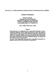
1.2 Industrial In-Plant Railroad Operation Large industrial plants in the chemical, automobile, and steel industry often stretch over entire quarters of cities. As in the case of steel works heavy freight such as molten iron has to be transported between widely spread production, storage, or shipping terminals. In order to maintain a timely around-the-clock production process it may be indicated to operate a private railroad system as a distinct legal entity, often a subsidiary. As such, an industrial in-plant railroad is subject to competition1 and has to be managed pursuant to economic aspects. Market deregulations in the railroad sector some years ago forced private railroads to offer a better transportation quality and to decrease charges. The efficient use—and desirably a reduction—of available resources became indispensable. Since the paper by C HARNES & M ILLER (1956), apparently no attention in the operations research literature has been drawn on this kind of railroads. Reason enough, to shed some light on the involved combinatorial problems. The remainder of this section is entirely devoted to a better understanding of the every-day operation and the surrounding decision making processes of an industrial in-plant railroad. Although the principles are generic, a steel mill serves as a good example for our exposition. Manufacturing of steel products such as chrome plated sheet is a multistage process. Melting iron, slab casting, cold reducing, or hot-dip galvanizing happens not only at different stages of the production process but also at different sites of the steel mill. From a railroad point of view these different sites or terminals are usually referred to as customers which are dichotomized according to their principal treatment of freight cars: Loading terminals request for empty freight cars suited for holding a specified intermediate, finished, or by-product, and unloading terminals order a certain quantity of raw materials or half-finished goods. The production plants of large industries may comprise several hundreds of such terminals, whose proper interaction has to be guaranteed by a customer oriented freight car switching . To this end, some industrial railroads run more than 100 switching engines , c.f. Figure 1.1 on the following page, to handle the flow of up to 6000 freight cars as depicted in the detail of a track layout in Figure 1.2 on page 5.

1.2.1 Hierarchy and Dependence of Planning Processes Apart from being impracticable, at least these days, decision making in complex planning processes is not carried out in a monolithic fashion, neither by human planners nor by computer 1 Competition in this context of course does not offer exchanging one railroad for another, but still, the management is exchangeable. And it is worth knowing that even the transport of molten iron by truck is possible today.

4

ENGINE SCHEDULING

Figure 1.1: A switching engine of Eisenbahn und H a¨ fen GmbH, Duisburg, Germany, transports molten iron at the steel works of Thyssen Krupp AG. These diesel or electric engines usually differ in their technical equipment, especially with respect to tractive effort, coupler, compressed air system, and radio control. Engineers have different skills and experience. Some need driving admissions for certain areas, particularly when driving on public tracks.

tools. In the simplest case, we have a sequence of decisions, often with feedback between single stages. Although from an optimization standpoint the hierarchical, or decomposition, approach wastes some optimization potential it usually reflects historically grown structures. For a fresh ¨ ¨ thinking on integrative perspectives see B ORND ORFER & L OBEL (1999). Figure 1.3 on page 6 gives an overview of the planning stages to be discussed next. As customary, we distinguish strategic, tactical, and operational issues according to the length of the respective planning horizon and the temporal impact and relevance of the decision. In brief, the three notions refer to planning in the long, mid, and short term, in that order. The Customer’s Planning

As Figure 1.3 suggests, the quantified customer’s demand for transportation provides the raw data for all decision making in in-plant railroad operation. Every movement of freight cars refers,

Figure 1.2: Inbound empty freight cars and raw materials, and outbound finished products and excess empty cars are interchanged with main line railroads like Deutsche Bahn Cargo in Germany, usually subject to a train schedule. Cars of inbound trains have to be decoupled and distributed according to their destination terminals. The moment when a car enters the in-plant track network is likely to differ considerably from the moment the customer is ready to process this car. The same is true for the reverse direction: Outbound rail cars from different customers but with a common shipping destination are intermediately kept on dedicated tracks before they leave the in-plant network at a later point in time. The problematic becomes especially obvious when cars are switched between loading and unloading terminals, or vice versa: It happens that freight cars which have to leave a loading terminal for some reasons are destined for a particular unloading terminal that is not yet ready to handle the cars. Analogously, yet unprocessed loaded cars at a certain unloading terminal may be needed elsewhere at a loading terminal. Although the overall production process of the steel works is coordinated, each customer is in a sense autarkic and has its own peculiarities.

1.2. INDUSTRIAL IN-PLANT RAILROAD OPERATION 5

6

ENGINE SCHEDULING

production planning

ope

ratio

nal

engine rostering crew rostering

engine scheduling car management

tact

ical

transportation requests Figure 1.3: Hierarchy of operational and tactical planning processes. The customer’s production planning, and request for transportation—represented by the circle—has direct impact on all actions of an industrial railroad—inside the circle.

directly or indirectly, to a particular customer. This is a significant contrast to public passenger transport systems being operated practically independently of individual demands. All the more important it is to strive for customer satisfaction by means of offering a high transportation quality, including e.g., timeliness. To set one spectacular example, an interruption of the blast furnace operation of a steel mill in consequence of an engine’s delay may cause major financial damage, for which the railroad company may be liable.

According to their supply contracts the customers devise a production schedule that determines the manufacturing program of each particular product. About a month ahead, this production scheduling is completed and serves as a mid term input for the railroad operation planning. This information is important inasmuch it constitutes an estimation of the expected quality and quantity of work, i.e., transportation, for particular working shifts. Production Planning

Whenever an unloading terminal runs out of raw materials or when the capacity of cars at a loading terminal is almost exhausted this terminal requests for service, which

Customer Requests

1.2. INDUSTRIAL IN-PLANT RAILROAD OPERATION

7

usually means exchanging the present cars for new ones. Apart from emergencies or unpredicted incidents no demand for transportation arises suddenly. However, there are customers who tend to issue their requests very late, even too late. Some of them request for immediate transportation although it is not operationally urgent. In such a case, the dispatcher is responsible for judging the priority of the respective request. As already mentioned, the customer information provided for each request usually specifies goods or cars in a certain quantity of a certain type only. Often only the purpose of the requested cars, say loading slag at the blast furnace, is transmitted and it remains up to the dispatcher to choose appropriate material, viz. cars and engines, to fulfil the request. Many tasks are obvious or regularly recurrent. They are taken into account by the dispatcher without explicit interaction with the customer, who expects this automatic generation of requests as part of the railroad’s service. We describe the proceeding of the dispatcher in more detail below. In-Plant Railroad Management Tasks

Long term decisions at industrial in-plant railroads involve purchasing or discarding engines and freight cars and re-designing the railroad track network. Although the network usually is historically grown it changes according to the changes and needs of the industrial plant it is located at. Nevertheless, for the rather short planning horizon we deal with in this thesis we may assume the infrastructure as well as the rolling stock and the operating personnel be fixed. Of course, deviations from the regular daily operation—like temporally closed tracks—may occur due to the realization of strategic measures and have to be considered in tactical and operational planning tasks. On the other hand, it is believed that there is an influence upward the planning hierarchy, viz. that an efficient planning at the tactical and operational level may result in cutting back the engaged resources and infrastructure in the long run, thus saving costs of the tied capital. Strategic Planning Issues

The railroad’s tactical planning process starts with the creation of a detailed engine roster for the next month. Based on the experience from previous months a standard roster is modified according to the peculiarities of the current planning period. The customer’s precursory production schedule helps to forecasting the demand of engines of certain types for every working shift of the planning period. Note, that from now on the engines’ places of employment are known. If necessary, engines are scheduled for regular maintenance at this stage. Engine Rostering

Crew Rostering Once the engine rostering is completed engineers and accompanying personnel have to be assigned to each rostered engine. The size of the crew—in rare cases up to four members—depends on the type of the engine and on the work it is supposed to do. The personnel must be qualified and permitted to operate the respective engine. When it is necessary to travel along public tracks outside the industrial plant the engineer needs a valid permission for doing so. It is not only advantageous that the engineers be familiar with the area where the respective engine will be operated but also it may be mandatory to have certain qualifications or specific

8

ENGINE SCHEDULING

knowledge when serving certain customers. Furthermore, collective agreements may regulate spare time claims, prescribed sequences of working shifts may have to be obeyed, and overtime hours are to be assigned fairly. Particularly in Germany, these regulations are hard constraints. Since the customers do not request for particular cars but for a certain transportation capacity or a specified input material the actual assignment of cars to requests is up to the dispatcher. This management of freight cars essentially hinges on the fact that only a small portion of the cars is actually owned by the railroad company. The majority of cars is rent from other railroads. Of course, cars are not identical and, especially in steel works, there are very special types of cars suited for a single purpose only. For all customer requests there usually is a certain type of car that fits best. However, it is often possible to replace certain types by others. From the customer’s production schedule it is roughly known which amount of which type of car will be needed in particular working shifts. Although this information is already given at the tactical level, it is hardly possible for manual dispatching to anticipate the exact stock of cars at the operational level. In case neither the required quantity of the best fitting type nor one of the replacing types is available additional cars have to be rent. Since paying the cars is on an hourly basis the dispatcher tries to return the cars as soon as possible, which in turn influences his or her assignment of cars. This is only one of the conceivable scenarios. Freight Car Management

Even having the required empty and loaded cars at hand does not imply that subsequent switching and transportation is uniquely predetermined. There may be several options to provide a customer with the requested cars, involving more or less switching and thus shorter or longer provision times. There is a tradeoff between expensive car rental and time consuming switching in order to make cars available. The goal is to minimize both the paid rent and the dead heading of cars while guaranteeing service without type mismatches. This problem is of a distinct combinatorial nature and deserves research investigations in its own right. However, this is beyond the scope of this thesis and will not be covered here in more detail.

1.3 Engine Scheduling and Transportation Requests We assume the aforementioned planning tasks completed, i.e., engines and crews are rostered, and appropriate cars are available and dispatched. Since the final stage of engine scheduling by nature depends on the incoming requests, both issues are discussed simultaneously. The customer’s demand for transportation arrives sequentially at the dispatcher’s working place by phone, fax, or radio transmission. These requests are gathered in a pool, ordered by non-decreasing due date which may range from a few minutes to several days ahead. Although this setting is inherently dynamic, it is legitimate to assume that for a planning period of, say, two hours our knowledge of future requests is (or can be made) sufficiently certain. Hitherto, we were considering customer requests like the demand for exchanging loaded freight cars for empty ones at a loading terminal. One such request may induce several sub-tasks like switching and coupling in order to make up a train of empty cars, hauling this train to a load-

1.3. ENGINE SCHEDULING AND TRANSPORTATION REQUESTS

9

ing terminal, weighing the fetched loaded cars, and switching them to their next destination. An experienced dispatcher immediately identifies all necessary sub-tasks, in the sequel referred to as transportation requests . Actually, the notion of transportation is slightly misleading because we will subsume also tasks that do not involve the movement of cars. More precisely, we have four categories that cover the whole range of our understanding of transportation requests: ➀ In-plant transportation This type of request is the standard operation and refers literally to transportation from an origin track to a destination track. Since often coupling and decoupling, checking the compressed air system, or discharging of cars is required at both tracks, the total duration of the request is longer than just the period of transport. ➁ Periodically scheduled trains All traffic interchange with main line railroads is bound to a train schedule. Possibly necessary preparatory work has to be completed when a train is due. Obviously, all requests in this category are completely known even weeks ahead. ➂ Local operation A terminal may require an engine to dwell for a certain while. For example during blast furnace tapping it is specified by safety regulations that an engine simply stands by in reach. Also, making up a train for a certain customer or a certain outbound direction may involve heavy, sometimes very time consuming, coupling, decoupling, and switching of cars. These are situations, when an engine stays at the same location, often at the same track. ➃ Exceptional and supplementary tasks So far we assumed an engine to be productive all the time. Actually, this does not properly reflect reality. Engineers have to have a break within a prescribed time interval of their working shift. Engines may not be available due to scheduled or unexpected maintenance and repair. The same applies for fueling an engine. Shift changeovers are only possible at dedicated locations and generally prevent engines from serving customers at the same time. Apart from rare exceptions all requests in this category are known at least one working shift in advance. The consensus of all these tasks is that the performing engine is allocated for an approximately known period of time; including preparatory work at the origin track and completing operations at the destination track. Such service may only be allowed during specified time windows , i.e., we have an earliest admissible commencement and a latest allowed completion of work. Such restrictions are determined e.g., by train schedules, berth periods of container ships, and deadlines for loading or unloading. Trains are weighed for the reason of cost accounting. Thus, the gross weight of the load is known, at least roughly. Comparing a request’s requirements with respect to technical equipment of the engine and skills of the personnel against the engines and engineers currently in duty immediately yields for each request the set of possible, or admissible, engines. At least theoretically, all engines may be admissible for particular requests. However, ordinarily, this set is constrained—for example non-availability of a catenary at a terminal requires a diesel engine, discharging of cars may require the appropriate air compression system, or fueling an engine restricts the set to precisely this engine. This list may be arbitrarily enlarged, but in either case checking admissibility is not

10

ENGINE SCHEDULING

difficult to implement, for instance by means of a binary vector representation of required and available items, respectively, for each combination of requests and engines. Based on the practical setting we will now start to elaborate a mathematical representation in order to work properly with the notion of transportation requests. We are mainly interested in a consistent treatment of all occurring cases. The attributes summarized in Table 1.1 suffice to capture all conceivable requests in the listed four categories. Given for a fixed planning horizon a set of requests2 and a set of engines, let us reproduce the above information in an arc weighted directed graph3 , c.f. Figure 1.4 on the next page. We will refer to as the request graph for a given instance. The node set comprises all tracks with relevance for engines or requests. More precisely,

r r e e ! r

"#

e

where e , e are virtual tracks associated with the end of service of the respective engine. Note, that instead of physical locations which may be identical, nodes represent logical tracks are joined by an arc i j if and only if sequentially which are all distinct. Two nodes i j visiting the logical tracks i and j, in that order, is operationally plausible for some engine. Briefly, service will not start with a destination track, will not end at an origin track, and the origindestination sequence of a request must not be reversed. To be exact,

$ "%

"&

' e r) r r * r e e e+, . r r r r r r r r !/ ( - 1 2

e

r

1 2

1 2

1 2

(1.1)

r1 r2

Although every sensible sequence of duties for an engine corresponds to a directed simple, i.e., node disjoint path in , the converse needs not be true. This issue will be dealt with rigorously in Section 1.5. Referring to the load to be picked up or delivered at a particular location r or r for r we will also use the notation r 0. Finally, let r . Note, that r r us shortly demonstrate the modeling flexibility of the attributes listed in Table 1.1. The request data, except for the tracks, are of course all optional and assume by default their respective largest degree of freedom, e.g., time windows are set to the entire planning horizon. If the particular location is of no importance, as for breaks, our logical tracks can be made close to everywhere by setting all respective ti j to zero. An engine e may exclusively be reserved for stand-by or similar activity by setting Le 0. Also, time windows can be used to reflect high or low priorities. In fact, our mathematical understanding of a transportation request goes beyond what is customary used in practice.

"0

1 2 4351 6 71

1 6&8

The average velocity of an engine depends on whether cars are attached or not. Steep grades or small radii of bends may prevent a loaded, and only a loaded, engine from traversing

Remark.

2 Referring

9 : ;=

to transportation requests, from now on we will mostly use the short form request. graphs in this thesis are simple, i.e., there exist no loops i i , and no parallel arcs. Denoting arcs we will interchangeably use, both, i j and i j . 3 All

9 : ;@

1.3. ENGINE SCHEDULING AND TRANSPORTATION REQUESTS

planning horizon network data, i j

"A

engine data, e

"B

request data, r

"0

ti j ci j Le e te te

C 2 E2 D r , r sC 2 , s 6 C tt 26 tt 2F6GDD 1 r

r

r

r

r

r r

r

11

set of transportation requests set of available switching engines time required for traversing arc i j cost incurred when traversing arc i j tractive effort (i.e., capacity) of engine e (logical) track where engine e starts its service time window during which e becomes available set of admissible engines for request r (logical) origin and destination tracks service time at origin and destination tracks start-of-service time window for origin track start-of-service time window for destination track size of the load to be transported

Table 1.1: Summary of input data for an engine scheduling instance

e

r

r

Figure 1.4: Schematic structure of the request graph

e

12

ENGINE SCHEDULING

certain tracks. Other tracks may not be usable for certain types of engines due to technical constraints. However, we will not distinguish notationally between individual graphs and associated travel time and cost matrices, and assume that always the appropriate data, if available, is used. Of course, this is no problem in a computer implementation. Current Manual Dispatching is Based on Passive Information Systems

To put it simple, engine scheduling is to allocate engines to transportation requests. Within noteworthy operational tolerances this fixes a sequence of requests with their associated service times for each engine in duty. In order to assure customer satisfaction, a punctual service must be enabled by the respective assignment for each engine. The tractive effort of an engine must never be exceeded. The scheduling process is decentralized such that each dispatcher is responsible for no more than ten or twelve engines, often significantly less. Still, a human judgment of dependencies between different decisions of such complexity is necessarily local and incomplete. Although the dispatcher creates the schedules, their realization is beyond his or her control. The productivity of crews varies considerably as was already stated by C HARNES & M ILLER (1956). The same operation will require different execution times for different crews, sometimes deviating by more than a factor of two. Moreover, weather conditions greatly influence the duration of transportation requests. In winter, cars have to stay in defrost facilities prior to being unloaded. Thus, large portions of the input data does depend on human experience and, at least these days, rest upon estimations. We will consider all human decisions regarding the input data as irrevocable. Present computer aid is essentially limited to providing information on the status quo, e.g., a graphical display of the scaled track layout, the location of cars and engines, and relevant data about outstanding transportation requests, c.f. Figure 1.5 on the facing page. In a sense, a key functionality of these systems is to track the dispatcher’s past decisions. We would like to refer to such kind of decision support as passive.

1.4 Computer Aided Scheduling One might expect that in a workaday industrial operation an experienced dispatcher will anticipate many of the requests, and schedule the engines accordingly. While in normal operation this is actually true, under peak workload looking ahead is practically impossible. Then, requests are served on a first-come first-serve basis, or, more realistically, in a manner depictedly termed loudest-shout first-serve. For this reason, industrial in-plant railroads typically operate more engines than are actually needed in standard situations. For all railroads utilizing more than eight engines there is a considerable overhead of up to one fifth of all engines. The question arose how to achieve a more regular and steady-going operation in order to mitigate these inefficient and resource consuming peaks. This motivated the incorporation of a computer aided scheduling tool into existing systems, which is able to offer an active decision

1.4. COMPUTER AIDED SCHEDULING

13

Figure 1.5: Screen shot of the information and dispatching software CP-BIS by CSC Ploenzke

support and relief for the dispatcher. Such a tool should submit scheduling suggestions that take into account all information available to the system. This enables one not only to individually respect the needs of particular customers but also to pursue operational, i.e., quantifiable goals. Note, that at present a schedule is of sufficient quality when it is feasible. A global view on the ¨ production process much better allows for exploiting the rationalization potential. B ORND ORFER ¨ & L OBEL (1999) detail further advantages compared to conventional planning.

Operational Goals

Although a reduction of the number of engines is aspired in the long term this will be achieved only mediately by improving the resource usage at the operational and tactical level. Conceivable measures include decreasing the total mileage traveled by the engines. In view of the unavoidable transport induced by transportation requests it could be better to increase productivity by reducing dead heading and waiting times instead.

14

ENGINE SCHEDULING

Ideally, the respective gains should be exploited to the largest possible extent. In other words, with respect to a given operational goal, the desired computer aided scheduling tool should produce an optimal scheduling suggestion. It is one of the aims of our research to provide the necessary mathematical technology underlying such a tool, i.e., models, algorithms, and implementation considerations.

1.5 Pickup and Delivery Problems Time constrained routing and scheduling problems received much attention in the operations research literature, see D ESROSIERS , D UMAS , S OLOMON & S OUMIS (1995) for a recent survey, and D ESAULNIERS , D ESROSIERS , I OACHIM , S OLOMON , S OUMIS & V ILLENEUVE (1998) for a unified framework. Generically, when weights are to be transported in time from origins to destinations by a fleet of capacitated vehicles we speak of the multiple-vehicle pickup and delivery problem with time windows (m-PDPTW). For its relevance to our practical situation we will now access some characteristics in more detail.

K/K/L/K NMO "B

HIJ

Definition 1.1 (Pickup and Delivery Path) as defined above. Let R e i1 i2 iν e an ordered set representing Let a directed simple path in for an arbitrary but fixed e . R is called pickup and delivery path if and only if the following conditions hold.

r PM R or r r Q R 0,/ for all r "0 (ii) If i r and i r for an r "R then ν S ν (iii) ∑ . 1 8 L , for all ν 8 ν (iv) Let T max t 2T t 2 t T s and T max T T t 2 t T s 2 2 Then T 8 t for 1 8 k 8 ν (v) If r " R then e "U (i) Either r ν1

ν2

ν1 k 1 k

e

1

2

1

e

k

1

e i1

i1

i1

k 1

ik

k

ik ik

1

ik

1

ik

1

, for 1

8 kS

ν.

r

The conditions (i) through (v) will be called pairing , precedence, capacity , time window , and admissibility constraints, in that order. Condition (iv) respects that arrival at a location is allowed

before the corresponding time window opens, but this incurs a waiting time. A feasible solution to the m-PDPTW is a set Re e of (node sets of) pickup and delivery paths such that

V R ! e

e

(1.2)

i.e., the paths partition the set of nodes. Actually, they induce a partition of the set of requests as well. Note, that Re e e conforms to Definition 1.1, which is required to account for the possibility of not using engine e .

"W

1.5. PICKUP AND DELIVERY PROBLEMS

15

Recent Research Topics

S OL (1994) and S AVELSBERGH & S OL (1995) comprehensively review several characteristics and the relevant approximative and exact solution approaches to the pickup and delivery problem in its variants. In particular, they develop the most general presentation of the m-PDPTW to date, which allows a multitude of pickup points and of delivery points, respectively, for each transportation request. D ESAULNIERS , D ESROSIERS , E RDMANN , S OLOMON & S OUMIS (2000) additionally provide a catalog of practical applications. Benefitting from these survey papers, we will only comment on some of the most recent literature. Details on earlier work will be deployed throughout the text whenever relevant to the context. O ERTEL (1997) considers the m-PDPTW with transshipment allowed at predefined locations at linear cost. To this end, transportation requests are split in two (at least), thus artificially enlarging the problem size. The additional problem arises that, at transshipment locations, vehicles can only pick up a load already delivered by another vehicle. This may even lead to deadlock situations. O ERTEL describes criteria to prevent such situations and proposes adapted TSP heuristics to create solutions for instances of up to 100 customers. The dial-a-ride problem (DARP) is an important special case of the m-PDPTW, in which transportation requests correspond to passengers. It arises in the transportation for the handicapped and the elderly. Thus, additional constraints are present e.g., the need for loading wheel chairs. An approximate solution to DARPs is indicated because of the large size of practical problem instances (up to 6000 requests). A common heuristic approach to vehicle routing problems is cluster-first route-second, in which the assignment of requests to vehicles, and the determination of the sequence of visited requests for each vehicle is not performed simultaneously but in two subsequent phases. Two mini-clustering approaches were recently suggested, both of which group small numbers of passengers into clusters according to heuristic criteria. This step is formulated as a set partitioning problem, c.f. Section 2.1.3. I OACHIM , D ESROSIERS , D UMAS , S OLOMON & V ILLENEUVE (1995) then solve an asymmetric m-TSPTW on the set of clusters, ¨ ¨ ¨ whereas B ORND ORFER , G R OTSCHEL , K LOSTERMEIER & K UTTNER (1999) allow vehicles to wait before starting the next cluster. Again, the routing phase is modeled as a set partitioning problem in both papers. RULAND & RODIN (1997) investigate the polyhedral structure of the polytope associated to the convex hull of incidence vectors of 1-PDP paths. They derive some classes of valid inequalities to be incorporated in a branch-and-cut algorithm. Their code is able to solve instances of up to 15 customers in reasonable time. From this the authors conclude that the strength of the identified valid inequalities is insufficient. To the best of our knowledge, this is the only study in polyhedral combinatorics which has been proposed so far; particularly the statement of facet defining valid inequalities is still outstanding. As for many combinatorial optimizations problems, very few is known about the so-called online situation of pickup and delivery problems, in which the knowledge about future requests is incomplete. In practice, one is often badly advised with the acknowledged theoretical concept of competitive analysis for evaluating the performance of online algorithms. The lack of a satis-

16

ENGINE SCHEDULING

factory theory, in particular for the PDPTW, will certainly be a research incentive for the years to come. A SCHEUER , K RUMKE & R AMBAU (2000) made first moves into this direction with their investigation of the online DARP. With respect to competitiveness they propose a best possible online strategy, called smartstart, to serve transportation requests without time windows in a metric space. Their objective is to minimize the makespan, i.e., the completion time of the last vehicle. H AUPTMEIER , K RUMKE & R AMBAU (1999) furthermore compare intuitive scheduling strategies under the assumption of an infinite planning horizon. The classical nearest neighbor heuristic for the TSP relies on a measure of proximity of two requests. As some authors point out, such a measure is not that obvious in the PDPTW situation. I OACHIM , D ESROSIERS , D UMAS , S OLOMON & V ILLENEUVE (1995) introduce the concept of neighboring requests in the E UCLIDEAN plane. Two requests are said to be neighbors if their time windows overlap, the respective locations are “close” to each other, the travel directions do not exceed a specified angle, and savings in travel time can be realized by jointly serving both requests. Last, but not least, attempts have been made to unify various vehicle routing problems, revealing the PDPTW as a special case of a general framework of considerable complexity. For instance, D ESAULNIERS , D ESROSIERS , I OACHIM , S OLOMON , S OUMIS & V ILLENEUVE (1998) propose a non-linear mixed integer program which also encompasses the possible linkage between different vehicle routes, e.g., to represent precedence relations between requests. For computational experiments see I OACHIM , D ESROSIERS , S OUMIS & B E´ LANGER (1999). Objective Functions

A multitude of objectives has been proposed, see S AVELSBERGH & S OL (1995) for an overview. Minimization of the fleet size is common for DARP situations in which vehicles are rent on a day-by-day basis. As mentioned above, dead heading and waiting times are undesired for our practical problem. Therefore, one may explicitly minimize these two quantities, or we may chose as objective the minimization of the total time needed for all the vehicles to execute their paths, also known as route duration. Both objectives possess certain practical disadvantages, c.f. Figure 1.6 on the next page. However, with a rolling planning horizon the former may prove more appropriate. In many vehicle routing problems there exists a hierarchy of goals, e.g., primarily minimize the fleet size, and secondly minimize a mileage or travel time dependent goal. Practitioners from in-plant railroads were sceptical about primarily reducing the number of engaged engines. This might change when suggested schedules prove that on average a number of engines is not needed.

1.6 Concatenation: A Framework for Engine Scheduling The m-PDPTW is a flexible model capable to cover such various applications as door-to-door transportation systems as well as managing the parcel collection and distribution of a parcel

1.6. CONCATENATION: A FRAMEWORK FOR ENGINE SCHEDULING

i

e

r

e

17

i

j

j

e

Figure 1.6: Pathology of objective functions. Consider minimizing the sum of route durations on the left. Request rlate arg maxr t r determines the route duration of the engine which serves it. Considerable dead heading may occur on this engine before r last is served; schedules may be bad with respect to total travel distances. When dead heading time is explicitly minimized, c.f. the picture on the right, a related effect may occur. Instead of serving the depicted requests i and j consecutively, the two requests could be served as indicated by the dashed line. In effect, the engine runs less empty, but the mileage increases. At the worst, some request r is picked up, then serving other requests is for free (the engine is not empty all the time), and finally r is delivered.

6

service. While the generic model is definitively suitable for our practical situation, our additional knowledge about the problem structure is not adequately exploited. In a sense, the m-PDPTW is too general, in that it offers a flexibility we do not encounter in practice. Railroads and Pickup and Delivery Problems

Railroad traffic imposes certain particularities on the m-PDPTW. At first, vehicle capacity is very restrictive. For instance, a switching engine is usually not powerful enough to haul more than two or three of the special type rail cars which hold molten iron, c.f. Figure 1.1 on page 4. Secondly, the loading and unloading operation itself is distinct. As a consequence of moving along railroad tracks the most reasonable loading scheme is last-in first-out. Clearly, deviation from this scheme incurs extra work in form of time consuming switching operations. Thus, in general the sequence of served requests will influence the individual processing times, which requires a warily choice of simultaneously served requests. This motivates the approach of restricting pickup and delivery paths to be built of a preselection of sensible loading/unloading sequences, leading us to the notion of precast request patterns.

X Z Y [\^] _` a b _` ` f k Y [ l@m P n k Y [\

Definition 1.2 (Pattern, Family of Patterns) An ordered subset P r r of nodes is called pattern if and only if there exists an r e such that the node sequence given by e P e is a pickup and delivery path. A family of with patterns is a set of patterns such that there exists a

ced

a

fhgiXjf ] r_ ` r a bo In order to access the set of requests visited by a pattern P cUf we use the notation requests p P q : n ] r c0r s r _ ` r a c P b!o P

r

(1.3)

18

ENGINE SCHEDULING

] _àb

c&r

_

The simplest non-empty pattern, which we will call full truckload for historical reasons, is r r for a given r , i.e., immediately delivering the load picked up in r . Note, that each node is allowed to be contained in different patterns of a family. Observe, that our definition of a pattern only predetermines the precedence or sequence of contained nodes, not the respective visiting times, i.e., the schedule itself. However, by Definition 1.1, for each pattern there exists a schedule which is feasible with respect to time window constraints. Moreover, in the modeling phase we will use the following.

f

Lemma 1.3 (Properties of Pattern Families) A family of patterns has the following properties. (i) For each r

c0r

(ii) ∑ p

0 for all P

[ u n P p

(iii) If for any r (iv)

there exists a P

c0r

cWf

we have r

_n

cBf

i p1

] _ ` r a btX

with r

P

c ] i `KoKoKov` i bwn P Uc f 1

ν

then r

syfAs is finite but not necessarily polynomially bounded in s r s

an

i p2

c

P and p1

x

p2

z

Proof. Follows immediately from Definitions 1.1 and 1.2.

{|n p }I`~q

Clearly, the family of largest possible cardinality is the collection of all pickup and delivery paths in . It is more interesting to restrict attention to a (small) subset of (simple) patterns, and use them to form more complicated paths. In the following we will do precisely this, exploiting the fact that a vehicle is empty after having visited all locations of a pattern.

f

f

n ] _ ` òKoKo` ` a b be a pickup and delivery path. R is n KK p n ν exist such that ] i `KoKoov` i b ` ] i _ ` oKoKo` i b`KooKo` ] i _ òKovo` i btcBf o

Definition 1.4 ( -Concatenation) Let be a family of patterns, and let R e i1 iν e called a -concatenation if and only if indices 1 p 0

f

p0

p1

p1 1

p2

pk

k

1

1

pk

We will also refer to the act of constructing such paths as pattern concatenation.

f

Remark. Although this definition allows multiple visits to requests we will assume throughout this thesis that -concatenations be request disjoint unless otherwise stated. A concatenation with repetition of requests may illegitimately incur less waiting times or dead heading, and thus amplify the effects depicted in Figure 1.6. We will see later on that request disjointness has substantial implications on algorithmic design.

f

Figuratively speaking, by preselecting a family of patterns we constrain each customer’s context in admissible pickup and delivery paths. Note, that it is not known beforehand whether a given P will be incorporated in any concatenation. Again, the empty concatenation e e for an e conforms to this definition. We will particularly focus on concatenations made of the following families.

cf cd

] _` ab


i i

_

i

a

j

_

i

_

_ _

j i j

a

a

j

a

i

19

a

Figure 1.7: Typical situations for full truckload, overlapping, and embedding requests

f

s r4s

Definition 1.5 (Regular Pattern Families) The set k of patterns which visit exactly k requests out of , and which are not concatenations i, i of patterns P k, is called k-regular pattern family , for k 1 .

cWf x

s r4s

n `KoKoLoK`s r4s

is a multiple of k. Nevertheless, we Note the technical particularity that (1.3) holds only if will consider unions of such regular pattern families which will always admit feasible concatek nations. From Lemma 1.3 (i) it is clear that each P 0/ contains the origin and destination node, respectively, of exactly k requests. According to officers of in-plant railroads involved in our research, only the very simplest patterns do occur in practice, namely

cUf n

fX k Y [\ ] i_ ` ia b k Y [\^ ] i_ ` j_ ` ia ` j a b ] i_ ` j_ ` j a ` ia btn!f f o i

1

i j

2

(1.4)

Reasons for this simplicity do not only emerge from the restriction to railroad tracks but also from the need for acceptable working conditions for the engineers. Figure 1.7 shows the structure of the three basic types of patterns which are called—besides the already known full truckload—overlapping and embedding , lending their names from the temporal relation of the involved requests. Actually, current manual dispatching constructs mostly full truckload patterns, and only a small fraction of patterns in 2 . Note, that the choice (1.4) of patterns is not equivalent to allowing at most two requests to be served simultaneously on one engine, since for example i j j k k i for i j k is not allowed. We will follow up some further matters related to -concatenations, which are not an issue here, in Chapter 6.

f n n Rc r

] _ ` _ ` af ` _ ` a ` a b Given a family f of patterns, Definition 1.2 ensures the existence of patterns which partition r . However, it is not guaranteed that there exists a partition which allows f -concatenations to

be constructed for all engines. For instance, time windows could be conflicting for patterns to be served on the same engine. Nonetheless, current (feasible) schedules suggest that the above choice of the pattern family (1.4) is reasonable and always allows a feasible solution. Capitalizing 1 2 , we are now able to on the above definitions, and abbreviating from now on 1 2 : state our problem in a very compact form.

f n f f

20

ENGINE SCHEDULING

d r f

Z Y [ ] b !n [}

Definition 1.6 (Engine Scheduling Problem) Given and , a feasible solution to the engine scheduling problem (ESP) is a set R e feasible 1 2 -concatenations such that their disjoint union visits all nodes, i.e., e Re

of .

e

The introduction of patterns allows for sequence dependent service and travel times (and cost). That is, we are able to account for the extent of work required at a particular location in dependence of the cars picked up previously. To simplify matters, we will not introduce a separate notation for individual arc weights. Again, this causes no difficulty in a computer implementation and we will assume that the appropriate data is used, if available.

Remark.

Figure 1.8: Structural appearance of a

Lemma 1.7 For any m in the strong sense.

f

1 2 -concatenation

1, minimizing the sum of route durations for m-ESP is

] sdUb s [ s r^} s

} f

cOd

-complete

f

1 2-

}^f Completeness in the strong sense follows from restriction to the m-TSP with time windows as follows. Split each city i of an m-TSPTW instance into ] i _ ` i a b , and assign to both nodes the same time window as city i has, and service times of zero. Let t n c n 0. Arcs entering (leaving) city i in the m-TSPTW enter i _ (leave i a ) in the m-ESP instance. The respective arc weights are preserved. Allow only f -concatenations for the m-ESP, e.g., by defining L n 1, e cWd , and u n 1, r c0r . Clearly, an optimal solution to this instance immediately gives rise to z an optimal solution to the corresponding m-TSPTW instance in polynomial time. Proof. Guessing a partition Re e of and checking whether each Re , e concatenation is polynomial in and . Hence, m-ESP is in .

i i

is a

i i

1

e

r

}^f

The proof can be adapted to other objective functions as well. In fact, S AVELSBERGH (1985) proves that even finding a feasible solution to the TSPTW is -complete in the strong sense. Therefore, by the same construction we have Lemma 1.8 For any m in the strong sense.

1, the problem of finding a feasible solution to m-ESP is

}^f

-complete

To the best of our knowledge, no research efforts have been undertaken in the direction of pickup and delivery paths of restricted combinatorial structure. This contrasts our experience that practically all computational experience reported on the PDPTW that we are aware of is drawn from problem instances allowing only a very special structure of paths. The interested reader


21

will verify for example in D UMAS (1985) and D UMAS , D ESROSIERS & S OUMIS (1991) that the ratio ρ

n

maxe minr

c ] ` b

[ L [\ u

e

(1.5)

r

rarely exceeds very small integers, say ρ 2 3 . This observation is valid both for artificial and real world instances. Fairly large is ρ 5 (S OL 1994), but also only ρ 1 is considered (D ESROSIERS , L APORTE , S AUV E´ , S OUMIS & TAILLEFER 1988). Heuristically, patterns of “large” cardinality, i.e., patterns in k , k ρ, could be forbidden. Moreover, the practical situation might explicitly enforce precisely this—which is true for our application.

f

n

All cited authors conclude from their computational investigations that computation times decrease for highly constrained instances in terms of vehicle capacity. In dial-a-ride systems temporal constraints imposed by the customers strongly restrict the total vehicle load at any point in time, and the capacity constraints are of secondary importance (D ESROCHERS , L ENSTRA , S AVELSBERGH & S OUMIS 1991). Moreover, large fleet sizes are assumed by most authors. With as many vehicles available as half the number of requests (S OL 1994), we cannot obtain “complex” paths in any solution, even if, say, only one third of the fleet size is actually used. Also, clustering approaches produce on average mini-clusters of size less than four (D ESROSIERS , D UMAS & S OUMIS 1987), or two or three, respectively (I OACHIM , D ESROSIERS , D UMAS , S OLOMON & V ILLENEUVE 1995). Thus, in consideration of practical needs, we feel a methodological exploitation of these facts is overdue. In fact, besides delivering a model and a solution approach to in-plant railroad engine scheduling, a first step is contributed by our research.

Distinguishing Properties of the Engine Scheduling Problem

In order to properly delimit the ESP definition we would like to describe some neighboring properties which do not hold. At first, the common notion of depot—i.e., a start and return point of each vehicle’s itinerary—is void because open paths are usually sought instead of closed cycles. It is important to point out that the intention of -concatenations is not a cluster-first route-second approach in which all constructed clusters are actually built into routes. Instead, always a strict subset of will be selected simultaneously to the construction of concatenations. Therefore, this approach is designed to be exact, provided is inherently given by the problem.

f

f

f

Another contrast to the two stage strategy of cluster-first route-second is that patterns do not ¨ fix the temporal relation of nodes, i.e., travel times within a pattern. For instance, B ORND ORFER , ¨ ¨ G R OTSCHEL , K LOSTERMEIER & K UTTNER (1999) force a vehicle not to wait within a cluster. Thus the total cluster duration is known in advance. This is reasonable in their DARP setting but would unduly constrain flexibility in our context. In particular, the ESP is not a fixed schedule problem altogether, i.e., node visiting times must be explicitly determined in a solution approach. This has known complicating consequences both on model building and algorithmic design.

22

ENGINE SCHEDULING

Change in Problem Character

We deem it important to emphasize a consequence of our development in this section. Although originally based on the PDPTW, the ESP profoundly differs from the latter in its problem character due to the introduction of -concatenations. Pairing, precedence, and capacity constraints, respectively, which are essentials of the PDPTW are explicitly controlled by the precursory choice of a pattern family. Instead, besides time window and admissibility constraints which are common to both problems, the ESP is governed by decisions on selecting patterns that appropriately partition the node set . On the one hand, this strongly suggests to focus the model design on this selection. On the other hand, it inhibits, at least it aggravates the use of simple node oriented construction methods like straight forward adaptations of shortest path algorithms.

f

}

Further Applications of Pattern Concatenation

Empirical motivation for drawing attention to special structures of pickup and delivery paths comes from (1.5). We conclude with an outline of practical problems to which pattern concatenation is related, and where it may be a reasonable potential modeling alternative or complement. The references given are often only a representative for the respective problem class. FAGERHOLT & C HRISTIANSEN (2000) consider seaborne transportation of various dry bulk cargos by a heterogenous fleet of ships in northern Europe. The problem structure is an m-PDPTW with a few loading ports and comparably more unloading ports. Each ship is equipped with a cargo hold which can be flexibly partitioned by means of variable bulkheads in order to lift different cargos simultaneously. The positioning of the bulkheads in one particular port may influence subsequent scheduling decisions, similar to the ESP where single schedule decisions have consequences for the amount of switching later on. Furthermore, the problem is well constrained in terms of compatibility between ship, port, and cargo particularities. Additional requirements concerning e.g., a safe trim of the load may be an issue. Also do coastlines impose restrictions on the sequence of ports to be visited. Consequently, the set of sensible loading/unloading patterns is severely constrained in its combinatorial complexity—a potential application area of pattern concatenation, possibly with an adapted definition of patterns, since ships need not necessarily become empty so often as our engines do. For the special case involving only one coastline we refer to Theorem 6.15 on page 149. Ship Scheduling

¨ Extraction of Logs in Forestry R ONNQVIST , W ESTERLUND & C ARLSSON (1998) report on an economically utmost important practical operative problem in Swedish highly mechanized forestry, viz. the extraction of roundwood from felling points to forestry roads in as short time as possible. Two types of vehicles are employed. Harvesters actually fell the trees and compile logs based on assortments which principally reflect the demand of the respective saw and pulp mills. These piles are collected by forwarders and moved to larger piles adjacent to forestry roads. Each forwarder starts its trip with empty driving to the first pile to pick up, and continues


23

loading logpiles until it is fully loaded. Then it returns to the appropriate pile (or piles) in order to get unloaded. Time windows are of no special importance. Several assortments can be loaded on a forwarder, however, only in predefined patterns. Figure 1.9 shows sectional drawings of different admissible such arrangements. Choosing one of the depicted patterns basically fixes the order in which piles are loaded and unloaded, e.g., because of risks the forwarder could tip over. It remains the decision which piles to actually load. However, for a given region this follows almost canonically from the way the harvest is done. With respect to our concept, pattern families could be devised for the sequence of loading each particular assortment in the respective regions, or even for each of the depicted arrangements of assortments. A

B

C A B

C D A B

B A

C B A

Figure 1.9: Arranging assortments of wood on a forwarder vehicle. The different letters indicate different assortments. Each assortment may be filled by loading more than one pile, when it is not too complicated, operationally. On average, five piles are loaded on one forwarding route.

In order to meet the strongly increasing volume in maritime container transport, the HHLA CTA GmbH, Hamburg, Germany, plans to operate an almost fully automated container terminal. Concerning seaside operations, container vessels are loaded/unloaded via double rail mounted gantry cranes, and container are transported by means of uniform automated guided vehicles, or AGVs, to/from the intermediate stowage areas. AGVs navigate via electronic marks in the ground, thus, focus is on assigning and scheduling the transports. Interestingly, an AGV may lift either one forty feet container or two twenty feet container simultaneously. Therefore, each trip corresponds to serving either a 1-regular or a 2-regular pattern. Punctuality is a crucial factor to this operation, and what is more, permanently new information about e.g., container destinations is made available to the scheduler. This problem can be seen as an online and real time variant of the ESP.

Scheduling of Automated Guided Vehicles

E RDMANN , N OLTE , N OLTEMEIER & S CHRADER (1999) simultaneously determine aircraft rotations and passenger routes for an airline in the charter business. Since each aircraft basically alternates between a home country and some vacation targets, daily schedules, i.e., the respective sequences of direct flights, are often simply structured. This extremely simplified problem exposure is not originally in the pickup and delivery context, but an example for numerous network design applications. The general problem consists of determining a minimum cost flow in a network which is not a priori given but simultaneously constructed. Design decisions usually may involve nodes and arcs. In addition, we may involve a possibly broadened definition of patterns. It must be stated clearly, that building a pattern P is not equivP A of the underlying graph G, where A denotes alent to simply aggregating a subgraph G Airline Schedule Generation

g np ` q

24

ENGINE SCHEDULING

the set of arcs induced by P in G. Aggregation would imply that if any arc in A is designed then this holds for all arcs in A, while in pattern concatenation arcs may appear in different patterns, and the implication is not valid. It is to be checked for the respective application whether a better exploited problem knowledge justifies the potential overhead involved by our approach.

CHAPTER

Selected Topics in Column Generation It was just very very very big, so big that it gave the impression of infinity far better than infinity itself. —D OUGLAS A DAMS , The Hitchhiker’s Guide to the Galaxy

Over four decades have passed since F ORD & F ULKERSON (1958) contemplated to deal only implicitly with the whole set of variables of a multicommodity flow model. DANTZIG & W OLFE (1960) pioneered this fundamental idea in a general setting, developing a strategy to columnwise extend a linear program as and when needed in the solution process. In their ground breaking papers on the cutting stock problem, G ILMORE & G OMORY (1961, 1963) were the first to make actual use of the technique, soon to follow by e.g., A PPELGREN (1969). Today, more than ever, column generation is a prominent—and sometimes the solely applicable—method to cope with linear programs1 having a colossal number of variables. Although the basic concept stayed the same, its environment continuously developed throughout the years. The embedding of column generation techniques within a linear programming based branch-and-bound framework paved the way for the exact solution of large-scale integer programs. Starting with the work of D ESROSIERS , S OUMIS & D ESROCHERS (1984) on routing problems with time windows, numerous practical applications were to follow. Huge programs to be solved only became huger, most drastically in the 1990s. Here, we will meet some challenges of tomorrow’s hugest problems. It is the aim of this chapter to provide a synopsis of the methodology according the author’s personal preferences. It is partly close to, but not primarily intended for an inclusive literature 1 Although

the column generation context is much broader, we restrict ourselves to linear programming.

25

26

SELECTED TOPICS IN COLUMN GENERATION

survey. In our presentation, there is a bias towards incorporating mainly recent material that has ´ not found its way into textbooks, yet. Each of C HV ATAL (1983), M INOUX (1986), NAZARETH (1987), and W OLSEY (1998), devote a chapter to the basics. L ASDON (1970) is an amazingly valuable source of information on large-scale optimization. The surveys by BARNHART, J OHN SON , N EMHAUSER , S AVELSBERGH & VANCE (1998) and D ESROSIERS , D UMAS , S OLOMON & S OUMIS (1995), and the thesis of VANDERBECK (1994) are truly insightful. D ESAULNIERS , D ESROSIERS & S OLOMON (1999) is an indispensable computational reference. Besides the above publications, there exists a column generation jigsaw puzzle scattered all over the vast literature. More than one half of this thesis’ bibliography entries are referred to in this chapter—compiling 117 citations in total. As of this writing, some new fascinating ideas are available as technical reports only. A good deal of the findings related to our “selected topics” are nowhere stated as provable theorems, but hidden between the lines as observations and remarks. Whenever possible we try to merge kindred contributions, preferably making the outcome an explanation for empirical phenomena. Particular applications or even single problem instances gave the impetus for some interesting developments. Sometimes authors refer to intuition, and indeed, so do we occasionally. It is not easy, if not impossible, to discuss the components of a column generation scheme separately or independently. More explicitly, our “selected topics” are strongly interconnected. An introductory methodology outline will help us to get to grips with the dependencies. Nevertheless, some concepts and notions will be casually used before their proper introduction. In this chapter, we are mainly concerned with the linear programming setting. However, throughout the whole chapter it is instructive to keep in mind that our ultimate aim usually is to solve an integer program, although the presentation of the procedure for doing so, branch-and-price, is deferred to the very end. As linear programming techniques are indispensably located at the heart of integer programming solution approaches, the classical methodology of linear programming column generation is the most important building block of integer programming column generation. Arguably, there are no new results in this chapter. Still, we are not aware of a comparable accumulation of various sources, enabling us to find better ways to relate things. Hopefully, the chapter will successfully do this, conveying a clear understanding of fundamental and some more advanced ideas in column generation. They are the key to the success of the approach developed in this thesis.

2.1 Decomposition and Extensive Reformulation Integer programs and their associated linear relaxations encountered in applications almost always exhibit a large deal of structure. Constraint matrices are typically very sparse, having non zero elements in the order of magnitude of one percent, or less. This well known phenomenon is due to the fact that activities associated with variables are subject to only a few of the conditions represented by the constraints, respectively. On top of that, there may exist a hierarchical, geographical or logical segmentation of the underlying problem, which is reflected in the model formulation. Thus, it is likely that the non zeros are grouped in such a way that independent sub-

2.1. DECOMPOSITION AND EXTENSIVE REFORMULATION

27

systems of variables and constraints result, possibly linked by a distinct set of constraints and/or variables. Figure 2.1 shows schematically the distribution of non zeros for different angular block diagonal matrices, occurring in practice most frequently (M INOUX 1986).

Figure 2.1: Block diagonal matrix structure, (a) with linking constraints, (b) with linking variables, and (c) with linking constraints and variables. Only the shaded regions may contain nonzero elements.

The general idea behind the decomposition paradigm is to treat the linking structure at a superior, coordinating, algorithmic level and to independently address the subsystem(s) at an subordinated level, exploiting its structure. Here, we are concerned with linking constraints only. By the way the aforementioned coordination is handled, the resulting approaches are usually called price directive. See e.g., the techniques of B ENDERS (1962) and VAN ROY (1983), respectively, for the treatment of the other two cases. Consider the following general problem

pq

c% c

min c x subject to Ax x

X _

c

b S

`

(CF)

m n, b m , and S n . The cost function c : n where A is not required to be linear. For the purpose of this chapter we will refer to (CF) as the original or compact formulation. The seeming distinction of different kinds of constraints allows us to uniformly treat different variants of this problem. It should be mentioned that such a decomposition can be applied to any (linear) program, since constraints and variables can always be partitioned, albeit artificially, into subsets. We focus in this section on strategies that exploit structural properties of the constraint matrices and allow for a reformulation of our compact model which is easier to solve or which offers other advantages. Later on we will show how to actually solve the resulting reformulations by column generation, a methodology inseparably connected to the decomposition approach. We will especially take into consideration the benefit of the discussed techniques for the solution of large integer programs.

Before we start, let us make some general remarks. Models with a large number of variables, to which we refer in this context as extensive formulations , do quite naturally arise in practical problem settings. There are occasions, where the models get that big that they cannot be stored in core memory2 even of today’s supercomputers. Cutting stock problems, which drew the research interest to column generation techniques, are only one example, see VANCE (1998) for a recent reference. Besides these unavoidably large models, there are situations when there is choice 2

There may be other bottlenecks necessitating column generation techniques. S ANKARAN (1995) reports on a specific application where the LP solver, LINDO, is restricted to handling only a limited number of variables.

28


between a compact and an extensive formulation. Since the former clearly outperforms the latter in terms of the size of representation the motivation for not preferring the compact one is not obvious at all. BARNHART, J OHNSON , N EMHAUSER , S AVELSBERGH & VANCE (1998) give reasons for considering (mixed) integer programs with a huge number of variables.

¡ ¡

Column generation provides a decomposition into master and subproblems known from the ideas of DANTZIG & W OLFE (1960). This decomposition may have a very natural interpretation in terms of the compact original problem, thus allowing for the incorporation of additional, possibly complicated, constraints.

¡

The extensive formulation may be stronger than the compact formulation in the sense, that its linear programming relaxation gives a tighter approximation to the convex hull of integer points. In the following we will provide a theoretical justification for this assertion. A compact (mixed) integer program may exhibit a symmetric structure which drains the performance of branch-and-bound algorithms, c.f. Section 3.1.1. The decomposition approaches discussed here suitably reduce or eliminate these difficulties, incurring bigger efforts necessary to solve the respective linear programming relaxations.

2.1.1 The Decomposition Principle in Linear Programming To begin with, we briefly refresh the classical decomposition principle in linear programming, introduced by DANTZIG & W OLFE (1960), and today being part of the mathematical programn ,c x c x with c ming standard repertoire. As in the original paper, we assume c : n n Dx and S x d x 0 . The well known theorems of M INKOWSKI and W EYL, see e.g., S CHRIJVER (1986), enable us to represent each x S as convex combination of extreme points pq q Q plus non-negative combination of extreme rays pe e E of S, i.e.,

p q¢n £

c0

n ] c s ` b c ] b [ ] b[ xn ∑p λ ¤ ∑p λ ` (2.1) ∑ λ n 1 ` λ c%t_ ¥ ¥ _ ¥ ¥ [ [ [ where the very same theorems tell us that the index sets Q and E are finite. Substituting for x in (CF) and applying the linear transformations c n c £ p and a n Ap , j c Q E, respectively, Q

e e

q q

q Q

E

q

e E

q Q

j

j

j

j

we obtain an equivalent formulation, customary called the master program min

∑ cq λq ¤ ∑ ceλe e[ E [ ∑ aq λq ¤ ∑ aeλe

q Q

subject to

[

q Q

[

e E

∑ λq

[

q Q

λ

s s ¤ s s§¦

n

b 1 0

`

typically having an astronomically large number Q E n of variables, but possibly having substantially fewer rows than (CF). Although the original and the master program are equivalent


29

in that they give the same optimal objective function value, one has to point out that the respective ¨ LK UC ¨ U¨ 1973, NAZARETH polyhedra are not combinatorially equivalent (see e.g., A DLER & U 1987). The most important consequence is that the correspondence between solutions is not one to one. Because of its rôle in the representation (2.1), the equation ∑q Q λq 1 is often referred ´ to as convexity constraint . The monographs of C HV ATAL (1983) and L ASDON (1970), among others, contain a thorough and detailed introduction to the subject.

[

n

Disregarding for a moment the large size of the reformulation in terms of the variables, the master program may be easier and/or faster to solve than the compact formulation, owing e.g., to the reduced size of the basis matrix when the simplex method is used. On the other hand, when (CF) is the linear programming relaxation of an integer program, nothing is gained with respect to the quality of the obtained lower bound on the corresponding integer optimal objective function value, c.f. the example in Figures 2.2 and 2.3. To put it more explicitly, the reformulation of a linear relaxation itself is of no value in a linear proFigure 2.2: An example feasible region S gramming based branch-and-bound algorithm to solve the associated integer program. As we will see in Section 2.6, adding cutting planes to the master program in order to strengthen the relaxation is a problematic issue as well in column generation. Until recently, the latter was considered rather an alternative than a complementary reformulation of (CF). Nevertheless, the decomposition principle is commonly used in integer programming, and there with remarkable success. This is outlined next.

2.1.2 Decomposition of Integer Programs

n ] c¨ s ` b

Throughout our discussion we will only consider pure integer programs. The argumentation n Dx x d x 0 . The traindeed carries over to the mixed integer case as well. Let S ditional presentation of decomposing an integer program again relies on the M INKOWSKI-W EYL theorem. The single difference is that the change of the polyhedral representation is applied to a different polyhedron, viz. conv S , the convex hull of the discrete set S. VANDERBECK (1994, 1995) accounts for this state of affairs by calling this approach convexification. As Figure 2.4 suggests, however, the multipliers in (2.1) need not be integral. Extra arrangements to enforce integrality of the resulting master program are to be made in this case. H OLM & T IND (1988), for instance, require in their general framework ∑q Q pq λq ∑e E pe λe to be integer. Strictly speaking, this concept is still one of linear not integer programming. Imposing integrality on the multipliers, i.e., the variables of the master program, would not lead to an equivalent integer programming reformulation of the original problem, since the optimum integer solution of (CF) may be an interior point of conv S . This circumstance leads VANDERBECK to an alter-

pq

[

pq

¤ [

30


Figure 2.3: Effect of the reformulation in a linear programming framework. Shown is the result of the extensive reformulation in terms of affecting the “shape” of the feasible region S in Figure 2.2. n Dx Let (CF) be an integer program, i.e., S x d x 0 , and DANTZIG-W OLFE decomposition be applied to its linear programming relaxation. This merely alters the polyhedral representation of the linear relaxation of S, as shown on the left. That is, there is no change in the “shape” and the quality of the lower bound provided by the LP relaxation does not improve. Adding cutting planes—as depicted on the right—is a common remedy and is briefly discussed later. These cuts are not applied to the master program but to S. Note the difference!

n ] c©¨ s ` b

native decomposition approach, for which he introduces the notion of integer discretization, see also VANDERBECK (2000). His reformulation of a compact integer program indeed takes the step to a master integer program, yielding a true integer analogue to the decomposition principle; see also J OHNSON (1989) for a similar presentation. Despite its similarity to the content of the previous subsection we detail the necessary steps, owing to its importance for the solution methodology adopted in this thesis. The development is based on the following result (see N EMHAUSER & W OLSEY 1988).

n ] c% s Sn x c%

` b n p ` qc ª _ « n ¬R¨ ] b [ X ] b[ _ s x n ∑[ p λ ¤ ∑[ p λ ` ∑[ λ n 1 ` λ c®¨ _¥ ¥ _ ¥ ¥ ¯ o

Theorem 2.1 (Finite Integral Generation of Integer Points in a Polyhedron) n Dx m n 1 and S n. Then there exists 0/ with D d x dx 0 P Let P a finite set of integer points p q q Q S and a finite set of integer rays p e e E of P such that Q

n

q q

e E

q Q

E

q

e e

q Q

Although this theorem enables us to fully parallel the threat of argumentation as above, we assume from now on for the remainder of this chapter that S is bounded and non-empty for the purpose of notational convenience, losing some generality but no practical relevance in doing so. Note, that this implies that conv S is a pointed polytope, and the set p q q Q coincides with S, making the theorem’s statement obvious, since

pq

x

c S ®° ± x n ∑[ p λ ` ∑[ λ q q

q Q

q Q

q

] b[ n 1` λ c ] 0` 1b ¥ ¥ o Q

(2.2)


31

n ] c¨ s ` b

Figure 2.4: Towards a reformulation as an integer program. Depicted on the left is an approach to n Dx integer programming decomposition, called the convexification of S x d x 0 . If conv S is not already an integral polyhedron, the bound provided by the linear programming relaxation of the reformulation is stronger than the one obtained from the original formulation (G EOFFRION 1974), explaining the popularity and effectiveness of this approach. However, convex combining the extreme points of conv S in order to obtain interior integral points may involve fractional multipliers in (2.1). This leads to a direct reformulation of the integral points, i.e., S itself. This technique is called discretization, shown on the right. Both, convexification and discretization give the same bound obtained from the respective linear relaxation.

pq

pq

We indicate pitfalls to avoid in the unbounded case when appropriate. Substituting for x in the compact formulation as given by (2.2) we obtain a binary master program

∑ cq λq

min

[

q Q

∑ aq λ q

[

subject to

q Q

∑

[

q Q

n p q

n

c

λq λq

n

b (2.3) 1

c ] 0 ` 1 b` q c Q `

where cq c pq and aq Apq , q Q. The particularity to note here is the linearity of the objective function. The assumption of an additively separable cost function c is valid because λλ is binary, and together with the convexity constraint the following holds

p q²n c ³ ∑[ p λ ´ n c p p µ qn c µ n ∑[ c λ

cx

¶Nc

q q

q

q

q Q

q q

q Q

for precisely one q Q. This transformation cannot be generalized to the unbounded case, since a solution x to the original formulation needs not have a unique corresponding solution λλ to the master program as is the case when S is bounded. More precisely, mapping λ to x is not injective if and only if there exists q¯ Q and e¯ E such that pq¯ pe¯ S.

c

c

¤ c

32


Block Diagonal Structure

We now turn to the classical case of Figure 2.1 (a) which is typical to many applications as the one studied in this thesis. The decomposition can be carried further when the matrix D has block diagonal structure, i.e.,

D

ce

º»» »

D1

n·¸¸ ¸¹

D2 ..

. DK

c

¼ `

d

n½·¸¸ ¸¹

n

º»» »

d1 d2 .. . dK

¼ `

n ] c¨ s

` b c

m k nk , dk m k with K n nk Dk x where Dk x dk x 0 , ∑k 1 k n. Each set Sk k 1 K independently gives rise to its own representation in the sense of Theorem 2.1. This segmentation is reflected by a superscript k to the entities c kq , akq , and λkq for q Qk , in our notation indicating the relation to the respective subsystem k 1 K. The binary master program constructed on the analogy of (2.3) reads

n òKovo`

n `KoKoKov`

∑ ∑

[ [ ∑ ∑aλ b [ [ (MP) λ 1 k K n ` c ∑ [ λ c ] 0 ` 1b` k c K ` q c Q o Note, that we abbreviated k n 1 `KoKoKov` K by k c K. We will continue to use both notations. For later Z use we define Q n¾Y [ Q . If the null vector x ¿ 0 is feasible for S in the original formulation at zero cost then it is sometimes left out of the formulation. The convexity constraints are then replaced by ∑ [ λ 1, k c K. Especially in the context of the next subsection, the elements k c K are called resources — see also the economic interpretation on page 39. Above we assumed them to be distinct , i.e., all subsystems are different. If the corresponding subsystems S n KK n S in the original formumin

ckq λkq

k K q Qk

subject to

k k q q

k K q Qk

k q

q Qk

k K

q Qk

k q

k

k

k q

1

K

lation (CF) have identical characteristics, one speaks of identical resources . In this latter case, sometimes an aggregated convexity constraint is present in the master formulation min

∑

c1q λ1q

∑

a1q λ1q

[

q Q1

subject to

[

q Q1

∑

[

q Q1

λ1q λ1q

n

b K

c ¨ _ ` qc

Q1

`

where without loss of generality the first resource is used for notational reference. Following the naming convention of the above this results in the entities Q 1 , c1q , a1q , and λ1q , respectively. Note,


33

that we obtained a general integer program. Note also, that in principle any number 1 i K of subsystems can be aggregated; we display only the extreme cases here. See VANDERBECK (1995, 2000) for a discussion of the relationship between the respective domains of the variables in the various master formulations presented here. Alternative Reformulations

We conclude our general discussion by pointing out that the presented scheme is not the only possible. According to the ideas of VANDERBECK (1994, 1995), the decomposition of integer programs amounts to replacing a subsystem S of the constraints of (CF) by a reformulation that possesses the integrality property. In fact, VAL E´ RIO DE C ARVALHO (1999) formulates a master program for the cutting stock problem in terms of arc flow variables, i.e., each column corresponds to an arc in an appropriately defined network. Each path flow in that network gives rise to a valid cutting pattern for the cutting stock problem. He proves that the linear programming relaxation of this formulation can be derived from the classical extensive formulation of G ILMORE & G OMORY (1961) by application of DANTZIG -W OLFE decomposition. The flow conservation constraints, of which there are exponentially many, are kept in the master program and are generated only as needed. However, we would like to point out that the usefulness of the subproblem’s integrality property is controversially discussed, see D ESROSIERS , D UMAS , S OLOMON & S OUMIS (1995). On the one hand, the subproblem can be solved via linear programming quite efficiently, or even by (ideally polynomial time) combinatorial algorithms. On the other hand, the lower bound obtained from solving the restricted master program does not improve upon the one obtained from solving the linear relaxation of the original formulation directly. Therefore, the integrality property may be undesirable, when the integrality gap is large. G EOFFRION (1974) comes to the very same conclusion for L AGRANGIAN relaxation, c.f. Subsection 2.3.2.

2.1.3 Set Partitioning and Set Covering Problems

XjÀ ` Á

When the integer feasible points of the subsystem to be reformulated are contained in the unit hypercube, i.e., S 0 1 n , the convexification and the discretization point of view coincide, since every integer point of S is an extreme point of conv S and vice versa. Here, we will specialize even further to set partitioning and set covering problems (see B ALAS & PADBERG 1972, 1975, 1976). We accent this model approach because of its relevance to practical applications. It is by far the most frequently discussed in our context, and almost all of the combinatorial optimization models for large-scale applications we are aware of are of this or related type. Although we could stick to the above presentation we introduce the concept in a slightly different way.

r

c ] ` b

pq

] `KoKoKov` b

XÂr

c

Denote by a ground set of m elements, say 1 m . A subset R is encoded by an incidence vector xR 0 1 m , the rth component xrR of which equals one if r R and zero otherwise. It is convenient to identify a subset with the associate incidence vector, and we will interchangeably use both concepts for the same entity. We define a cost function c : 0 1 m

] ` b

34


r

r

on the powerset of . The set partitioning problem is to find a minimum cost selection of subsets of , such that each element of the ground set is contained in precisely one such set. To express set membership, we also say that an element is covered by the respective set. Reasonably, not every subset of will be feasible for the underlying application. Assuming that we can represent the feasibility of subsets in terms of a polyhedral description S x 0 1 m Dx d , the problem can be stated intuitively as

r

n ] c ] ` b s b

min

∑ c p xR q [ x ∑ R

R X

subject to

[

R X

X

n X

1 S

`

which, in a sense, gives a compact (but impractical!) formulation. As before, we convert the implicit information of feasibility into an explicit information collected in the constraint matrix of an appropriate reformulation.3 The trivial “transformation” is as xs , and cs c xs , s S, respectively, and we obtain

n

min

∑ csλs [ aλ ∑ s s

n

s S

subject to

[

s S

λs

c

n p q c

(SP)

1

c ] 0 ` 1 b` s c S o

Here the binary variable λs indicates whether s S is selected or not. For set partitioning problems it is often natural to think of having K different resources, as defined above, each of which may “contribute” at most one subset out of the respective S k to the partition. Appropriate convexity constraints must be added to the above formulation. Set covering problems require each element of the ground set to be covered at least once, thus equality in the partitioning constraints is replaced by “greater than or equal.” VANDERBECK

(1994) considers generalized set partitioning models, where the right hand side is not restricted to be the vector of all ones, and the variables may assume arbitrary integer values. Note, that in this case convexification is different from discretization.

2.2 Methodology Outline In the previous section we have introduced the theoretical principles for different reformulations of a subsystem of constraints of a linear or integer program. However, an explanation of how to practically handle the resulting large models is still owing. Solving the linear master 4 directly, i.e., by means of the straight forward application of, say, the simplex method is definitively out 3 It

ÃBÄ ÅtÄ Æ Ç È É Ç

Å

is interesting that in the decomposition context the converse is also a legitimate viewpoint: We convert the explicit information S x 0 1 m Dx d of feasibility into an implicit information s S. 4 We refer to any extensive formulation as master program, regardless whether it is the result of a decomposition or not. The label (MP) is used throughout for this more general reference.

2.2. METHODOLOGY OUTLINE

35

of reach. Even if memory requirements could be satisfied, excessive run times would render this solution approach impracticable due to the costly explicit search for a non-basic variable in each iteration—out of an elusive number of candidates—to price out and enter the basis. Besides this practical reason for not working with the master problem as it stands, support for this decision also comes on more theoretical grounds: ➀ When (MP) actually results from one of the above decomposition schemes the respective sets of (extreme) points and extreme rays are not readily available. No efficient procedure for converting the polyhedral description is known, not even from the widened standpoint of the computational complexity theory for enumeration problems. To the best of our knowledge “efficient” algorithms were proposed only for the case of simple polyhedra ¨ (AVIS & F UKUDA 1992) and 0/1 polytopes (B USSIECK & L UBBECKE 1998) but even these exceptions do not allow for explicitly writing down an extensive master program. ➁ The vast majority of columns will have their associated variable at level zero in any basic solution anyway. Thus, in principle, only a tiny fraction of the whole information is needed at a time in the simplex method. ➂ Although, on average, the number of simplex pivots is polynomial in the number of constraints and variables of a linear program, respectively (B ORGWARDT 1982), m to 3m ´ pivot steps required is a commonly used rule of thumb (C HV ATAL 1983). From this one might tend not to expect a significant growth in the number of iterations necessary to solve ´ the extensive formulation. However, see C HV ATAL (1983) for a different point of view. We will explain now that, for instance, the generic 5 revised simplex method, see e.g., the book ´ of C HV ATAL (1983), is perfectly suited for carrying out the pricing implicitly without having to have the whole coefficient matrix at hand. To begin with, recall that in the revised simplex method all data required per iteration is calculated directly from the original data—in contrast to e.g., the tableau method which modifies the whole input data from iteration to iteration. What is more, only the pricing step needs access to non-basic columns of the coefficient matrix when it comes to computing the reduced cost coefficients. Let the master program under consideration have the form of the linear relaxation of (MP) on page 32, which we denote by (MP ). We will stick to the following notational convention: For all (integer) problems (P) introduced we will use the primed label (P ) for referring to the linear relaxation of (P). When (P) already constitutes a linear program, both labels denote the very same problem. Let z P denote the optimal objective function value of problem (P). Arranging the dual variables according to the two types of constraints (linking and convexity), the dual of the relaxed master program is

g

g

¶

£ ¤ £ £ ¤

max u b v 1 subject to u akq vk u

ckq 0

` k c K` q c

Qk

g

(DMP )

5 This is to remind us of the degree of freedom when implementing the revised simplex method, e.g., the different choices of basis factorizations. Our argumentation is not particular to a specific implementation, and we will drop the generic henceforth.

36


g

from which we immediately read the condition for dual feasibility, or equivalently, primal optimality. We refer to the feasible region of (DMP ) as dual polyhedron. However, this information is not of seizable use either as we have made an effort to point out that it is not only unlikely but also undesirable to have the entire matrix akq k K q Q at our disposal.

p q[ Ê[

Restricted Master Program

gX

g

Q of columns, at the worst starting with a Instead, we will work with a manageable subset Q set which contains only one primal feasible basis for (MP ). Although obtaining this initial set constitutes a problem in its own right, c.f. Subsection 2.3.3, let us assume for the moment that we are provided with such a column set. As customary in the literature, the master program with columns omitted is called restricted . Without surprise it reads

∑ ∑

[ [ m subject to ∑ ∑ a λ [ [ m ∑λ [ m λ Z where Qg X Q , k n 1 `KooKo` K, and again QgEn'Y min

ckq λkq

` i c ] 1 òvoKo` m b (RMPg ) n 1` k c K 0 ` k c K ` q c Qg o Qg . Analogously, we define the dual of the [ restricted master program labeled by (DRMP). To stress the distinction to their restricted versions k K q Qk

k k qi q

k K q Qk

q Qk

k

bi

k q

k q

k

k

k K

k

we will sometimes refer to (MP) and (DMP) as full (dual) master program, respectively. Since in each iteration of the simplex method exactly one basic column is exchanged for one non-basic column, on-the-fly generation of columns to enter the basis is an appealing idea. Its Q to (RMP ) is a realization goes as follows. Associated with a primal optimal solution λ m K dual optimal solution u v . Note again, that the optimization to obtain this solution is carried out having a (very small) subset of columns at hand but checking optimality of λλ with respect to the full program (MP ) requires testing non-negativity of all reduced cost coefficients. This amounts to solving the pricing subproblem

¶Ëc ¥ m ¥

p ¶Ì` ¶Íqv£®c® _ g ¶ n

¶

g

(PP) Î Ï uK¶ £ a Ï v¶ s k c K ` q c Q Ð o If z¶ 0, no reduced cost coefficient has negative value and λ ¶ (embedded in ¥ ¥ by setting the components in Q Ñ Q g to zero) optimally solves (MP g ) as well. Otherwise, i.e., z¶ x 0, the index q for which the minimum in (PP) is attained is adjoined to the respective Q g , thus enlarging (RMPg ) by the column a (extended by a unit coefficient in the corresponding convexity zPP : min ckq

k q

k

k

Q

PP

PP

z

k qz

k

constraint) at cost ckqz . This completes the iteration and the enlarged restricted master program is re-optimized. For its rôle in the algorithm (PP) is also called the generation problem, or the column generator . The procedure stops as soon as no column with negative reduced cost coefficient is found.

2.2. METHODOLOGY OUTLINE

37

This is the idea of column generation in terms of the simplex method. Algorithm 2.2 summarizes these general considerations. Of course, one crucial part here is the pricing problem itself which inherits the difficulty of searching virtually all non-basic columns and still we need to supply an explanation how to cope with this. One might get the impression that we are only delaying the trouble, but remember that we are provided with a valuable information about how possible columns “look like,” namely the polyhedral description defined by the reformulated subsystem in the decomposition approach. In Section 2.4 we will see how to solve (PP) using this knowledge. With this background finally, the use of the notion decomposition becomes justified. Algorithm 2.2 Generic Linear Programming Column Generation Provide feasible basis for restricted master program // c.f. Subsection 2.3.3 while a column ac with negative reduced cost exists do // c.f. Section 2.4 Adjoin ac to restricted master program Re-optimize // c.f. Section 2.3 end while

ÒÓ

ÒÓ

Growing Significance

A search for “column generation” in the global index of Zentralblatt MATH 6 (restricted to the 1991 Mathematics Subject Classifiyears articles cations 90Bxx and 90Cxx) returns 202 entries, c.f. the publication – 1979 10 figures as per margin. We emphasize, however, that some important 1980 – 1989 45 contributions do not even mention this notion. There is common 1990 – 2000 148 consent that the underlying theoretical principle, DANTZIG-W OLFE Figures as of May 15, 2001 decomposition, applied to linear programs usually performs poorly, c.f. Subsection 2.5. Nevertheless, we witness an impressive growth of papers reporting on the successful application of column generation techniques, particularly for (mixed) integer programming problems. Table 2.1 on the following page lists some of the attacked practical and theoretical problems, especially from the fruitful period of the past five years. The term generalized linear programming refers to the situation that a linear program is not statically stated, but defined in such a way that the data—especially the constraint matrix— is dynamically drawn from a well defined set. Since this is precisely the way column generation works these two names are synonymously used, the former being predominantly found in the early literature and probably obsolete today.

Remark.

6 Electronically

published by Springer-Verlag. The relevant URL is http://www.emis.de/ZMATH/

SELECTED TOPICS IN COLUMN GENERATION 38

Author(s) AGARWAL , M ATHUR & S ALKIN (1989) A NBIL , F ORREST & P ULLEYBLANK (1998) BARNHART, B OLAND , C LARKE , J OHNSON , N EMHAUSER & S HENOI (1998) BARNHART, H ANE & VANCE (1997, 1998) BARNHART & S CHNEUR (1996) B OURJOLLY, L APORTE & M ERCURE (1997) C RAINIC & ROUSSEAU (1987) C RAMA & O ERLEMANS (1994) D ESAULNIERS , D ESROSIERS , D UMAS , S OLOMON & S OUMIS (1997) D ESAULNIERS , D ESROSIERS & S OLOMON (1999) D ESROCHERS , D ESROSIERS & S OLOMON (1992) D ESROCHERS & S OUMIS (1989) D ESROSIERS , S OUMIS & D ESROCHERS (1984) E BEN -C HAIME , T OVEY & A MMONS (1996) E RDMANN , N OLTE , N OLTEMEIER & S CHRADER (1999) ˜ (1998) H ANSEN , JAUMARD & P OGGI DE A RAG AO H URKENS , D E J ONG & C HEN (1997) I OACHIM , D ESROSIERS , S OUMIS & B E´ LANGER (1999) J OHNSON , M EHROTRA & N EMHAUSER (1993) ¨ L OBEL (1997, 1998) M EHROTRA & T RICK (1996) PARK , K ANG & PARK (1996) R IBEIRO , M INOUX & P ENNA (1989) R IBEIRO & S OUMIS (1994) S ANKARAN (1995) S AVELSBERGH (1997) S OL (1994) VAL E´ RIO DE C ARVALHO (1999, 2000) ¨ , BARNHART, G ELMAN, J OHNSON, K RISHNA et al. (1997) VANCE, ATAMT URK VANCE (1998) VANCE , BARNHART, J OHNSON & N EMHAUSER (1994) VANDERBECK (1994)

VANDERBECK (1999)

Application(s) single-depot VRP airline crew pairing fleet assignment and aircraft routing (origin-destination) integer multicommodity flows air network design for express shipment service maximum stable set problem airline crew pairing job grouping for flexible manufacturing systems daily aircraft routing and scheduling vehicle routing and crew scheduling single-depot VRPTW urban transit crew scheduling m-TSPTW grouping and packaging of electronic circuits airline schedule generation probabilistic maximum satisfiability problem cutting strips problem (a variant of cutting stock) fleet assignment and routing with schedule synchronization minimum cut clustering multiple-depot vehicle scheduling graph coloring bandwidth packing in telecommunication networks traffic assignment in satellite communication systems multiple-depot vehicle scheduling course registration at a business school generalized assignment problem m-PDPTW bin packing and cutting stock problems airline crew pairing one dimensional cutting stock problem binary cutting stock problems network design with split assignments graph partitioning e.g., in VLSI, compiler design single-machine multi-item lot-sizing bin packing and cutting stock problems

Table 2.1: Selected applications of integer programming column generation. This list is not complete by far and shows only some of the more recent practical and combinatorial problems attacked.

2.3. THE RESTRICTED MASTER PROGRAM

39

2.3 The Restricted Master Program At all times, the restricted master program represents all current problem information gathered from subproblem solutions, i.e., a subset of columns of the coefficient matrix of a linear program which proved to be useful to achieve progress in terms of the objective function value. From a technical point of view, the purpose of the restricted master program is twofold. Firstly, to combine columns/variables in an appropriate way in order to obtain a primal feasible solution, and secondly, to provide dual multipliers to be transferred to the subproblem in order to promisingly extend the current information. For its rôle in this two-level algorithm, the restricted master program is often referred to as coordination problem, c.f. Figure 2.5.

Economic Interpretation

The decomposition principle has a customary interpretation as decentralized planning without complete inforrestricted master program mation at the center. Consider different production fac u v cilities, or branches, of an industry which are indepena dent of one another in the sense that none knows about the amount the others produce. Despite this ignorance, pricing subproblem(s) however, the branches each try to make (best) use of a set of common scarce resources, and make appropriate proFigure 2.5: Information flow between duction proposals to a central, superordinated resource master program and subproblem(s) manager. This manager does not know about what particular constraints lead the branches to their decisions, but has a global overview of the overall resource usage, and on the respective net profit contributed by each of the branches; moreover, he or she is entitled to combine (fractions of) the respective proposals to a tentative production plan (obeying resource constraints), but cannot directly dictate decisions to the branches. Instead, the manager introduces shadow prices for the resources, which represent precisely that price, each branch would have to pay for each resource when realizing the assigned fraction of its production proposal in order to break even. In what regards a global production plan, a new proposal by a branch pays off if and only if the net profit brought in by the proposal exceeds the cost for its ´ resource consumption measured by the shadow prices. L ASDON (1970) and C HV ATAL (1983) give excellent expositions also in mathematical terms.

Ô

ÕÖ

2.3.1 Dual Variables Primal methods, like column generation, maintain primal feasibility and work towards dual feasibility. It is therefore only natural to monitor the dual solution in the course of the algorithm. In our opinion, the dual point of view reveals most valuable insight into the algorithm’s functioning. We elaborate on this perspective in more detail throughout the whole chapter.

40


Extreme Point Versus Interior Solutions

A dual solution obtained from the restricted master program needs not be unique, i.e., it may be degenerate. That is, there exists an optimal face of the dual polyhedron with dimension greater than zero. Actually, if the primal is degenerate—combinatorial optimization problems typically give rise to highly degenerate linear relaxations—this is likely to happen. This is significant inasmuch the dual solution directly influences the selection of new columns. Since in the simplex method a primal basic solution is associated with a dual basic solution we obtain an extreme point of the face in question. Sometimes the argument is brought forward that such an extreme point is not a good representative of the multitude of dual solutions obtainable. B IXBY, G REGORY, L USTIG , M ARSTEN & S HANNO (1992) argue that solving the restricted master program by the simplex method leads to an optimal basis essentially chosen at random, whereas the application of an interior point method produces a solution in the relative interior of the optimal face. Therefore, e.g., analytic and volumetric centers have been proposed by several authors, and one such proposal will be sketched in the next subsection. A related approach, which stays within the linear programming framework, is considered by VANDERBECK (1994). The restricted master program is first solved to obtain the optimal objective function value, and a second time with a different objective function, viz. maximizing the sum of auxiliary variables which bound the dual variable values on the optimal face from below. However, the such calculated pseudo-central costs are detrimental to the subproblem performance. The opinions found in the literature diverge about whether to use extreme point dual solutions or not. VANDERBECK (1994) opts for their use because of their “random” nature, which possibly results in different, even complementary kinds of columns. Not least a smaller computational burden is an advantage as well. On the contrary, A NBIL , F ORREST & P ULLEYBLANK (1998) deny the efficiency of extreme point solutions in their column generation approach to the airline crew pairing problem, because they “tend to be very sparse.”

2.3.2 Lagrangian Duality A well-known alternative way of getting lower bounds on the optimal objective function value of an integer program is provided by L AGRANGIAN duality. Again, let (CF) represent the compact formulation of an integer program. We call

×BØ uÙ :Ú

Ø Ù=Û uÜ Ø b Û AxÙ Ô (2.4) x Ý S the Lagrangian relaxation of (CF) with respect to Ax Þ b and L multipliers u. This clearly gives a lower bound on zß for any u à 0. The natural question for the best such bound is asked by the L dual problem ×BØ uÙNâ u à 0 ã!ä max á (2.5) The L dual (2.5) and the linearly relaxed master program (MP å ) derived from min c x subject to

AGRANGE

CF

AGRANGIAN

AGRANGIAN

(CF) in fact provide the very same bound, as was established by G EOFFRION (1974). He also


41

made clear that the pricing problem in column generation is precisely of the form (2.4). Moreover, the L AGRANGE multipliers u correspond to the dual variables with the same notation. In view of furnishing values for u—the aim of this section—column generation is considered as a primal method, and L AGRANGIAN relaxation as the equivalent dual method to be used on the same decomposable structures (D ESAULNIERS , D ESROSIERS & S OLOMON 1999). When there is choice,7 preference should be given to the method which more effectively yields an optimal u. Subgradient algorithms (see e.g., W OLSEY 1998) have so far been the method of choice for solving the L AGRANGIAN dual. One objection against using this particularly simple method is that it exploits only local information for the iterative update of the dual variables. On the contrary, solving a restricted master program is a more elaborate update strategy which makes use of all the information gathered during the solution process. Only, the partly occurring large linear programs could not be solved until recently. Undoubtedly, computational progress here helped column generation to its merited popularity. BARNHART, J OHNSON , N EMHAUSER , S AVELS BERGH & VANCE (1998) leave it open to future research whether L AGRANGIAN relaxation in connection with more advanced (nonlinear) alternatives to subgradient algorithms are able to outperform the column generation approach in general.

2.3.3 Initial Basis of the Restricted Master Program When we use simplex method to solve the restricted master program an initial basis is required. ´ C HV ATAL (1983) details how a primal feasible solution can be derived by means of a first phase procedure. Although this is in perfect analogy with what is used to start the simplex method, more tailored proposals have been made for constructing the first basis. Actually, in view of the above, the initialization is of crucial importance for the whole procedure. Artificial Start

åÚ

Ý%æ ç ç

Ý

m K / k K, is possible by introduction of artificial variables y , An initialization with Q k 0, one for each constraint of the restricted master program. Usage of these variables is penalized via a large constant M maxk K q Qk ckq , i.e.,

è

min

é êé

é é ë ì í y Þ bÔ ∑ ∑a λ ì é é ë y ç Ú 1Ô ∑λ ì é ë à 0Ô λ y à 0Ô ∑ ∑

k K q Qk

subject to

ckq λkq

m

∑ Myi

i 1

k k qi q

k K q Qk

q Qk

k q

i

m k

k q

i

7 For

i

Ýeá 1 ÔäKäKäÔ m ã k Ýá 1 ÔKäLäKäKÔ K ã k Ýá 1 ÔKäLäKäKÔ K ãÔ q Ý Qå i Ýeá 1 ÔKäKäKävÔ m ì K ãä i

(2.6)

k

too large numbers of dual variables to adjust, L AGRANGIAN relaxation is the only practicable alternative.

42


The unit matrix corresponding to the artificial columns constitutes a feasible basis matrix. The penalty cost ensure that artificial variables are driven out of the basis. As soon as this happens, a feasible solution to the original (RMP ) is found—assuming that a feasible solution exists. Note, that variables ym 1 ym K can be left out of the formulation, when the convexity constraints are in their less-or-equal form. Experimentation with an actual choice for M is advisable, since a smaller M gives a tighter initial bound on the associated dual variables, as we have just explained. Since (2.6) uses a combination of original and artificial objective functions, we limit the generation of columns that contribute to feasibility only, but whose cost are too large to be of any value in an optimal solution.

ç ÔKäKääÔ ç

å

Refinements and Alternatives

VANDERBECK (1994) enlarges in detail on initialization, especially in the context of embedding column generation in a branch-and-bound algorithm, and summarizes that “with an appropriate initial set of columns, one can get a good start in the column generation procedure.” We might add, that the negation of this assertion holds as well. In some applications, see e.g., the vehicle routing context of AGARWAL , M ATHUR & S ALKIN (1989), the unit basis may represent a feasible solution. Of course, in this case, (an approximation of) the respective actual cost coefficients should be used instead of M. The latter authors impose artificial upper bounds of the respective estimated optimal values on the dual variables by introduction of unit columns with appropriate cost. These estimates are obtained heuristically, exploiting good problem knowledge. The bounds are gradually relaxed until they are no longer binding. We also refer to the related discussion of the stabilization approach in Subsection 2.5.4. Similar techniques have been proposed by other authors as well, see e.g., VANDERBECK (1994). An alternative initial basis may be produced by a primal heuristic, which is of course problem specific. Here, we would like to make the point, that a poorly chosen set of initial columns, e.g., provided by a bad heuristic, may simply lead the column generation algorithm astray. An initial heuristic solution, which does not resemble the structure of a possible optimal solution at all must then be interpreted as a misleading bound on an irrelevant linear combination of the dual variables. VANDERBECK (1994) observes that even an excellent initial integer solution may be detrimental to solving a linear program by column generation. On the other hand, VAL E´ RIO DE C ARVALHO (2000) makes good experiences with bounds on meaningful linear combinations of dual variables, c.f. the discussion of dual cutting planes in Subsection 2.4.1. Let us finally mention that e.g., A NBIL , F ORREST & P ULLEYBLANK (1998) suggest a warm start from solutions obtained in earlier, similar runs, if available. This again reflects the need for good (primal or dual) solutions to the linear program.

2.3.4 Alternatives to the Simplex Method Clearly, the restricted master program constitutes a linear program, and as a matter of course, the simplex method is the most obvious choice for its solution. L ASDON (1970) comments on the


43

suitability of primal, dual, and primal-dual variants. However, particular approaches have been tailored to capture specific characteristics of linear programs encountered in column generation. In this subsection we briefly review selected proposals. For detailed presentations we refer to the respective citations given. Sprint Method

In certain applications, the sheer size of the restricted master program may prohibit the use of the simplex method, simply for performance reasons. The commonness of the linear programs to be solved is that they typically have relatively few rows and a comparably large number of columns. Exploiting this fact, the main idea of the Sprint method (introduced by F ORREST 1989) is to solve a large linear program by sequentially solving considerably smaller parts. The procedure can be interpreted as a column generation scheme by itself. We consider for its presentation a restriction of the familiar restricted master program, i.e.,

Ü

î å

min cW λW subject to AW λW λW

Ú à

b 0

Ô

(2.7)

åðï

with W Q a working set of columns. From (2.7) we obtain a dual optimal solution, which we use to price out all columns in Q W . We would retain in W the columns which correspond to the optimal basic solution, and adjoin, according to their reduced cost coefficients, the most promising yet unused columns, as well as a small random selection of the remaining columns. We iterate until all columns have been considered, and finally, only once, the full linear program, i.e., W Q , is solved. A NBIL , F ORREST & P ULLEYBLANK (1998) and C HU , G ELMAN & J OHNSON (1997) report this approach to effectively solve linear programs which arise from set partitioning problems with more than five million variables. The approach is called sifting by B IXBY, G REGORY, L USTIG , M ARSTEN & S HANNO (1992) who solve the involved linear programs via a hybrid of an interior point method (which makes good progress initially) and the simplex method (which is fast in the end when only few columns are added).

Ú å

B ARNHART, J OHNSON , N EMHAUSER , S AVELSBERGH & VANCE (1998) relate the Sprint method to “column generation for non decomposable models.” That is, problems e.g., defined on graphs are first solved on a good subset of arcs, then the remaining arcs have to be priced out in order to prove optimality or to identify arcs to be included in the problem. Volume Algorithm

Rather than computing an exact solution, an approximation may suffice. The volume algorithm, introduced by BARAHONA & A NBIL (2000), is an extension of subgradient algorithms, and rapidly produces primal as well as dual approximate solutions to a linear program. It is named after a new way of looking at linear programming duality, using volumes below the active faces to compute the dual variable values and the direction of movement. The fundament is the following.

44


á AÝ æ4â ì Ü Þ Ô Ú KÔ ääväKÔñâ å âòã Ø ß Ô ß Ù ÔäKäväÔ å Þ4â å â ó ß á Ýôæ â ì Ü Þ Ô Ú ÔKäKäKävÔ å Ô à ã Ú KÔ äKäLäKÔ å Ú ì Ü Ú γ λ Ú (2.8) Ô q Ú 1 ÔKäKäKävÔ må ä ∑í ë γ

Theorem 2.3 (Volume and Duality, B ARAHONA & A NBIL 2000) Consider the linear program max v v a q u cq q 1 Q . Let v u be a primal optimal solution in which constraints 1 m Q are active. Let v¯ v . Further assume the polyhedron v v aq u cq q 1 m v v¯ be bounded. Define γq , q 1 m , as the volume between the face induced by v aq u cq and the hyperplane defined by v v, ¯ c.f. Figure2.6. Then, an optimal dual solution is induced by q m i 1 i

q

v

v¯ u

Ú

Figure 2.6: Shaded is the volume defined by a face and v v. ¯

We chose a notation that reveals the theorem’s applicability to (a slight reformulation of) the dual restricted master program (see also Subsection 2.3.2). An interesting interpretation is as follows. Call the pricing subproblem with a dual solution “in a neighborhood” (defined by v) ¯ of an optimal dual solution. Then, (2.8) gives the probability λi that column ai (which induces a face of the dual polyhedron) is generated. The subgradient method is modified in order to furnish estimates of these probabilities, i.e., an approximate primal solution. It must be stated, that primal feasibility may be mildly violated.

A NBIL , F ORREST & P ULLEYBLANK (1998) use the volume algorithm in alternation with the simplex method. The authors remark that the former produces dual solutions with a large number of variables non zero—a state of affairs they refer to as highly non basic; a quality which is claimed to accelerate column generation for reasons as discussed in Subsection 2.3.1. Promising computational experience is given for various combinatorial optimization problems, see e.g., B ARAHONA & A NBIL (1998). The authors accredit to the volume algorithm straight forward implementation with small memory requirements, numerical stability, and fast convergence. Dual Coordinate Search

á Ü â Ú Ô Ýá Ô ãFõ ë öõ ã

Ýá Ô ã ÷ õ ë õ

Ý#ø

Another approximation algorithm, but of a different kind, has been proposed for solving binary m. λ b λ integer programs, i.e., min c λ Aλ 0 1 Q , with A 0 1 m Q , and b The motivation is to circumvent the detour of solving linear relaxations, but to solve an integer (restricted master) program directly. W EDELIN (1995) bases his coordinate search algorithm on the observation that an optimal integer solution to the L AGRANGIAN relaxation

Ø λÙ Ü u Ü b Û Aλ ì ù ù optimally solves our binary program as well, and that such a solution is trivially deduced from the sign of the reduced cost coefficients c¯ Ü0Ú cÜtÛ u Ü A, viz. λ Ú 0 if c¯ è 0 and λ Ú 1 if c¯ ó 0. In the case c¯ Ú 0, any, in particular fractional, λ Ý#ú 0 Ô 1û is allowed, hence this is to be avoided. min c λ

0 λ 1

j

j

j

j

j

j


Ú ÔKääKäÔ

45

Úü

The idea is now to construct a dual solution u such that c¯ 0. This is done by cyclically assigning values to the respective u i , i 1 m, each time ensuring that the induced solution λ th λ b. To be exact, define c˜i j : c¯ j ui ai j , which gives for each i fulfills the i constraint in Aλ a set of reduced costs where the dual contribution, if any, of the i th constraint is canceled. When the iteration comes to considering variable u i , define c as the bth i smallest value among the c˜i j , st j 1 Q , and c as the bi 1 smallest. If it holds that c c 0, the effect of setting ui : c c 2, and updating c¯ is that exactly bi among the c˜i j , j 1 Q are negative.

Ú

Ú KÔØ äKäKävÔâ ÿåç â Ú þì Ù

ç

ì

Ú Ø ì Ùý þ þ Ô ç Úü Ú ÔKäKääÔâ åÿâ

Still, it may (and will) happen, that zero reduced cost are produced, and no integer solution is found. The proposed remedy is a controlled perturbation of the original cost coefficients, thus resulting in an approximation. One variant of the algorithm can be understood in the linear programming framework. In fact, the coordinate search is shown to correspond to maximizing the L AGRANGIAN dual function. W EDELIN (1995) reports on high quality solutions for large scale set covering problems. Analytic Center Cutting Plane Method

In our above discussion about representative dual solutions we saw that an interior point in the respective optimal face of the dual polyhedron may prove advantageous. However, even such a solution only refers to the current optimal linear combination of columns generated so far. Instead, and one step further, one could come up with dual variable values which represent, in a well defined sense, all information presently available. This is the idea of using central prices . In the context of DANTZIG-W OLFE decomposition it has been proposed by G OFFIN , H AURIE , V IAL & Z HU (1993). Informally, we consider the logarithm of the product of slack variables in a reformulation of the dual restricted master program which ensures boundedness. This logarithm is well-defined on the interior of the dual polytope, is strictly concave, and tends to ∞ towards the boundary. Therefore, a global maximum is attained on its domain. Under technical assumptions, the maximizer, i.e., the associated dual solution, is unique, and is called the analytic center of the dual polytope. It is this analytic center which is used as an alternative to extreme point dual solutions.

Û

We do not describe how the analytic center is computed, but refer to the large body of literature which has developed, far beyond the scope of this chapter, c.f. the recent survey by G OFFIN & V IAL (1999). The problem gets solved by standard nonlinear techniques, provides a solution to the full dual master, hence a lower bound for the primal optimum; it allows a warm start from prior solutions, and produces stable dual variables (D ESAULNIERS , D ESROSIERS , I OACHIM , S OLOMON , S OUMIS & V ILLENEUVE 1998), c.f. Subsection 2.5.4. An implementation is available for academic purposes at http://ecolu-info.unige.ch/logilab/software/accpm/. Concluding Remarks

Currently, we cannot expect more general advice on what method works best, except for “try it!” Even worse, many more approaches to produce a dual solution to a linear program may come

46


to mind, each with their respective strengths and weaknesses. Our main goal in this section ¨ therefore was to collect some inspiration. Elaborate hybrids may evolve, see B ORND ORFER & ¨ L OBEL (2001), B IXBY, G REGORY, L USTIG , M ARSTEN & S HANNO (1992), A NBIL , F ORREST & P ULLEYBLANK (1998), and D ESAULNIERS , D ESROSIERS & S OLOMON (1999) for a terse suggestion. Of course, heuristics can be (and are) used to construct or improve dual variable values at any time in the algorithm. Still, certain methods are better suited for particular purposes than others. For instance, in presence of primal degeneracy, the dual simplex often is to be preferred to the primal. Sometimes, however, a primal feasible solution needs to be maintained, e.g., for early termination, c.f. Subsection 2.5.3. The choice of method in general will also depend on how fast or how accurate a solution is needed, whether particular problem structures are present, and what implementation skills or solvers are available. One apparent trend is to refrain from insisting on optimality, and attack even larger problems, for which still a guaranteed approximation quality can be obtained.

2.4 The Pricing Problem The pricing step in the simplex method is the task to price out the non-basic variables, i.e., to determine one with negative reduced cost coefficient (minimization assumed) which may enter the basis. In looking for such a column, we distinguish—although seemingly not customary in the literature—between pricing schemes and pricing rules , the former describing the (sub-)set of non-basic variables to consider, and the latter referring to the criterion according to which a column is selected from the chosen (sub-)set. DANTZIG’s classical to choose among all columns the one with most negative reduced cost coefficient is an example for such a scheme/rule pair. Various schemes are proposed in the literature like full, partial, or multiple pricing; B IXBY (2000b) gives a most recent overview. In this sense, column generation is a pricing scheme for largescale linear programs. To each standard pricing rule there exists a column generation sibling: Instead of pricing out non-basic variables by enumeration, e.g., the most negative reduced cost coefficient is found by solving the optimization problem

ß Ú

z :

min ckq

Û uÜ a Û v â k Ý K Ô q Ý k q

k

Qk

ä

Ø Ô ÙÜ

(PP)

å

Note, that we dropped the superscript star from the dual optimal solution u v of (RMP ) for notational convenience. In general, using this particular pricing scheme is obviously more costly than using standard pricing schemes. Despite the fact that the former cannot compete with the latter in terms of computational efforts, its use is justified by extending the range of applicability of the simplex method to problem sizes impracticable to standard implementations. VANDERBECK (1994) reports on his (integer programming) column generation code spending over 90% of the total CPU time with the pricing problems. Although not consistently, this trend was also observed in part by other authors. Reason enough for us to investigate this bottleneck procedure in more detail. It should be stated clearly, however, that it is not necessarily the subproblem that imposes the largest computational burden to a column generation code. With the restricted master program growing bigger it may be a formidable task even for state-of-the-art solvers to cope with the resulting linear programs, c.f. Subsection 2.3.4.

2.4. THE PRICING PROBLEM

47

Single Subproblem

Notwithstanding the large cardinality of Q (and E) it is reasonable not to assume that columns represent unstructured or even random data. This is certainly true for the various application areas one finds in the literature, where columns encode cutting patterns, crew pairings, or vehicle tours, to name only a few. Otherwise, the task of gathering data for a truly large linear program would be almost hopeless. For the methodology we have so far discussed it is most natural to think of columns as being drawn from a convex polyhedral set, possible intersected with the integers.8 In fact, the subproblem (PP) in classical DANTZIG -W OLFE decomposition amounts to solving

ß Ú

z : min subject to

Ø cÜhÛ uÜ AÙ x Dx x

Þ à

d 0

Ô

(2.9)

which is a linear program over the polyhedron defined by the reformulated subsystem S that can be solved for example by the simplex method. For the reason of a simple statement we chose K 1. Since we assumed non-emptiness of S and keeping in mind that the dual variable v corresponds to the convexity constraint of the master program, three cases are of interest, viz. (a) z v, (b) z v and finite, and (c) z is unbounded from below. In case (a) it is proved that no column “of the desired form” exists with negative reduced cost coefficient. The other two cases give rise to an admissible column to be adjoined to the (RMP ), since we either obtain an extreme point or an extreme ray, respectively, of S. By employment of the transformation introduced in Subsection 2.1.1 on page 28, the new column is of the form

Ú

ßà

ßó

ß

(b)

å

Ü ß ß Ô

c x Ax 1

ßÞ

or

(c)

Ü ß ß Ô

c r Ar 0

(2.10)

ß

ßà

respectively, depending on whether the optimal solution to (2.9) is an extreme point x or a 0, r 0. Recall, that the latter is readily available from the simplex method when the optimal objective function value is unbounded. One should be aware of the fact that neither the extreme points nor the extreme rays provided by the subproblem need to be extreme points or rays, respectively, of the master program in which they are put together by convex/non-negative combination.

homogeneous solution to (2.9), i.e., Dr

Block Diagonal Structure

è

In principle, the formerly treated case of a block diagonal matrix D, i.e., K 1, can be handled in a precisely analogous way. Except that, in general, it is much more efficient to exploit the structure and split up the pricing problem in K independent—and smaller—subproblems. We present 8 Actually, in general, from the polyhedra or discrete points in question we obtain only a well-defined linear transformation of an admissible column, c.f. (2.10), which is of course no defect in this beautiful principle.

48


this possibility with respect to the case of integer programming decomposition as introduced in Subsection 2.1.2. Denoting by ck , Ak , and xk the respective segment of c, A, and x in accordance to the number nk of columns of Dk , the kth subproblem, k 1 K, reads

ß Ú

zk : min subject to

Ú KÔ äKäLäKÔ Ø c ÜhÛ uÜ A Ù x k

k

k

D k xk xk

Þ

dk

Ý øç ä

(PPk )

nk

In order to obtain the correct reduced cost coefficients we define δk equal to one if the optimum of (PPk ) is finite, and zero in the unbounded case. Then, according to DANTZIG’s rule, the entering column, if any, is determined by an optimal solution to subproblem arg min k K zk δk vk , which gives the global minimum among all reduced cost coefficients. Since only one subproblem succeeds in delivering a column this way the computation time spend in the other subproblems appears to have been wasted. We will deal with this issue shortly. It is important to note, that in this case each (PPk ) is again an integer program and, in contrast to the subproblems constructed via the decomposition principle in linear programming, it may be difficult to solve. Thus, the efficiency of the integer programming decomposition approach hinges on the property that repeatedly solving the subproblems be easier than solving the compact original integer program at once. It goes without saying, that easier does not necessarily refer to its meaning in computational complexity theory. G AMACHE , S OUMIS , M ARQUIS & D ESROSIERS (1999) have up to 300 -complete subproblems, and propose partial column generation in analogy to partial pricing, also in order to avoid the generation of many similar columns.

é ØßÛ

Ù

Polyhedral Combinatorics

The happenstance that we have a polyhedral description (here to be intersected with the integers) of the set of feasible columns at hand allows to apply the powerful machinery of polyhedral combinatorics, as was hinted in Figure 2.3 on page 30. When the polyhedron describing feasible columns of the (restricted) master program is a well studied object, e.g., a knapsack polytope, the relevant literature can be exploited to strengthen the linear relaxation of the pricing integer programs. For instance, VANDERBECK (1994) is in this situation and implements cutting planes for various applications, c.f. Table 2.1. He admits, however, that the straight forward use of branch-and-bound to solve the pricing problems results in a faster algorithm, possibly due to the small problem sizes or insufficient strength of the cuts. Even pooling and regular removal of cuts from the formulation only led to marginal reductions in computation time. In contrast, J OHNSON , M EHROTRA & N EMHAUSER (1993) more thoroughly investigate their subsystem polytope and report on encouraging results for adding strong valid inequalities to the mixed integer formulation of the pricing problem before using branch-and-bound. Even more efficient it may be to use a direct, e.g., a combinatorial method to solve the subproblem, when an appropriate algorithm is available. Integer multi-commodity flow problems may be solved this way, where the pricing problem is a shortest path problem (see A HUJA , M AGNANTI & O RLIN 1993). VAL E´ RIO DE C ARVALHO (1999) proposes a clever network flow formulation of the cutting stock problem; the


49

subproblem amounts to solving a minimum cost flow problem. The polynomial solubility cannot, of course, be taken for granted. In extensive formulations of various vehicle routing problems, the pricing problem is an -complete constrained shortest path problem, c.f. D ESROSIERS , D UMAS , S OLOMON & S OUMIS (1995).

2.4.1 Assessing Column Quality Since the rôle of the pricing subproblem is to provide a column that prices out profitably or to prove that none such exists, it is a good point to note that any column with negative reduced cost, if any, contributes to this aim. In particular, in order to keep the iteration going there is no need to solve (PP) exactly, as is discussed in Section 5.2. With respect to the ability to choose a different pricing rule it is not even mandatory to state the pricing problem precisely the way we did. The next two subsections deal with this additional degree of freedom. Besides the above elementary purpose of a profitable column it is useful to consider its quality with respect to the overall performance of the column generation approach. Anticipating our investigations in Section 2.6, the final objective quite often is to determine an integer solution to the master program, using column generation to provide a lower bound attesting the quality of this solution. The latter is of course no issue in the classical DANTZIG -W OLFE case, but there still, solving the linear program quickly is desirable. In what follows, we are concerned with a qualitative perspective, deferring computational and implementation aspects to Chapter 5. Dual Point of View

å

å

Observe that the dual of the restricted master program is (DMP ) with rows omitted, hence a relaxation. An optimal dual solution obtained from (RMP ) may still violate constraints of the full dual master program, the identification of which is usually called separation. Thus, the primal pricing problem is a separation problem for the dual. What is more, the primal simplex algorithm actually performs as a cutting plane algorithm for the dual. This is why column generation is sometimes related to the seminal work of K ELLEY (1961) on minimizing a convex function over a closed convex set by a cutting plane method. To clarify matters consider the example in Figure 2.7, which depicts the dual polyhedron.

Ø Ô Ù

å

Ú

à

Ú

Primal feasibility of a basic solution λ B λ N to (RMP ), i.e., ABλ B b, λ B 0, and λ N 0 interpreted in the dual means that the gradient b of the dual objective function is a non-negative combination of the gradients of the active dual constraints which relate to the primal basic variables. In other words, we always have dual optimality for the respective dual basic solutions encountered in the course of the primal simplex method—which is a well known correspondence. In Figure 2.7 all dual optimal basic solutions satisfy constraint 1 with equality. The unique basic solution which in addition is dual feasible, thus primal optimal, is given by the intersection of the hyperplanes induced by constraints 1 and 5. The crux is that, although being facet defining for the dual, constraints 2, 3, and 4 give not rise to a dual feasible basic solution constructed by the primal simplex method. Loosely speaking, constraints we add to the dual may give an ex-

50


1

2 3

b 4

5

Figure 2.7: Outer approximation of the dual polyhedron using the primal simplex method. By FARKAS’ Lemma (see S CHRIJVER 1986) an optimal solution is characterized by the gradient of the objective function being a non-negative combination of the gradients of the active constraints.

cellent approximation of the dual polyhedron, but not necessarily in an advantageous region, viz. “close” to the dual optimal face. So both, column generation and cutting plane algorithms work with optimal solutions to the respective current polyhedral description, both move towards their respective feasible region, and both suffer from the same problems in doing so. It is sometimes more instructive and revealing to adopt the dual perspective.

Consequences from the well-known equivalence of separation and optimization, see e.g., S CHRIJVER (1986), arise in this context. M INOUX (1987) describes a class of combinatorial problems which can be formulated as set covering/set partitioning problems (of exponential size). The respective linear relaxations are polynomially solvable by column generation under the assumption that the pricing problem is soluble in time polynomial in the number of constraints. In fact, the ellipsoid method is used to solve the dual linear programs of the aforementioned relaxations. Conversely, J OHNSON , M EHROTRA & N EMHAUSER (1993) remark that solving a restricted master program is -complete, if solving the pricing problem is. Remark.


51

Dominance of Columns

Particularly tight dual constraints are sought by VANDERBECK (1994). He calls a column with reduced cost c¯ dominated , if there exists another column with reduced cost no larger than c¯ for all dual variables ranging within their respective domains. On the other hand, a column with reduced cost c¯ is undominated , if for all other columns there exists a set of dual variables yielding reduced cost strictly larger than c. ¯ If dominance is detected after the solution of the pricing problem, the column is replaced by the dominating column in a post-processing phase. For instance, in set covering problems a column aR corresponding to a set R is dominated, if adding an element r R to R incurs no cost, since cR u aR cR u aR ur cR r u aR r for all . u m

ï

î

Redundancy of Columns

An even stronger concept was introduced in the thesis of S OL (1994). By analogy with the search for strong, i.e., high dimensional cutting planes, desirably facets of the dual polyhedron in question, one might be tempted to ask for strong columns in the primal. S OL therefore calls a column redundant if the corresponding constraint is redundant for the dual problem. We repeat his main results here since we are not aware of them being published elsewhere. Definition 2.4 (Subcolumn Property) Let S be the set of feasible subsets of a set covering problem, with associated costs c s , s S. The pair S c satisfies the subcolumn property if and only if for all s S it holds that s t ! S and cs cs"# t 1 for all t s. This property says that S is closed with respect to taking subsets, and that this latter action strictly decreases the cost of the respective set. If the cost structure only satisfies c s cs "# t for all t s, we can redefine cs $ cs %'& s & , which merely adds a constant & S & to the optimal objective function value. Theorem 2.5 (Non-Redundant Columns for Set Covering Problems, S OL 1994) ) Given a set covering problem with K resources. Let ( k * K Sk and c c1 ++,+ cK satisfy the subcolumn property. 1. If all resources are identical, then a s is non-redundant if and only if ∑r - s cr λr s λ / 2 0 0 with ∑r - s air λr 1, i s, and λs 0. .

cs for all

2. In case of all distinct resources, all columns are non-redundant. The first part of the theorem states that as is redundant, if and only if the elements in s can be covered by a non-negative combination of the collection of (the incidence vectors of) all proper subsets of s, the overall cost of which is no greater than c s . In case of set partitioning problems with identical resources the generation of redundant column can be avoided using an alternative pricing rule.

52


Theorem 2.6 (Non-Redundant Columns Using an Alternative Pricing Rule, S OL 1994) Let S c satisfy the subcolumn property. Furthermore, let λλ be a solution to the linear relaxation of (SP) such that ∑r - s air λr 1, i s for a redundant column a s . Then, as cannot be an optimal solution to the pricing problem min 1

cs u as & s S2 & s& +

What perspective does this theorem offer? S OL (1994) claims that redundant columns can never be part of an optimal solution to the restricted master problem. Although they actually can in the case of the primal optimal solution being dual degenerate, at least, they are not required. However, nothing is said that for a particular dual solution adding a redundant column will not yield a remarkable progress as to the objective function value. We will see in Subsection 2.4.2, that even in this aspect using Theorem 2.6 is a reasonable choice. A much stronger approach to avoid generating columns which cannot appear in an optimal primal solution is presented next. Nevertheless, it will become clear that this approach can greatly benefit from the information of redundant columns.

Figure 2.8: Simple examples of the dual geometries of a dominated column (left), the corresponding dual hyperplane of which has the same normal direction as another, tighter, constraint; and a redundant column (right), of which the corresponding dual hyperplane intersects the dual polyhedron in a face of lower dimension, here: an edge. Note, that the redundant column is not dominated in this example.

Dual Cutting Planes

We hitherto investigated adjoining those columns to the restricted master program which emerge from the full master program, i.e., which are given by the problem formulation itself. In order to


53

obtain a better description of the dual variable space, however, the addition of dual cutting planes comes to mind. To this end, VAL E´ RIO DE C ARVALHO (2000) considers a pair of extended primal and dual full master programs of the form min c λ % f y λ % Fy subject to Aλ λ y

b 0

max u b subject to u A u F 3

3

c f

where valid inequalities are added to the dual at initialization time, i.e., before column generation starts. This corresponds to additional variables y 0 in the primal, which are not present in the original full master program. From the primal perspective, we therefore obtain a relaxation. ´ Proposition 2.7 (Recovery of an Optimal Solution, VAL ERIO DE C ARVALHO 2000) ¯ λ % Fy b λ y 0 546 Aλ λ b λ 0 , p λ y 874 λ be a cost preserving mapping, Let p : Aλ i.e., c λ % f y c λ¯ . For any optimal solution λ 9: y9 to the extended master program, an optimal solution to the original master program is given by p λλ9; y9 . The assumption is intuitive, and the result is easily proven. By strong duality it immediately follows from Proposition 2.7 that at least one optimal solution to the original dual master program remains feasible (and optimal) for the extended dual master program. To clarify matters, the question asked here is not for good quality columns to be added during the column generation process, but for reducing the set of admissible columns altogether. In other words, a good restriction of the dual polyhedron is sought, ideally (which is illusive) to the optimal face. This simple idea is of a praiseworthy beauty, since it relates three major topics of this chapter. It aims at providing better dual solutions, thus speeding up the generation of each column, and enabling a quicker construction of an optimal solution to the master program. It should be noted that the size of a (primal) basis is not affected. Devising dual cutting planes for a given master program requires and exploits specific problem knowledge, of course. Consider the one-dimensional cutting stock problem, in the context of which this technique is developed. Given are paper rolls of width W , and m demands b i , i 1 +#+ @ min 1 λ & Aλ (2.11) where A columnwise encodes the set Q of feasible cutting patterns, i.e., a i j A= denotes how often order i is obtained when cutting a roll according to j Q. In other words, ∑m i B 1 ai j wi 3 W , must hold for every j Q, and λ j determines how often cutting pattern j Q is used. The linear relaxation of (2.11) is classically solved via column generation. Recall, that we strive to prevent columns from being generated, that need not, or better cannot be part on an optimal basis. With respect to the cutting stock problem, it is not sensible to exceed the demand for a certain order length wsC , and cut this order again (at no extra cost) only to fulfill the demand of a set S of smaller orders, i.e., ∑s * S ws 3 ws C , especially when this inequality is strict. This observation motivates the following.

54


´ Proposition 2.8 (Dual Cuts for the Cutting Stock Problem, VAL ERIO DE C ARVALHO 2000) Consider the extension of the cutting stock problem formulation (2.11) with the following dual cutting planes added:

us C %

∑ us 3

s* S

0

for all s DE S such that

∑ ws 3

s* S

ws C

+

(2.12)

1. For any feasible primal solution λ y to the linear relaxation of the extended formulation, there exists a feasible solution to (2.11) with the same cost, in particular when y F 0. 2. The dual cutting planes (2.12) are valid inequalities for the optimal face of the polyhedron associated to the linear relaxation of the dual of (2.11). The constructive proof of the proposition’s first part gives a procedure for actually recovering a feasible solution to (2.11). In particular, the objective function value of the recovered optimal solution remains the same. When applying only (the simplest) O m dual cutting planes, VAL E´ RIO DE C ARVALHO (2000) reports on a considerable speedup for solving the linear relaxation of (2.11). The author observes an increased number of pivot steps needed to re-optimize the restricted master program when a column was added. The impact of the increased problem symmetry, c.f. Section 3.1.1, to finding integer solutions is not evaluated. It should be mentioned, that ¨ H OLMBERG & J ORNSTEN (1995) proposed to use dual cutting planes in DANTZIG-W OLFE decomposition for non-linear programming problems. Transferring their idea to the linear situation, a cut is derived from the original solution xˆ ∑q * QG pq λq by adding the column c xˆ H Aˆx b > K

(2.13)

where a minimum cost choice of an element from the set Q is sought such that the corresponding component in r does not exceed ρ. Associated with the constraints of the linear programming relaxation of (2.13) is a pair of dual variables u v L MONAQP . The parameters of each column can be represented in the r-c plane, and each dual constraint r j v % u 3 c j , j Q is interpreted as a point r j c j in that plane. This gives rise to interpret explicit values for u and v as the line rv % u c with non-positive slope v and c-abscissa u. In order to describe a dual feasible solution, all points r j c j , j Q must lie above or on the associated line. The dual objective is to maximize u % ρv. Consequently, an optimal dual solution is the line spanned by the segment of the lower envelope of R r j c j S j * Q which intersects the line r ρ, c.f. Figure 2.10 (a). Figure 2.10 (b) depicts a strategy to construct the line in question. The method, de facto, is column generation. Provided, an initial line, i.e., a dual solution, exists which is feasible for / The current line is moved in normal direction until r j c j , j QT J Q, where possibly Q T 0. an extreme point r j G c j G of the lower envelope is hit or it can be proved that already all r j c j ,

56


c

c

1 2 3 4

r

r ρ

r ρ

(a)

r

(b)

Figure 2.10: Geometric dual interpretation of the dual variable space. The segment of the lower hull depicted in Part (a) intersects r ρ, i.e., gives maximal dual objective function value. Part (b) sketches the proceeding of finding this segment by iterative construction of lines, i.e., dual solutions, in the mentioned order. Note, that the evaluation of these lines at r ρ gives a (strictly) decreasing sequence of c-values, representing the primal objective function value.

j Q lie on or above the current line. The newly found extreme point, together with one of the two points describing the current line, gives a new line, feasible for Q TVU j T , and the process is iterated. In the case of M EHLHORN & Z IEGELMANN (2000) the movement of a line simply amounts to a polynomial time shortest path computation. Furthermore, the authors prove that a polynomial number of iterations suffice to reach the optimum.

2.4.2 Alternative Pricing Rules As indicated in Theorem 2.6 deviating from the use of the classical DANTZIG rule may present an advantage from a qualitative point of view. As we remarked, the results from the preceding subsection are related to the strength of the dual polyhedral description and do not point out that the actual choice of these columns to be iteratively incorporated in the restricted master program will result in approaching an optimal solution fast—or even, in a sense, fastest. This latter issue is approached in the sequel. Again, in our search for a good guide for column selection, there is a primal and a dual perspective. Let us start with the former. Steepest-Edge

Denote by A¯ the full constraint matrix of the master program, including convexity constraint(s). For the sake of simplicity, let variables λ 1 ++#+ basic. From the familiar presentation A¯ Bλ B % A¯ N λ N b¯ we readily obtain λB λN

P P A¯ B 1 b A¯ B 1 A¯ N λ N I λN

0 0


57

for any feasible basic solution. The edge directions ηj

XW

P A¯ B 1 A¯ N I Y

ej

j m % 1 ++,+ & Q &

lend their name from the fact that increasing a non-basic variable corresponds to moving from the extreme point associated with the current basis along an edge of the polyhedron of feasible solutions. Note, that in case of primal degeneracy not all edge directions need to be feasible, thus zero step lengths are allowed. With c cB cN to be used in the relevant, and will be denoted by e ja . The pattern graph $1Ë}Ì algorithm is reduced accordingly. Before proceeding we make some observations. To begin with, it follows from Lemma 1.3 on page 18 that, even though we have a pickup and delivery setting, pairing, precedence, and capacity constraints are always satisfied when we iteratively append patterns to (initially empty) -concatenations. Therefore, we only need to keep track about the remaining constraints, i.e., request disjointness and time windows. Secondly, the engine is stationed in a delivery location when decisions are due about further path extensions. This suggests grouping labels according to these nodes. Thirdly, the pattern graph may contain cycles C with t i j 0 on every arc } i ~ j C, e.g., involving two local operations at the same track, see the examples on page 9. However, when this occurs, we always have strictly positive service times in at least one location. Consequently, again, paths are finite in presence of negative cost cycles, even if we relax the request disjointness / requirement. Finally, Lemma 4.10 applies to our situation since we trivially maintain R i 0.

4.2. PRICING PROBLEM

105

From these considerations we immediately derive our basic strategy, summarized in Algorithm 4.11 on the next page. We are already familiar with the principal procedure. With each delivery node i we associate states } R ~ i and labels } Tik ~ Cik . These specify the kth ESPPconcatenation which visits exactly requests R j0 e , and lastly ends in node i. The start-of-service k k time there 1 2 is Ti at a total reduced cost of Ci . A design alternative is based on states } R ~ P with , which, in a sense, unduly decentralizes the information to be exploited in the applicaP 0 tion of Lemma 4.10, see also Figure 4.6 on page 107. We keep labels in ascending chronological order. When time window infeasibility is detected while trying to expand a label, no further labels at the current state need to be treated—none will be feasible either. States are treated in chronological order as well. The pattern graph is not stored as defined, but as lists +} r ~ o } Q h Í} P~ Q ¸~ d } P r , one for each delivery node r , r « e , reflecting the adjacency between delivery nodes and patterns which are admissible to be appended. These lists are sorted according to non-increasing dual variable values associated with the requests involved in the respective Q. Then, the algorithm tends to produce ESPPconcatenations with small reduced cost earlier, which is useful when the output of any negative reduced cost column suffices, see Subsection 4.2.6. Note, that label } Te1k ~ Ce1k is initialized with Ce1k ve , the dual variable value associated with engine e. Alternatively, if desired, a fixed cost incurred by using this engine may be added. We recall d }¨ eiN e i and sek 0. All label lists l R m i n appearing in the course of the algorithm for the first time are initialized as empty sets. Request disjointness of paths is guaran/ checked when a label is treated. teed by the condition requests } Q : Î r e r i. Q R 0, Note, 2 that the way we stated Algorithm 4.11 allows to make use of pattern families different from 1 . Upon termination, the output is the column incidence vector δ RÏ

at cost CikÏ

r ∑ ur r r RÏ

ve ~

where } RÐR~ kÐ

k arg l min Ci at state } R ~ i

mn

Rk

(4.18)

if CikÏ v 0, and otherwise is the information that no more columns with negative reduced cost exist. In the event that the pricing problem is required to return multiple columns, c.f. Section 5.2, we may evaluate (4.18) for each delivery location i. Heuristically, this leads to a certain diversity of the returned solutions. Let us briefly point out an important distinction of our algorithm as compared to the one we discussed earlier for the general 1-PDPTW. Every generated label represents a feasible concatenation; we have a rolling planning horizon and there is no depot where the engines must return. That is, we always have a feasible solution at hand. This state of affairs will turn out helpful in Subsection 4.2.5 in reducing the number of states and labels. This leads to an immediate algorithmic simplification when we relax the request disjointness requirement. Since no additional precautions have to be taken to satisfy the typical pickup and delivery constraints, we need not consider states at all. Instead, one reasonably stores the labels } T ~ C directly associated to the nodes of the pattern graph, i.e., to the patterns themselves. This reduces the upper bound on the number of labels to only ¤ ∑i y } t i y t i y r 1 . In the sequel, nonetheless, we exclusively consider the node disjoint ESPP.

106

ENGINE SCHEDULING BY COLUMN GENERATION

Algorithm 4.11 Label Correcting Algorithm for ESPP // Initialization l 0/ m ek n 0/ l 0/ m ek n +} Te1k : t ek ~ Ce1k : ve for all r ~ r e do l 0/ m r y n 0/

l 0/ m r y n +} Tr1y :

end for

try

~

Cr1y : ∞

¬ +} 0/ ~ ei

// Preprocessing of e and , see Subsections 4.2.4, 4.2.5, and 4.2.6 // Treatment of states } R ~ i in chronological order while ¬® ª 0/ do Choose state } R ~ i .¬ with t i minimal // Possibly skip state } R ~ i if R larger than a threshold, see Subsection 4.2.6 for all } P~ Q with d } P i and requests } Q : D r e r i8 Q R 0/ do for all } Tik ~ Cik l R m i n do § if new state } R £ requests } Q ~ d } Q h is promising then // See Subsection 4.2.5 j1 i T˜ Tik C˜ Cik for j2 o } Q ~³h³g³g~ d } Q do // consider all nodes in Q in order if T˜ r s j1 r t j1 j2 s t j2 then T˜ max t j2 ~ T˜ r s j1 r t j1 j2 C˜ C˜ r c¯ j1 j2 else Expansion is time infeasible; proceed to label elimination end if j1 j2 end for if new label is not heuristically eliminated then // See Subsection 4.2.6 l l l l l § +} T˜ ~ C˜ l R requests Q nPm d Q nÑn R requests Q nPm d Q nÒn ¬ ¬ § +} R § £ requests } Q ~ d } Qh

end if end if end for Eliminate dominated labels from end for ¬ ¬¯pq+} R ~ i

l R m in l R m in § £ l R m in l R m in 0/

end while

l R requests l QnPm d l QnÑn § l l l R requests Q nPm d Q nÒn


1

2

107 1

3

1

3

4

1

2

1

3

2

1

3

1

2

4

2

1

2

3

1

2

4

2

4

2

1

3 2

4

3

2

1

4

4

2

1

3

1

4

1

4

2

3

2

3

1

1

3

3

Figure 4.6: Extending concatenations in Algorithm 4.11. The marked concatenations are stored in the same state }Ó 1 ~ 3 ~ 4 ^~ 4 , thus allowing for an efficient elimination of a possibly dominated label.

4.2.4 Standard Refinements The actual running time of all presented labeling algorithms obviously depends on the number of labels generated. In fact, the tree-like development of label expansions as suggested by Figure 4.6 gives an impression of the number of feasible concatenations constructed in Algorithm 4.11, provided no label elimination took place. At the k th stage, we would have an additional number of at most }Ô6 1 ghh }¤ k r 1 labels in the worst case. A straight forward upper bound on the total number of labels is 2 Ã e e maxi y } t i y t i y r 1 .4 Facing this tremendous exponential growth, one strives to reduce the number of labels by all (reasonably efficient) means. In this subsection we are concerned with exact methods only, whereas some heuristics are discussed in Subsection 4.2.6.

Constraint Based Preprocessing

It is intuitive reasoning that limiting the possibilities of feasible expansions of a label limits the growth of the number of labels. In essence, this boils down to reducing the pattern graph as much as possible by exploiting the problem constraints. Preprocessing deals with this topic before the algorithm is executed. 4 More

accurate numbers for a special case will be provided in Chapter 6.

108


Time window reductions, which are worthwhile by Definition 4.4 and reported effective in the literature, were already considered in Section 3.3. Here, we follow the lines of D ESROCHERS , D ESROSIERS & S OLOMON (1992) for a more extensive procedure. The following reductions are sequentially applied at each location, i.e., at each node k . of the request graph ÕG};G~> :

2. t k

3. t k

4. t k

max t k ~ min l i m k nPÖ

1. t k

max t k ~ min l k m j nPÖ min t k ~ max l i m k nPÖ

min t k ~ max l k m j nPÖ

ti r

si r tik [

tj

sk tk j [

ti r

si r tik [

tj

sk tk j [

Going over the locations, the criteria are cyclically applied until no more reductions take place. We remarked earlier that engines may differ in speed, from where different time window reductions arise for different engines. It can happen that t i w t i for some i after this procedure. Such nodes are eliminated. The consequence for the pattern graph is that nodes and arcs are discarded which cannot be part of any feasible solution. Elimination Criteria at Runtime

Checking violated constraints is much more effective in the course of the algorithm because e.g., the actual arrival times at the nodes are known. Besides violated time windows, for the 1-PDPTW a multitude of elimination criteria was proposed by D ESROSIERS , D UMAS & S OUMIS (1986). Not only the standard is probed, like pairing, precedence, and capacity constraints. The authors check whether all unvisited delivery locations corresponding to already visited pickup locations can be appended to a path in time or not. Since this requires the solution of a TSPTW the search is restricted to at most two unvisited delivery nodes. Interestingly enough, nearly all of these conditions are useless for us, since by construction, labels bearing (actual or potential) infeasibilities are not constructed in the first place. Therefore, only two of their criteria remain which are independent of constraint violations. Let two requests r1 ª r2 × e correspond to local operations at the same physical location, i.e., cr k r y cr k r y cr k r k cr y r y 0. States } R pØ r1 ^~ r2 and } R pØ r2 ^~ r1 may be present 1 2 1 1 2 2 1 2 simultaneously. For the same start-of-service time, identical labels with respect to cost are produced. Thus, we fix a precedence order of service on r1 and r2 , according to increasing total service time of the respective request. See D ESROSIERS , D UMAS & S OUMIS (1986) for a proof. As indicated in Figure 4.6, the treatment of states need not be chronologically, but may as well be implemented in increasing order of the cardinality of R. Then, at stage s those concatenations are generated which visit precisely s requests, and labels from earlier stages may be eliminated when they are too expensive. However, this criterion should be considered only if memory usage is an issue.


109

Upper Bounds on Cost Coefficients

Another simple rule is applicable when upper bounds can be imposed on the (not reduced) cost of a concatenation. When, for example, many requests are geographically close, and the objective is to minimize dead heading, i.e., the connection distances between patterns, small cost coefficients are to be expected. Too expensive labels are then discarded.

4.2.5 Dual Variable Based Label Elimination Feasibility based label elimination criteria proposed in the literature, except for time infeasibilities, are already inherently observed by our definition of -concatenations. We have also seen that efficiently checking the dominance relation depends on the implementation, and requires a good organization of the label space. Moreover, we can only compare labels already constructed. Rather, it would be desirable to have an anticipatory prevention of unpromising labels. We will now provide one such criterion. Algorithm 4.11 and Label Elimination by a Lower Bound

At first, we recall to mind that the notion of states in the label correcting algorithms was not chosen accidentally, but to remind of their close relationship to the recurrence formula (4.14). In fact, the interpretation as dynamic programming algorithms gives rise to the results of this subsection. Dominance among states is the classical means to reduce the solution space of a dynamic program. On the other hand, in branch-and-bound methods, a good performance essentially hinges on good bounds. The frameworks of these two well-known implicit enumeration strategies exhibit large similarities, and again, we refer to e.g., I BARAKI (1987) for supplementary reading. The common framework motivates us to investigate lower bounds in the context of reducing the number of labels in our dynamic program, viz. Algorithm 4.11. The generic idea is originally due to M ORIN & M ARSTEN (1976, 1978), and A LEKSEEV & VOLODOS ’ (1976), independently. When solving ESPP, we are given a fixed engine e ×Ê . With respect to (4.3), Algorithm 4.11 implicitly explores Ω e , the set of admissible request sets for engine e. During the search, denote by Ωe Ù Ωe the subset so far considered, i.e., R Ωe if and only if we have already generated labels with finite cost for some state } R ~ . Furthermore, we denote by C inc the cost of a currently cheapest label, referred to as the incumbent (value). Initially, C inc ∞. Let Rinc denote the associated admissible request set, i.e., for some i R inc Cinc

:

CRi inc

min Ú ceR

∑ ur

r R

ve R Ωe Û

³

Note, that C inc is the optimal value sought by the procedure, when Ω e Ωe . Efforts to eliminate labels aim at precluding as large a subset of Ω e as possible from being searched, while

110


guaranteeing that an optimal concatenation will be identified. Since ESPP is a pricing problem we are interested in negative values of C inc only, and it would be helpful to know if the treatment of a given state } R ~ i can eventually lead to a state with negative reduced cost labels at all. Even stronger is the question whether any future treatment of (successor states of) } R ~ i exists that yields a better incumbent. A negative answer immediately enabled us to prune the search, excluding } R ~ i from further treatment, and therefore reducing the searched state and label space. Originating from the branch-and-bound world, this procedure is sometimes referred to as fathoming . Clearly, as soon as LB } R

min 0 ~ C inc

(4.19)

holds for a lower bound LB } R on the best possible reduced cost coefficient obtainable by treatment of any label associated with states } R ~ , we have such a negative answer. Labels associated with states not fulfilling (4.19) are called promising . All other labels are unpromising and will not be treated. Some additional notation will be useful throughout our discussion of (4.19). We denote by ÝeÜ the subset of requests admissible on engine e with associated positive dual variable value, i.e. ÝeÜ : r e ur w 0 .

Let R Ù e be the admissible request set corresponding to a particular state considered during the execution of Algorithm 4.11. The only way to lessen cost of the labels associated with this state is to expand the corresponding concatenations by requests in eÜ . Hence, a self-evident way of providing a lower bound to be used in (4.19) is LB } R

:

min Cik

i R

ˆ

∑ ur ~ r Ã ek Þ R

(4.20)

where the kˆ th label is last in the list of labels at state } R ~ i , which by (4.16) corresponds to the least cost label at state } R ~ i . The minimum can be easily updated and stored separately. Having to compute (4.20) for only one label among all labels associated with all states } R ~ facilitates the implementation of the proposed test, and renders it efficiently executable. As a refinement, Cik ∑r ek Þ R ur could be kept for each label } Tik ~ Cik , thus possibly not Ã disregarding entire states, but only shortening the respective lists l R m i n of labels. This individual bound LB } R ~ Cik min 0 ~ C inc (4.21) for each label has the potential to eliminate more labels in the end. We would like to remark, that independently of our work a very similar dual variable based lower bounding technique was developed by M EHROTRA & T RICK (1998). The authors propose a set partitioning based column generation algorithm for (a capacitated version of) the clique partitioning problem for graphs. However, it must be pointed out that their pricing algorithm actually is of branch-and-bound style, where the use of bounds is essential to the method. Most recently, M EHLHORN & Z IEGELMANN (2000) suggested a technique closely related to ours. As part of a solution procedure for the resource constrained shortest path problem such paths are constructed via dynamic programming. The authors eliminate unpromising paths, using a


111

reduced cost based lower bound. The dual variables are furnished by the dual optimal solution to the linear programming relaxation of a set partitioning formulation of the original problem. Obtaining a lower bound from dual variables and exploiting it in the context of dynamic programming used for a pricing problem is a new development, and to the best of our knowledge, is proposed here for the first time. Also related is a paper by C RAINIC & ROUSSEAU (1987). In a set partitioning formulation of the airline crew scheduling problem they find good pairings, i.e., columns, by judging column quality by the dual variable values of the components the columns are made of. By exploiting the problem structure, the authors manage to reduce the intervals within which the dual variable values are allowed to range. M INGOZZI , B IANCO & R ICCIARDELLI (1997) use sophisticated lower bounds to reduce the state space of a dynamic program to solve the TSP with time windows and precedence constraints. Their results, however, are not in the column generation context, but if they were, could be combined with ours, possibly leading to a performance improvement. Improving the Lower Bound

The choice of ßeÜ in the derivation of LB } R ~ Cik involved the relaxation of time window constraints, and ignored patterns. In the sequel we explain some possibilities to strengthen the lower bound by choosing more meaningful request sets :eà Ù eÜ , which substitute for eÜ . We find such eà by respecting at least a subset of the previously relaxed time window constraints. One obvious drawback of the above lower bounds is their pessimism, since hardly all unvisited requests in eÜ will be appended to a given concatenation. Possibly known upper bounds on the maximal cardinality of an admissible request set may be exploited here. Another technique to reduce ßeÜ is the following. We call two requests r 1 ª r2 ×ßeÜ incompatible on e 5Ê with respect to a given label } Tik ~ Cik at state } R ~ i if and only if for e no admissible superset of R can § contain both, r1 and r2 , simultaneously. That is, R r 1 ~ r2 Ù ª R Ωe under the premise that the concatenation corresponding to R conforms to } Tik ~ Cik . Otherwise r1 ~ r2 are called compatible. Conflicting time windows may be a reason for incompatibility. Then,

eà V eÜ pq

arg min ur1 ~ ur2 [

(4.22)

strictly improves LB } R ~ Cik : Even if serving arg minr R¢ r1 m r2 ¦ ur incurs zero cost, the corresponding dual variable has strictly positive value. The property of incompatibility does not depend on request sets alone, because it is not invariant under taking supersets. Nevertheless, incompatible requests for a given label retain this property for all labels produced by treatment of this label, when incompatibility is caused e.g., by violated time windows. More generally, we define an incompatible request set á Ù ¯eÜ with ¤áO 2 in the canonical way, i.e., any two requests r ª s .á are incompatible. Analogously to (4.22), we reduce

eà }Ò eà p á §

arg max ur

â for every incompatible request set á . Note, that R á s

(4.23)

r

1 since R corresponds to at least one

112


feasible concatenation. Moreover, eà á s 1, and á 1 á 2 R 0 for any two incompatible ª á 2, c.f. Figure 4.7. Therefore, each application of (4.23) strengthens LB } R ~ Cik . request sets á 1 :

á1

eÜ

e

eà R

á2

Figure 4.7: Possible inclusions of request sets considered for the lower bound LB } R ~ C ik Intuitively, (4.23) is most effective for a maximally incompatible request set á max . That is, § each r } R ÕeÜ pãá max is compatible with at least one i á max . However, already the problem of determining the cardinality of á max is prohibitive from a computational standpoint. The answer ¤á max ` 1 is equivalent to the existence of a feasible 1 -concatenation on the unvisited requests in ßeÜ . Deciding this latter question is D -complete in the strong sense by Lemma 1.8. Pattern Exclusion and Preprocessing

Finally, for a particular label } Tik ~ Cik , adjoining single patterns P ' may be unprofitable, when the requests r1 ~h³g³h³g~ rk visited by P belong to e : r 6 e ur v 0 . Pattern P cannot belong to any ESPP-concatenation constructed from } Tik ~ Cik if Cik

∑ ur ∑ rR ¢ r1 m£££¥m rk ¦ r ÃØeä Þ R

ur

min 0 ~ C inc Î³

(4.24)

The special case R 0/ can be applied for a preprocessing in Algorithm 4.11. If (4.24) holds for the initial label } Te1k ~ Ce1k at state } 0/ ~g e Üã , no pattern that visits r 1 ~h³h³h³~ rk å e is profitably contained in any ESPP-concatenation and can be discarded throughout the procedure. The same test is applicable to patterns visiting r 1 ~ r2 with ur1 w 0 and ur2 v 0. E ASTON (1990) points out that a poor incumbent C inc may result in a considerable computational burden, possibly larger than not using a fathoming criterion at all. Even though we also check our bounds against zero, these concerns are valid. E ASTON proposes to use the relative success in fathoming labels as a measure for incumbent quality. That is, when relatively few labels are fathomed, e.g., a heuristic may be called to furnish a better incumbent. Precautionary, we try to provide a good initial incumbent by means of heuristics, c.f. Subsection 4.2.6. Remark.


113

Remark. We revisit the two phase method of finding initially admissible request sets presented in the previous section on page 88. Not exclusively, but also in the context of our lower bounds, choosing the penalty cost M as small as possible is important: As long as artificial variables are basic a large M contributes to large dual variable values, possibly weakening the lower bound. Further Improvements

In constructing LB } R ~ Cik we have been considering dual variable values only and ignored the original objective function completely. Various extensions are conceivable, one of which is augmenting LB } R ~ Cik by (a lower bound on) the minimal cost incurred by adding unvisited requests r eà p R to the current concatenation. That is, LB } R ~ Cik

r

min

Ã eä Þ R improves upon LB } R ~ Cik r

Ú

cir k

r

min Ú P

l l m j∑ nPÖ

ÂP

cl j o } P

rÜ

~

requests } P

Ù eà p R Û Û

by the minimum cost to reach and traverse the next pattern. Unlike other resource constrained shortest path problems, the shortest distance from any delivery node i to the (virtual) terminal node e is always zero, hence cannot be used for further enhancement.

The question for an optimal lower bound at each label } Tik ~ Cik naturally emerges from a theoretical viewpoint. L AGRANGIAN relaxation plus a subgradient method is an option here, and was suggested for the calculation of bounds in dynamic programming algorithms e.g., by B EASLEY & C HRISTOFIDES (1989), and DYER , R IHA & WALKER (1995). However, in what regards the goal of this chapter, viz. actually solving the ESPP on a computer, this question leads us astray. Having to treat labels several thousand times in one execution of Algorithm 4.11, benefits gained from excellent but computationally costly label elimination criteria may be outweighed by inadmissible running times. This tradeoff is classically known from the literature, and brought us to not further follow this thread. Remark. It is important to see that without modification our lower bound is suited for request disjoint concatenations only, since multiple visits to the same request multiply incur the corresponding dual cost. I would like to thank B RIAN K ALLEHAUGE who pointed this out to me.

4.2.6 Heuristics An exact algorithm for ESPP is indispensable when a certificate of optimality is needed upon completion of the column generation algorithm. However, especially in the beginning, a pricing algorithm may return any column with negative reduced cost coefficient. Heuristics are a way to do this fast. The greedy and arc exchange heuristics discussed in Subsection 4.1.1 for the construction of feasible 1 2 -concatenations can be plainly adapted by using the adequate reduced cost structure reflected by (4.17). They are not repeated here. Instead, we restrict our discussion to heuristic variants of the label correcting Algorithm 4.11. That is, we waive optimality by different restrictions on its solution space. These variants are separately presented in turn, but can be arbitrarily combined.

114


Perhaps the most immediate modification is to return the column corresponding to the first, or more generally, to the k th negative reduced cost label constructed, with a given parameter k æ . This parameter controls the trade-off between solution quality and computation time. Beyond being very easy to implement, this idea is attractive for its implicitly dynamic behavior. Without further algorithmic efforts the method finally delivers an optimal solution as well. Premature Termination

For every heuristically generated column incidence vector δδR , is not necessarily minimal. This implies, that the same column is potentially regenerated with smaller cost coefficient in a later column generation iteration. When R is not too large, say R ç 4, it is advantageous to calculate the best possible c eR by determining the optimal ESPP concatenation for the fixed request set R. The backtracking Algorithm 4.1 of Subsection 4.1.1 (with ci j replaced by c¯i j for all } i ~ j ) is suited to achieve this.

Cost Coefficient Improvement

the respective cost coefficient ceR

We have observed earlier that the size of the pattern graph directly influences the number of generated labels. D ESROSIERS , D UMAS & S OUMIS (1986) propose to heuristically reduce the number of nodes and arcs. Expensive requests r å e with ur è α 6é and expensive connections } i ~ j 6 between two locations with c i j ê β 'é Ü are deleted from the request graph. Thus, patterns and the incident arcs are eliminated from the pattern graph. This proceeding is similar to the one suggested by D UMAS , D ESROSIERS & S OUMIS (1991). The authors successively use reduced graphs which contain the cheapest 30%, 50%, and finally 100% of the arcs. Hence, again, an optimum to the pricing problem is obtained in the end. Pattern Graph Reduction

When only full truckload patterns, i.e., P 6 1 are considered, we reduce the number of nodes by an order of magnitude. Moreover, this heuristic usually produces feasible solutions because it reflects current manual planning. Similar to a proposal by C RAINIC & ROUSSEAU (1987) we may alternatively drop patterns P . 2 involving r1 ~ r2 e with ∑ ë i ì j íPÖ P ci j ur1 ur2 0.

Â

Two further reduction techniques benefit from a certain knowledge about the proximity of two patterns, e.g., temporal or geographical. Request disjoint patterns which are close with respect to the used measure are grouped together. Cost and travel time are assigned to each group, e.g., the reduced cost incurred and the duration when traversing the contained patterns in a fixed, or even an optimal order. This grouping is generically known as aggregation. Only arcs incident to the groups’ terminal nodes are kept, and the algorithm works on this smaller graph, considering groups as large patterns.

Request Aggregation and Decomposition

Another strategy is to decompose the entire set of requests into smaller, not necessarily disjoint subsets. The pricing problem is then solved on the pattern graph induced by one of these subsets only. The subsets may e.g., be considered cyclically in successive calls to the algorithm. Observe the resemblance to our decomposition of the planning horizon on page 92. J OHNSON , M EHROTRA & N EMHAUSER (1993) suggest the notion of subset column generation .

4.2. PRICING PROBLEM Excessive Fathoming

115

Suppose a label } Tik ~ Cik is fathomed when

γ LB } R ~ Cik

min 0 ~ C inc

with 0 è γ è 1 ³

(4.25)

The case γ 1 is identical to our investigations in Subsection 4.2.5, and hence gives an exact algorithm. On the other hand, γ 0 renders (4.25) redundant, leading to an elimination of all labels. Assume that LB } R ~ Cik ç 0, for otherwise the multiplication by γ would have no effect on the criterion. Then, for 0 è γ è 1, we have γ LB } R ~ Cik ê LB } R ~ Cik , and more labels are eliminated than before. In other words, an incumbent possibly with C inc ê zeÐ will be considered optimal. Note, that } zÐe Cinc Å zeÐ è 1 always holds for any incumbent with 0 ê C inc zeÐ . That is, we have a trivial upper bound on the relative error incurred for any pricing heuristic. Most notably, the heuristic just described allows a better approximation guarantee. Lemma 4.12 (Approximation Guarantee for Excessive Fathoming) Let zeÐ è 0. When (4.21) is replaced by (4.25) with 0 è γ ç 1, then } z Ðe min 0 ~ C inc

Å zeÐ ç

1 γ.

Proof. The case zeÐ 0 is uninteresting since Algorithm 4.11 truly returns that no columns with negative reduced cost exist. Without loss of generality we restrict attention to C inc ç 0, since then Cinc min 0 ~ C inc . Criterion (4.25) is more effective, i.e., eliminates more than (4.21) only if LB } R ~ Cik è Cinc ç γ LB } R ~ Cik for some label } Tik ~ Cik . When such an additional elimination takes place, we obtain for the incumbent C

inc

zÐe ç γ LB } R ~ Cik zÐe î °

Cinc zÐe zeÐ

γ

LB } R ~ Cik zÐe

1

γ 1 1

³

The last inequality follows from LB } R ~ Cik ç zeÐ è 0, which holds by definition of the lower bound. Constraining C inc to be non-positive then immediately yields the claim. Finally, we present some heuristic design alternatives for the treatment of states in Algorithm 4.11. Instead of considering states } R ~ i in chronological order, a possible treatment is in non-decreasing order of out-degree of node i in the pattern graph. More precisely, nodes are ordered according to non-decreasing ∑P ì d ë P íÒï i δ } P . The rationale behind this modification is that label elimination criteria are most effective when applied early in the search, thus pruning large portions of the tree in Figure 4.6. This is the more likely the farther from the root the fanout appears (R EINGOLD , N IEVERGELT & D EO 1977). Alternatively, we may order states } R ~ i according to non-increasing value of the dual variable associated to the request with delivery location i. The motivation here is to construct good incumbents early. Alternative Treatment of States

A different strategy aims at the heuristic elimination of all states with R ðç ρ, where ρ 1æ is a preset parameter. For instance, ρ òñh Åó¤Ê0 ô is a reasonable choice, when the request load on the engines is supposed to be almost balanced. This cardinality restriction in turn improves LB } R ~ Cik , since only the R ρ most positive dual variables u r , r ¸ eà õ R need to be considered for its calculation. The parameter ρ may be dynamically increased.

116


4.2.7 Re-optimization Successive calls to the pricing algorithm for the same engine ask for solving similar problems, which differ only in their cost structure because of new dual variable values. This suggests the idea that building on solutions from prior calls may facilitate the problem. S PIRA & PAN (1975) showed that this re-optimization problem for the unconstrained shortest path problem has the same computational complexity as solving the problem from scratch. Because of Algorithm 4.6 this result immediately extends to the ESPP. However, as the authors point out, these findings refer to the situation that only an optimal path is known to the re-optimization. Improvements are likely when intermediate information is kept on how this path was obtained. In case of Algorithm 4.11 this construction information is present in form of states } R ~ i and labels } Tik ~ Cik . Given the vectors u¯ ~ v¯ , and u ~ v of current and former dual variables, respectively, this information is easily updated via C¯ik Cik ö ∑r R } ur u¯r ö ve v¯e for each label. Subsequently, dominated labels are eliminated. There is no conclusion whether this proceeding results in less or even more generated labels for the re-optimization problem. After all, concatenations corresponding to negative C¯ik , if any, yield feasible heuristic solutions. When two consecutive executions of Algorithm 4.11 are considered for different engines, the admissible current and former request sets e¯ and e , respectively, may differ as well. Therefore, labels may correspond to infeasible concatenations, unless e¯ ÷ e . In the event that e¯ ø e , the cost of infeasible labels at least give raise to lower bounds on the cost of feasible concatenations associated to the respective state. D ESROCHERS & S OUMIS (1988b) exploit this knowledge in a re-optimization algorithm for the SPPTW. We do not deepen these considerations in this thesis.

4.3 Price-and-Branch The potential problems concerning the existence of an integral solution for the optimal restricted master program are already stated clearly in Section 2.6. Our computational experiments indicate, under conditions to be explained in the next chapter, that the restricted master program happen to be already integer feasible, and the solution quality is acceptable. The column generation process is not invoked at any node other than the root node of the branch-and-bound tree. This policy may be termed price-and-branch by analogy with the folklore notion cut-and-branch where valid inequalities are adjoined to the LP at the root node only. Here again, we come across the phenomenon that reality is not as bad as suggested by computational complexity, or in other words, in practice the theoretically worst case rarely occurs. This was observed in many other practical settings as well where artificial data were compared to “real world” data. Although not being a mathematically satisfactory explanation this is an encouragement to attack practical problems even in the presence of negative complexity results. Of course, in a failsafe industrial implementation one should safeguard against infeasibilities by including a branch-and-price code as emergency reserve. Also, one could invoke this code by default if there is time left until the scheduling decision is due in order to improve on the solution found by the price-and-branch approach.

CHAPTER

Implementation Issues If you know the optimum, it is much easier to find. —JACQUES D ESROSIERS (1999)

In this chapter we describe in detail the implementation of our price-and-branch approach to the engine scheduling problem, making a few general remarks on implementing column generation codes as we proceed, when appropriate. Efficiency is of prime importance when practical problem sizes are to be attacked. It is our experience, complying to other authors, that even our profound methodological presentation in Chapter 2 still offers a vast degree of freedom from a computational standpoint. Most recently, D ESAULNIERS , D ESROSIERS & S OLOMON (1999) presented a compendious collection of implementation and acceleration techniques. Although sketchy, we believe that presently, their review can hardly be outmatched in terms of experience and scope. It should be definitively considered when it comes to an implementation. In order to allow for an easy automatic testing of our proposals, we parametrized our code. Table 5.1 on the following page overviews the commandline options available to influence the program behavior. Most options are introduced throughout the chapter, otherwise are self explanatory.

5.1 Restricted Master Program We introduced in Chapter 4 the time window reduction technique to preprocess the input data at the outset of the algorithm. Although still useful, we typically experienced a reduction by a few 117

118

IMPLEMENTATION ISSUES

Option -c -d -dc red -D -e exp -f -g -h -Ha -Hc -Hd its -He -Hf -Hi inc -Ho -Hp per -Hr -I -l eng -L -m hor -M M -pa add -po -pt thr -P k -r req -s -S -T ub -v

Default false false ∞ false ∞ false false false false false 0 false false 0.0 false 1ù 0 true false false ∞ 1000 1ù 0 false 10 ù 0 100

false false ∞ false

Comment use set covering instead of set partitioning formulation enable deepest-cut pricing delete columns with reduced cost c¯ ê red from restricted master output extensive debug information expand each label in Algorithm 4.11 at most exp times each request is forced to be served full truckload produce a GAMS input file with model (ESPMIP), and exit print a help message, and exit artificial initial basis only, no greedy initial heuristics optimize with -c enabled, then disable -c, and re-optimize apply dual heuristic for its master iterations initial basis generated by greedy engines heuristic optimize with -f enabled, then disable -f, and re-optimize increase value given by -Hp by inc in each master iteration turn off greedy pricing heuristic consider only “best” 100 ú per percent of requests in Algorithm 4.11 initial basis generated by greedy patterns heuristic with ûÝüÎû 1 allow tiny primal infeasibilities in restricted master specify number of engines disable label elimination by bound (4.19) in Algorithm 4.11 truncate time windows at hor; maximal length of planning horizon set “big M” used to penalize artificial variables add all columns with c¯ ý add from pool to the restricted master disable usage of the column pool keep columns in column pool with c¯ ý thr Algorithm 4.11 prematurely terminates after construction of the k th negative reduced cost column; k ü 0 disables premature termination specify number of requests enable steepest-edge pricing enable a stabilized column generation in spirit of Subsection 2.5.4 generated columns in Algorithm 4.11 must satisfy c þ ub (not c!) ¯ verbose mode

Table 5.1: Overview of commandline options. We also state our defaults, although it should be noted that differing settings do yield significantly better results for single problem instances.

5.1. RESTRICTED MASTER PROGRAM

119

percent only. In this sense our practical data is rather difficult. The pattern graph typically still exposes a density of more than 40%. The objective function we actually implemented in our column generation code is minimization of the total waiting and dead heading time of all engines, i.e., the total time the engines drive empty or wait until time windows open. For this particular objective, the cost coefficients range in small integers for some practical instances, because highly productive solutions are feasible. Then, not only the restricted master program is degenerate, but so is its dual. Note also, that the cost for a concatenation cannot simply be calculated by straight forward addition of arc weights. Algorithm 5.1 outlines the master iteration of our price-and-branch heuristic, which we present in more detail below. Algorithm 5.1 Price-and-Branch Heuristic for ESP, Master Iteration relevant options Process options -D -g -h -v Read data -l -m -r Initialize data structures, solver, and memory management Initialize column pool -pa -po -pt Relaxation or restriction of problem -c -f Preprocessing, enable heuristics -Hc -Hf -Hp -Hi -P Always add artificial basis -M Enable stabilization -S Construct initial heuristic solution -Ha -He -Hr Apply dual heuristic -Hd repeat for each engine e ÿ do Call Algorithm 5.2 for engine e -d -e -L -s -T Delete columns with “large” reduced cost from restricted master -dc Re-optimize restricted master program -I end for if no columns price out favorably and heuristics are still enabled then Disable all heuristics end if until LP optimality is proved or stop rule (e.g., maximal computation time) applies Attempt to integrally solve the restricted master by branch-and-bound Output human readable schedule Free memory

We always initialize the restricted master program with an all artificial basis as stated in (4.2). This is the default initial solution when the -Ha option is given. The artificial variable penalty M can be modified via -M. In the early stages of the algorithm, this penalty cost strongly influences the dual variable values. Therefore, this value should be carefully chosen. In our experience, very large penalties amplify the aforementioned effect; too small penalties fail to penalize sufficiently. Alternatively, we may activate the greedy engines or greedy patterns heuristic, respectively, as

120


described on page 89 with options -He and -Hr. For both heuristics only full truckload patterns are greedily concatenated. Some additional modifications are sampled. It is evaluated whether it pays to have an excellent dual solution at hand. With option -Hd a precomputed dual optimal solution is periodically passed to the pricing problem in lieu of the current dual solution. It appears that these pricing problems become considerably harder so solve. In our experiments the overall effect is mixed. We concluded in Subsection 2.4.1 that a restriction of the dual variable space is advantageous from a theoretical point of view. For this reason, e.g., VANDERBECK (1994) opts for using a set covering formulation instead of a set partitioning formulation, whenever applicable. The former may be enabled with option -c. However, we have R 1 R2 cR1 ý cR2 when the above objective function is used. We therefore cannot conclude that an optimal solution to the relaxed (covering) formulation optimally solves the original problem as well. Actually, we obtain strictly smaller optima in our experiments. In contrast, with option -f a restriction of the original problem may be considered, viz. adding the constraint that each request must be served full truckload, i.e., only patterns in û 1 are admissible. In addition, the respective modification may be enabled, the restricted master solved to optimality, the unmodified formulation restored, and finally optimally solved. Use options -Hc and -Hf, respectively.

In order to allow for slightly increased degree of freedom when solving the restricted master program, we experimented with primal infeasibility, i.e., 5 ù 0 ú 10 4 þ λq þ 1 ù 0, q ÿ Q . At LP optimality, the lower variable bounds are reset to 0 ù 0, and the dual simplex method is called, before column generation proceeds as usual. This feature is enabled with option -I.

Finally, in addition to column generation also column elimination has been proposed in the literature, see e.g., JAUMARD , M EYER & VOVOR (1999) for an elaborate description. In fact, the idea of removing non-basic variables from the restricted master dates back to the days when scarce core memory was an issue. With option -dc a threshold for the reduced cost of a column can be given, above which the corresponding variable is eliminated. This parameter must be carefully chosen since it may cause the simplex algorithm to cycle. L INDEROTH (1998) additionally proposes to accommodate all columns deleted from the restricted master in a column cache, for potential further use.

5.2 Subproblem Solution and Column Management The pricing subproblem is the most frequently executed essential component of a column generation code. Each call should therefore be as effective as possible, or in other words, the invested computation time should pay off to the largest possible extent. Even though this statement seems obvious it deserves some recognition. This becomes clear when we recall that it is neither mandatory to add a most profitable column to the restricted master program nor are we restricted to add only one column at a time—while this is precisely what happens if the pricing problem is solved exactly, in alternation with the re-optimization of the restricted master. Already in Section 4.2 we tailored various algorithmic ingredients to our particular subprob-

5.2. SUBPROBLEM SOLUTION AND COLUMN MANAGEMENT

121

lem ESPP for the sake of efficiency. Here, we are concerned with synthesizing these components to an overall column generator procedure. This merger is not unique. Not only the heuristics we discussed but also our exact label correcting algorithm exhibit a large degree of freedom in their actual realization and combination. It is our experience that these latter aspects outweigh the still valid importance of an efficient implementation of the respective components. The global guideline is to call our exact pricing Algorithm 4.11 as seldom as possible. Other authors share this point of view, but in our case this is all the more important inasmuch we have to solve a node disjoint constrained shortest path problem, and this requirement is often not present in similar situations. The following strategy is adopted. We enable the premature termination of Algorithm 4.11, i.e., we stop as soon as the k th negative reduced cost column is found, where the is controlled via commandline option -P as listed in Table 5.1. parameter k ÿ

Column Pool

Still, (not only) negative cost columns are produced which are not added to the restricted master program according to this policy. The efforts for generating them appear to be in vain. Instead, we would store all columns with reduced cost smaller than a threshold to a so called column ¨ pool . This concept is well known from branch-and-cut codes (see J UNGER & T HIENEL 1998), and has been successfully applied in column generation implementations as well, see e.g., S OL (1994). Before any other construction method is invoked we check whether the pool contains columns which price out negatively. It may also be helpful to add columns to the restricted master with a small positive reduced cost. These may become active in later iterations. However, such columns are only added when in the same iteration at least one negative reduced cost column is added from the column pool. Otherwise, cycling could occur. The pool is linearly searched. We perform for each entry (a) an update of reduced cost according to the current dual variables, (b) the addition of the column to the restricted master (and deletion from the pool), if applicable, and (c) a deletion of the column from the pool if it is too expensive. All thresholds are parameter controlled, c.f. Table 5.1. We neither limit the pool capacity nor the number of columns to be added to the pool or to the restricted master per iteration. S AVELSBERGH & S OL (1998) propose the selection of partial solutions, i.e., a set of columns which cover each request at most once, and originate from different engines. In our experiments this appears not necessary in terms of integer feasibility. However, we try to keep a pool of high quality, i.e., when a column is pushed to the pool we check whether its reduced cost can be improved in reasonable time by backtracking, c.f. Algorithm 4.1. Greedy Dual Variable/Minimal Time Window Slack Heuristic

When no columns are delivered from the pool we invoke a very simple heuristic which greedily assigns full truckload patterns to the engine in question as long as this is time feasible. Each decision should provide a good decrease of the tentative column’s reduced cost coefficient but maintain time window feasibility as long as possible. That is, a compromise is sought between

122


a large positive dual variable value and the least detriment of the degree of freedom for the remaining decisions. We therefore choose the next request to be assigned as a maximizer of the following ranking. Divide the dual variable value associated to a request by the maximal number of minutes the engine could be delayed while still completing the request in time. In other words, a critically small time window slack amplifies the dual variable weight of a request. See Algorithm 5.2 for a more formal description. The parameter 0 ý ε 1 is chosen in order to avoid a division by zero.

Premature Termination of the Exact Label Correcting Algorithm

When also the above greedy heuristic fails to furnish a negative reduced cost column we invoke the prematurely terminating label correcting Algorithm 4.11. Note, that this heuristic will provide a promising column if one exists. We observed that the number of labels for each state R i is very small, typically only one or two. This is a consequence of our insisting on node disjointness of solutions to the pricing problem. For this reason the sophisticated label treatment depicted in Figure 4.5 on page 102 constitutes an overhead, and is not implemented. Similarly, pulling of labels is not an advantage, although both techniques generally have been reported useful by other authors, when node disjointness is not required. We proceed in the treelike manner as indicated in Figure 4.6 on page 107. When no column is found for any engine we turn off all still active heuristics, if any, thus finally calling an exact pricing algorithm to add final improving columns and to prove optimality. The pricing strategy for a particular engine e ÿ is outlined in Algorithm 5.2 on the next page.

In brief, we employ multiple levels of column generators, ordered by increasing quality which implies increasing computational efforts as well. The most costly generator, viz. our exact algorithm is only called when unavoidable. The promising notion of fast delayed column generation by O LIVEIRA & F ERREIRA (1994) refers to using heuristics instead. Variants

We experimented with mild deviations from the above. In addition to DANTZIG’s pricing rule we alternatively made available both, steepest-edge (option -s) and deepest-cut (option -d) criteria. When enabled, the respective rule is used to evaluate both, columns in the column pool and labels in Algorithm 4.11. In particular, for steepest-edge pricing we use exact norm calculations which renders this rule computationally far more expensive than deepest-cut for which the exact norm is easy to determine. Especially when premature termination is enabled in our label correcting algorithm, the order in which patterns are appended to already constructed concatenations may be of importance. We tested two alternatives, chronological order or according to non-increasing dual variable values, and it appears that they are on a par; we use the latter by default. In Subsection 4.2.6 we presented some more heuristic variants of Algorithm 4.11, almost all of which are tentatively incorporated in our code, c.f. Table 5.1. The options -e and -T are used

5.2. SUBPROBLEM SOLUTION AND COLUMN MANAGEMENT

123

Algorithm 5.2 Overall Pricing Procedure for Engine e ÿ relevant options Update column pool according to current dual variables u v Add all columns from pool with reduced cost smaller than a threshold -pa -po Delete from pool columns with cost larger than a threshold -pt if columns added from pool then return end if -Ho // greedy maximal dual variable/large remaining slack heuristic R 0/ T te se C ve i e repeat slackr tr max t r T tir sr rÿ e R slackr tr max t r max t r T tir sr tr r sr rÿ e R r arg maxr e R ur max min slackr slackr ε slackr slackr 0 if r defined then R R r C C cir cr r ur T max t r max t r T tir sr tr r sr i r end if until r undefined, i.e., slackr slackr ý 0 r ÿ e R possibly improve C by backtracking, c.f. Algorithm 4.1 if C ý 0 then Add column corresponding to C and R to restricted master program return end if Dual variable based preprocessing via (4.24) Call Algorithm 4.11 with premature termination enabled -P Store all constructed columns with reduced cost smaller than a threshold in the pool -pt

"! # )*

$ &%

('

124


to heuristically restrict the growth of the list of labels; the former enforces shorter concatenations in terms of the number of involved patterns, while the latter excludes concatenations with effective cost larger than a threshold. Also the combination of -Hi and -Hp may be used to restrict consideration to only a fraction of the best requests; dual variable values are taken as quality measure. The tradeoff between short computation times and good column quality is controlled via the premature termination option -P. Among the generated columns only the most negative is added to the restricted master, the others are stored to the pool according to option -pt. Alternatively, when a negative argument k ý 0 is given to -P, all k negative cost columns are immediately added to the restricted master program.

Multiple Pricing

We try to provide a good default which works well on “many” instances. From our experimentation, parts of which are documented in the sequel, we derive the following strategy. Generally, we perform a multiple pricing, more precisely, we cyclically price the engines. We allow for each engine that all profitable columns from the pool with reduced cost below 1.0 are added to the restricted master program. During the first master iterations the heuristic usually furnishes a good column. Later on, more and more often the label correcting algorithm is called which simultaneously refills the column pool. After each such pricing, the restricted master is re-optimized. The motivation for not pricing all engines before re-optimization is to provide the respective pricing problems with the most recent dual information which of course reflects results from prior pricing problems. This is simply a heuristic to avoid generation of too many similar columns. The decision of multiple vs. single pricing can also be determined by the programming environment. C RAMA & O ERLEMANS (1994) use the LINDO package which does not allow for dynamic modifications of the model in process. Thus, the restricted master program has to be solved from scratch in every iteration, overall a rather costly operation. We experimented with re-optimizing the restricted master after each addition of a column, also when a column is added from the pool. In this case the column pool must contain a negative reduced cost column or it is not used. In effect, this rather slows down the whole process. In order to avoid cycling in the very final stages of the algorithm it proves useful to define negativity of reduced costs via some threshold; we use less than 10 10 .

5.3 Computational Experience for ESP To put things clear, the code described here is a research prototype, and not a production implementation. It is first and foremost intended for the ease of testing and of evaluating the potential of our approach. All experiments were performed on a 700MHz Pentium III PC with 1GByte core memory running Linux 2.2. We use the CPLEX 7.0 callable library to solve the linear and integer programs. Compilation with the GNU C compiler gcc is invoked with -O3 optimization. The program outputs a schedule suggestion for each engine, stating arrival and departure times,

5.3. COMPUTATIONAL EXPERIENCE FOR ESP

125

respectively, for each track on its itinerary. Available Data

We have three data sets available, each of which with its particular characteristics. Basically, an instance is given by the request, engine, and network data, respectively, listed in Table 1.1 on page 11. Requests which are allowed to be served anywhere (e.g., breaks) are modeled using a distance of zero from the origin and destination to all other tracks. Verkehrsbetriebe Peine-Salzgitter GmbH, Germany, provided us with raw data representing one hundred fulfilled requests from a morning shift of 8.5 hours. All requests originate from operating two blast furnaces at a steel mill, including some additional requests like engineer’s breaks. Two engines are primarily responsible for slag transport, and four engines for transportation of molten iron. Only 21 tracks are involved, and distances are relatively short. Creating instance vps100 from the raw data necessitated considerable manual complementing which has been done with approval by railroad officers. That is, in particular, no time windows were given, but had to be extracted from handwritten data sheets. From the chronologically sorted instance vps100 we derive a new instance vpsnn by considering the first nn requests only. The practical background requires a large fraction of requests to be served full truckload, since much surveillance activity is necessary for safety reasons. A particularity of the data set is that there are many requests compared to the length of the planning horizon. VPS Data

The raw data furnished by EKO Trans GmbH, Eisenh u¨ ttenstadt, Germany, comes from a steel mill again. This railroad is a smaller one and operates ten engines altogether, each of which is assigned a certain region and/or tasks. In total, we have 820 requests which are generated from a log file of rail car movements on the entire industrial plant during six consecutive days. The requests cover 273 tracks spread all over the plant. No time window information is available for this data set. Therefore, we produce time windows of a parameter controlled width, centered at the actual start-of-service time. This yields instances eko820a, b, and c with time window widths of 200, 250, and 300 minutes, respectively. For our calculations we use groups of 25 requests, such that the time windows span about one half of the respective planning horizon. For many origin destination pairs the distance is estimated. Admittedly, the result cannot be regarded as truly practical data. However, we will use it for some revealing experimentation. EKO Data

We also generate a set of extremely difficult instances, where time windows are fairly wide, and most distances are very short. Then, many request sets of almost identical cost are admissible. This results in many columns to be favorably added to the restricted master program, only a tiny fraction of which is actually needed. Instances eko80xa, b, and c each contain requests 1–80 with time window widths of 100, 200, and 300 minutes, respectively. Sol’s Data In his thesis, S OL (1994) randomly generates several m-PDPTW instances for computational evaluation of his algorithms (see also S AVELSBERGH & S OL 1998). We are kindly

126


provided with these data sets which we use as raw data for our own experiments. Eight problem classes of ten E UCLIDEAN instances each are given. We have homogeneous fleets, and 2 vehicles are available and admissible for each request. Classes A, B, and DAR have time windows of one hour length, and classes C and D of two hours length. Time windows fulfill t r t r ü tr r for all r ÿ . The last time window closes after about eleven hours, however time windows which exceed the planning horizon of 600 minutes are truncated. Vehicle capacity is restricted to accommodate at most three (classes A, C), four (classes B, D), or five requests (classes DAR), respectively. We do not truncate time windows after ten hours, thence we obtain longer planning horizons. From the time window and capacity data we derive for our instances the respective sets of admissible û 1 2 patterns. All other information remains intact.

% % $

,+

Instance vps40 vps100

% % % % -.% r %

40 100

6 6

4.2 4.0

eko820a 820 eko820b 820 eko820c 820 eko80xa 80 eko80xb 80 eko80xc 80

10 10 10 10 10 10

2.4 2.4 2.4 2.6 2.6 2.6

30 30 30 30 50 50 30 50

15 15 15 15 25 25 15 25

15 15 15 15 25 25 15 25

A30 B30 C30 D30 A50 B50 DAR30 DAR50

-

horizon TW min, ,max full! 510 0%, 33%, 100% 40% 510 0%, 33%, 100% 42% min= =max 9265 2.2% 9290 2.7% 9315 3.2% 1028 9.7% 1078 18.6% 1128 26.6% horizon min= =max 637.5 9.4% 643.8 9.3% 711.1 16.9% 708.7 16.9% 649.1 9.2% 650.4 9.2% 643.7 9.3% 651.5 9.2%

-

overl. embed. 9% 11% 8% 9%

-

-

-

51% 52% 52% 59% 69% 78% overl. 3.0% 4.7% 4.2% 8.4% 4.6% 3.5% 14.3% 14.1%

-

52% 53% 53% 60% 70% 79% emb. 1.1% 1.2% 2.8% 3.8% 1.0% 1.4% 5.0% 4.5%

Table 5.2: Specification of test data. The columns display, respectively, the name of the instance; the number of requests; the number of engines; the average number of admissible engines per request; the length of the planning horizon ( ü max i t i ), in minutes; the minimal, average, and maximal time window length (t i t i si ), respectively, relative to the length of the planning horizon; the fraction of requests which must be served full truckload (only vps instances); the fraction of admissible overlapping patterns among all possible overlapping patterns; the same for embedding patterns; in that order. For the classes A, B, C, D, and DAR by S OL (1994) we tabulate the average values for the respective entire classes only.

"/


127

Discussion of Results

Some observations are generally valid across all instances. At first, all final restricted master programs are integer feasible when default options are used. An intuition for this behavior was already given Section 3.2: All integer solutions are among the basic solutions to the LP relaxation. See also our experience in Section 4.3. Secondly, on average solution quality is practically satisfactory, although occasionally significantly above ten percent from optimum. Larger gaps occur e.g., due to small absolute objective function values. We choose the default value to option -P not too small, since this enlarges the amount of pooled (and potentially added) columns, which in turn may allow for better integer solutions. Thirdly, with increasing planning horizons, and wider time windows problems become much harder to solve. Our relatively small intermediate linear programs (a) are quickly solved to optimality, (b) never cycle, but (c) could provide more stable dual variables. Moreover, we would confirm the folklore that (d) the best columns are generated late or last in the algorithm. This should be kept in mind when an early termination is considered to be incorporated in a branch-and-price environment. In what regards numerical stability we remark that although all cost coefficients are integers intermediate calculations involving dual variables do have results in the reals. We observe tiny deviations of about 10 15 from integral values, and round to the nearest integer. The column headings in the tables displaying our computational results have the following meanings.

Instance LP opt IP obj %gap #eng #opt #pricings #cols #simplex B&B CPU tot -L mem

name of the problem instance optimal objective function value of the LP relaxation best feasible integer solution value found by our price-and-branch approach relative optimality gap in percent, i.e., 100 ú IP obj LP opt LP opt number of engines used in our schedule minimal feasible number of engines, if known total number of calls to the pricing subproblem; a multiple of total number of variables added to the restricted master program total number of simplex iterations performed to re-optimize (RMP ) CPU time in seconds spent in the final branch-and-bound phase total computation time in CPU seconds total computation time in CPU seconds, with option -L given peak memory usage of the column generation phase in MByte

0

21

34 $ 1 % %

3

The vps data set is of special relevance to us since it reflects a typical practical situation. Table 5.3 demonstrates the excellent quality of the lower bound provided by the linear programming relaxation of our set partitioning formulation, and thus the robustness of our priceand-branch approach. Using essentially the default options we obtain integer optimal solutions for a considerable number of requests within a time bound of a few minutes which certainly allows an interactivity with the dispatcher. Due to small absolute cost coefficients we computationally benefit from the -T option, and inhibit the generation of labels with cost larger than 30. These experiments also point out how to decompose the planning horizon, if necessary, in order to handle larger instances. The largest problem instance we can integrally solve at once

VPS

128


(however, without certificate of optimality) has 50 requests. We use these calculations also for an evaluation of our lower bound label elimination criterion (4.19) which we plainly implemented without the presented refinements. As Table 5.3 indicates, for growing problem size, we obtain speedups of orders of magnitude. Using the same amount of time we are enabled to handle additional requests—with considerably smaller memory requirement. The criterion is especially effective in the end of the column generation process, when it is particularly difficult to find negative columns. In a second experiment, c.f. Table 5.4, we checked different commandline options. We plot in Figure 5.1 the development of the objective function, and the dual variable behavior, respectively, for selected options. We cannot conclude general rules, but trends become visible, and confirm observations we make elsewhere. We observe two significant exceptions regarding computation time. Firstly, option -P reveals that requiring a better solution quality of the pricing problem quickly fills the column pool as well, and this in turn enlarges the restricted master program. Most drastically, it is entirely impractical to always run our exact label correcting algorithm until the end. Note, that this remains true when we limit the number of columns to be added from the pool, since the computational bottleneck is the pricing algorithm, c.f. Table 5.7. Second is the effectiveness of label elimination by our lower bound, as mentioned before. Both findings verify that pricing heuristics should be used and/or exact algorithms must be drastically sped up. We experienced that using no initial heuristic at all, i.e., start with an artificial basis only is competitive to using a greedy heuristic. As discussed earlier, the penalty cost for artificial variables should not be chosen too large. Column elimination is not favorable, especially since this drains chances to obtain integer solutions, and only minor progress is made in terms of the primal objective function per master iteration. Note also that different pricing rules do not differ computationally in these test runs. We remark that the integer solution actually found depends on the setting of options, however, no regularity emerges from Table 5.4. Interestingly, good solutions are obtained also when we limit our search heuristically, e.g., with options -e or -T. This is important for a later practical employment. The plots in Figure 5.1 give some complementary information. From the dual variable point of view, turning off the greedy pricing heuristic seems to give a slightly more targeted behavior, while our simple stabilization, using static parameters in (2.18), does not yield significant improvement. When we add all promising columns in the early stages of the algorithm (this is implied by option -P 0) this only enlarges the restricted master program without forcing any noticeable progress in the objective function.

One purpose of our computational testing is to demonstrate the limitations of our implementation as well. Our experiments with the eko data set aim at a performance evaluation with respect to time window width. In practice, we usually have a mix of requests which become available late compared to their required completion time, and of requests which have extremely large time windows, c.f. the vps data set. We list results for different time window widths (uniformly given for all requests) in Table 5.5. Note that each group of 25 requests represents approximately one half of a shift. When time windows get wider (and all other data stays the same) the probEKO


Instance vps10 vps11 vps12 vps13 vps14 vps15 vps16 vps17 vps18 vps19

5

vps20 vps21 vps22 vps23 vps24 vps25 vps26 vps27 vps28 vps29

5

vps30 vps31 vps32 vps33 vps34 vps35 vps36 vps37 vps38 vps39

5

vps45 vps50

6

6

LP opt 1.000 1.000 1.000 1.000 9.000 8.000 8.000 8.500 8.500 8.000 5.400 8.000 8.000 8.000 8.000 12.000 8.000 8.000 16.000 20.000 19.000 11.500 19.000 18.000 16.750 16.750 16.750 16.750 15.000 22.500 22.500 22.500 18.650 21.000 20.000

IP obj 1.0 1.0 1.0 1.0 9.0 8.0 8.0 9.0 9.0 8.0 5.5 8.0 8.0 8.0 8.0 12.0 8.0 8.0 16.0 20.0 19.0 11.5 19.0 18.0 17.0 17.0 17.0 17.0 15.0 24.0 24.0 27.0 19.5 21.0 20.0

%gap 0.00 0.00 0.00 0.00 0.00 0.00 0.00 0.00 0.00 0.00 0.00 0.00 0.00 0.00 0.00 0.00 0.00 0.00 0.00 0.00 0.00 0.00 0.00 0.00 0.00 0.00 0.00 0.00 0.00 4.34 4.34 17.39 2.61

#eng 5 5 5 5 5 5 5 5 6 6 5.2 6 6 6 6 6 6 6 6 6 6 6.0 6 6 6 6 6 6 6 6 6 6 6.0 6 6

#pric. 42 48 48 48 48 60 66 90 78 84 61.2 102 72 84 84 90 96 126 126 144 132 105.6 138 162 162 210 204 198 210 198 192 240 191.4 324 372

#cols 106 87 88 150 99 182 297 432 291 404 213.6 934 704 362 471 1683 1131 1207 1270 1598 1838 1119.8 2276 2711 2645 2353 2904 3001 3645 2956 3144 3130 2876.5 6275 9052

129

#simplex 59 51 53 93 77 133 233 346 301 347 169.3 566 506 369 376 1819 676 1288 1288 1508 1932 1032.8 2046 2803 2819 2603 3317 3461 3702 4568 5170 4857 3534.6 7329 12881

B&B 0.01 0.00 0.00 0.00 0.00 0.01 0.03 0.07 0.04 0.05 0.02 0.33 0.16 0.03 0.10 0.27 0.08 0.07 0.09 0.12 0.16 0.14 0.20 0.31 0.84 0.89 1.31 0.86 0.88 4.41 2.85 16.32 2.89 4.38 5.84

CPU tot 0.05 0.05 0.05 0.06 0.05 0.10 0.12 0.20 0.14 0.23 0.10 0.63 0.44 0.17 0.32 2.25 1.31 2.25 5.80 11.25 10.33 3.48 15.32 26.50 25.25 30.52 96.29 58.45 124.10 1862.31 1321.49 2429.00 598.92 8563.40 285304.99

-L 0.10 0.24 0.25 0.31 0.24 0.65 0.55 1.29 1.30 1.61 0.65 2.09 5.94 3.76 9.36 11.88 19.60 58.30 65.41 73.18 145.25 39.47 388.20 512.95 1347.25 15224.63 54707.18 501309.84 † † † †

† †

Table 5.3: Results for vps instances using default options. For instances vps45 and vps50 option -T 10 was given, i.e., we have no guarantee that the LP solution is optimal. The sign † means that every reasonable time bound is exceeded, even for testing purposes (here: one CPU week).

130

Instance vps40 defaults -d -s -S -I -M 100 -M 1000 -M 10000 -P 10 -P 100 -P 1000 -P 10000 -P 0 -Ho -pt 1000 -pa 10 -pt 1000 -pa 1 -dc 100 -dc 10 -dc 1 -c -f -Ha -He -Hr -Hc -Hf -Hd 50 -Hp .8 -Hi .01 -e 7 -e 6 -e 5 -e 4 -T 15 -T 10


LP opt 25.000 25.000 25.000 25.000 25.000 25.000 25.000 25.000 25.000 25.000 25.000 25.000 25.000 25.000 25.000 25.000 25.000 25.000 25.000 18.000 25.000 25.000 25.000 25.000 25.000 25.000 25.000 25.000 25.000 25.000 25.000 25.000 28.000 27.000

IP obj 27.0 30.0 27.0 30.0 31.0 31.0 27.0 27.0 27.0 28.0 27.0 27.0 † 27.0 29.0 27.0 27.0 31.0 † 18.0 28.0 27.0 27.0 27.0 30.0 31.0 32.0 27.0 30.0 30.0 27.0 28.0 29.0 27.0

%gap 8.00 20.00 8.00 20.00 24.00 24.00 8.00 8.00 8.00 12.00 8.00 8.00 8.00 16.00 8.00 8.00 24.00 0.00 12.00 8.00 8.00 8.00 20.00 24.00 28.00 8.00 20.00 20.00 8.00 12.00

#pric. 258 270 282 384 378 300 258 306 534 240 162 150 138 348 252 342 678 960 2946 234 264 258 288 324 288 324 318 294 318 300 312 312 300 258

#cols 2648 3621 3363 3275 5115 2691 2648 3601 17593 3184 12656 56525 1325236 3666 3386 3355 4081 2125 863 1777 44741 2648 2618 3420 3331 3771 4587 3855 3218 2310 3151 89798 2450 2007

#simpl. 5464 6715 5883 8815 8742 5340 5464 7197 6487 5543 5137 10556 5847 9641 5174 7809 9675 9106 15813 4148 4119 5464 6247 7418 4844 7793 6060 6285 7249 5049 5252 5102 5616 4432

B&B 2.58 36.86 5.59 16.83 137.58 15.71 2.58 3.77 79.34 4.13 34.11 2925.00 7.36 6.38 5.06 15.22 16.28 0.20 728.77 2.55 9.08 6.00 11.63 20.18 424.09 52.60 58.80 18.77 28.86 172.38 4.33 0.51

CPU tot 2051.58 2022.20 2041.23 3028.01 8235.09 1854.00 2045.22 3859.36 3488.43 1659.29 4454.93 7000.72 52481.12 2705.33 1534.04 3887.71 10882.18 6679.67 9193.35 1575.60 2399.28 2056.05 2438.80 2465.82 4409.92 1729.65 5165.54 2236.21 3529.96 2745.12 2493.05 2542.95 975.39 187.48

mem 92.2 91.9 86.1 109.4 116.4 88.7 92.2 109.6 101.0 86.7 140.8 172.3 94.3 91.2 102.0 114.4 134.2 91.6 107.4 92.2 85.5 108.0 108.7 89.6 100.0 92.5 93.3 100.4 99.7 156.3 61.8 22.8

Table 5.4: Results for instance vps40: Impact of commandline options. In two cases we do not obtain integer solutions, indicated by the sign †: When always the exact pricing is called (due to memory failure), and when too many columns are eliminated again from the restricted master program. Check Table 5.1 on page 118 for the meaning of the options.


131

lems get significantly harder to solve. It appears that the “critical” relative time window width (on average) is between 40% and 50% of the planning horizon. Of course, this depends on the duration of the requests as well. More degree of freedom, i.e., longer time windows and comparatively short distances render the application of our approach computationally impractical. It must be pointed out, however, that these results are obtained with default options active. For the computationally most difficult group of requests 676–700 (time window width 300 minutes) we produce an integer solution with objective value of 356.0 (LP optimum is 243.0) in 1,000 CPU seconds, using the -T 60 option. With sufficient knowledge about the practical situation this option with an appropriate value can always be successfully applied. Going even further, when there are almost no preferences given with respect to when a request should be served combinatorial explosion strikes, which is catastrophic (not only) from a performance point of view. In practice, such unbound requests would be scheduled in low level workload periods, i.e., assigned to some engine which would otherwise be idle, e.g., when some service is terminated earlier than expected. Our algorithm is not able to handle too large a fraction of such requests as can be deduced from Table 5.6. It appears that the difficulty with the hard instances eko80x is not the comparably large fraction of allowed 2-regular patterns, but the enormous amount of feasible paths. Again we note that using option -T 30 and allowing only 400 CPU seconds for the column generation phase, we obtain an integer solution with 13% gap for the hardest instance. It was pointed out by D ESAULNIERS , D ESROSIERS , E RDMANN , S OLOMON & S OUMIS (2000) that there is no publicly available benchmark test bed of PDPTW instances. One main obstacle is that problem specifications diverge considerably among the applications, which limits their mutual comparability. We are in the lucky position of being able to check our results against at least one larger data set from the literature. In Tables 5.8 and 5.10 we list the results for all 80 instances from this set.

Sol

,+

On the general PDPTW instances we impose the additional constraint of allowing û 1 2 -concatenations only. Interestingly enough, the resulting instances are feasible even for the originally shorter planning horizon of 600 minutes. Moreover, for the original instances S OL (1994) gives optimal total route durations. We therefore have a good opportunity to evaluate the impact of our restriction, and calculate the total route duration for our integer solutions as well, c.f. Table 5.9. In a sense, the original situation seems to be restricted in such a way that using û 1 2 -concatenations is quite competitive, and solutions are quickly computed.

,+

It must be stated explicitly that our objective function also differs from S OL’s in that we do not seek a solution with a minimal number of used vehicles, since this is not favored by railroad management (yet). Still, remarkably often the optimal number is used also in our solutions, and only seldom we use one vehicle in excess. We must observe, however, that our engines are allowed to arrive later than at minute 600. The û -concatenations we produce do therefore violate these time windows (and only these). Hence, it happens, that the solution we calculate is better than the optimum stated in S OL (1994), c.f. instance D30 4 in Table 5.9. For the DAR50 instances, c.f. Table 5.10, we also use fewer vehicles than are optimal in the original situation. Again, this is a consequence of our enlarged planning horizon.

132 Requests 1 – 100

101 – 200

201 – 300

301 – 400

401 – 500

501 – 600

601 – 700

701 – 800

IMPLEMENTATION ISSUES width 200 250 300 200 250 300 200 250 300 200 250 300 200 250 300 200 250 300 200 250 300 200 250 300

% 47 49 54 42 47 51 40 45 49 43 49 53 45 50 55 39 45 49 48 54 59 39 45 49

LP opt 524.146 414.958 358.930 448.794 391.502 363.296 630.983 525.646 477.812 512.180 407.790 370.219 641.833 429.229 366.050 473.078 411.723 357.389 387.087 327.878 274.975 436.679 352.609 306.879

IP obj 637.750 431.000 375.500 471.250 411.750 406.750 733.000 560.750 563.250 551.500 441.500 387.750 804.000 499.500 441.250 500.250 433.000 379.750 400.250 358.250 283.250 484.500 413.250 463.750

%gap 16.63 5.29 5.93 4.73 6.13 12.60 11.50 10.34 13.33 7.75 7.62 4.17 19.18 14.34 17.63 6.17 6.38 8.77 3.90 9.52 2.96 9.09 14.06 36.00

#pricings 337.5 382.5 507.5 265.0 360.0 422.5 205.0 275.0 300.0 262.5 360.0 362.5 215.0 232.5 270.0 347.5 392.5 402.5 310.0 372.5 460.0 252.5 305.0 325.0

#cols 1301.0 1571.7 1778.2 1324.0 1538.2 1738.5 1151.7 1348.2 1600.5 1124.7 1561.7 1540.0 1080.7 1217.0 1384.7 1600.7 1574.7 1958.2 1307.2 1643.2 1999.7 1129.5 1530.0 5282.5

#simplex 1068.2 1303.2 1862.7 958.2 1358.7 1694.2 990.0 1324.2 1667.0 760.5 1283.0 1340.5 620.5 841.0 1033.2 1211.7 1564.5 1741.0 1261.0 1816.7 2379.0 794.2 1278.7 1263.0

B&B 2.61 1.77 2.72 1.18 1.28 6.04 1.24 3.10 3.12 0.44 1.50 1.02 0.55 3.47 3.66 0.99 4.20 1.55 0.49 5.36 16.68 1.22 7.05 15.44

CPU tot 53.30 690.05 5364.41 29.02 406.46 4749.79 15.43 144.23 1892.02 54.91 962.21 11378.30 3.54 11.35 49.98 674.23 2240.77 19176.23 1760.05 30589.96 226231.22 30.25 115.24 337.55

Table 5.5: Results for instances eko820a, b, and c. 32 groups of 25 requests each are formed. We report the average figures for four groups, respectively, i.e., 100 consecutive requests. Under headings ‘width’ and ‘%’ we list the respective time window width in absolute value and relative to the planning horizon, respectively. See the text for instructions how to dramatically speed up the computation times by deviating from the default options.

Computationally, we observe that with larger time windows and larger vehicle capacity solution times slightly increase and solution quality drops. In contrast to the vps instances, it appears that a large fraction of computation time is spent in the final branch-and-bound phase of the algorithm, possibly because here we have larger integrality gaps in absolute values.


Requests 1 – 20

21 – 40

41 – 60

61 – 80

width 100 200 300 100 200 300 100 200 300 100 200 300

% 19 32 41 39 56 66 34 51 61 48 65 73

LP opt 526.000 483.000 458.000 76.000 71.000 71.000 87.000 87.000 87.000 100.000 100.000

IP obj 526.000 483.000 458.000 76.000 71.000 71.000 87.000 87.000 87.000 100.000 † †

%gap 0.00 0.00 0.00 0.00 0.00 0.00 0.00 0.00 0.00 0.00

133

#pric. 380 470 500 540 730 600 770 860 880 820 910

#cols 1873 1838 1586 3612 5968 138559 2714 61677 83799 486097 1343598

#simplex 669 834 680 2051 2569 1752 1880 1963 2173 4168 5813

B&B 0.42 0.47 0.33 3.70 0.58 31.63 2.26 10.93 16.59 54.64 199.84

CPU tot 4.03 29.72 53.76 2715.21 15055.72 12270.77 1981.36 18815.16 19440.64 66658.48 274694.39

Table 5.6: Results for hard instances eko80x. We report results for groups of only 20 requests, and indicate the respective absolute and relative time window width under headings ‘width’ and ‘%’, respectively. We are unable to obtain solutions for the last group, when time windows get wider, c.f. the sign †. For these two problems the pattern graph has a density of 95%. However, for the last instance, premature termination of the column generation phase after 400 CPU seconds leads to an integer solution with objective function value of 113!

Subroutines, tasks Percentage CPU time Treatment (expansion) of labels 55.24 Label management 29.91 Calculation of lower bound (4.19) 9.68 Initialization/heuristic 2.25 CPLEX 1.49 Memory management 1.33 Column pool management 0.07 Pricing heuristics 0.03 100.00 ∑ Table 5.7: Representative run time profile for our price-and-branch code (solution of vps36). The computational bottleneck is the pricing problem. Immediate improvements in terms of runtime are to be expected when more elaborate heuristics come into use.

134


Instance A30 1 A30 2 A30 3 A30 4 A30 5 A30 6 A30 7 A30 8 A30 9 A30 10

5

B30 B30 B30 B30 B30 B30 B30 B30 B30 B30

1 2 3 4 5 6 7 8 9 10

C30 C30 C30 C30 C30 C30 C30 C30 C30 C30

1 2 3 4 5 6 7 8 9 10

D30 D30 D30 D30 D30 D30 D30 D30 D30 D30

1 2 3 4 5 6 7 8 9 10

5

5

5

LP opt 1786.875 1981.000 3226.750 1794.000 2025.000 1837.000 1727.500 2350.000 2501.000 2594.000 2182.312 3024.000 1849.000 2503.000 2094.000 2072.500 2100.000 1980.200 2978.000 2968.000 2264.000 2383.270 1490.000 1528.000 1865.000 1215.100 1648.000 1985.000 1663.667 1830.250 1337.391 1676.833 1623.924 1539.000 974.000 1357.500 1426.659 1359.452 1615.000 1109.288 1614.714 1340.636 1582.200 1391.844

IP obj 1836.000 1981.000 3409.000 1819.000 2072.000 1878.000 1734.000 2350.000 2501.000 2594.000 2217.400 3024.000 1891.000 2503.000 2094.000 2082.000 2100.000 2018.000 2978.000 2968.000 2264.000 2392.200 1490.000 1528.000 1888.000 1276.000 1648.000 2083.000 1675.000 1866.000 1414.000 1692.000 1656.000 1539.000 974.000 1393.000 1494.000 1405.000 1681.000 1149.000 1687.000 1434.000 1719.000 1447.500

%gap 2.74 0.00 5.63 1.39 2.32 2.23 0.34 0.00 0.00 0.00 1.46 0.00 2.27 0.00 0.00 0.43 0.00 1.86 0.00 0.00 0.00 0.45 0.00 0.00 1.23 4.93 0.00 4.93 0.66 1.91 5.68 0.89 2.02 0.00 0.00 2.57 4.69 3.30 4.08 3.51 4.45 6.93 8.59 3.81

#eng/#opt 10/10 11/11 14/13 11/11 11/11 11/11 10/10 11/11 11/11 11/11 11.1/11.0 12/12 9/9 12/12 10/10 9/9 10/10 10/10 13/13 14/14 11/11 11.0/11.0 8/8 8/8 8/8 8/7 8/8 9/9 8/8 9/9 8/8 8/8 8.2/8.1 9/9 7/7 9/8 9/8 8/8 8/8 9/8 8/7 8/8 8/7 8.3/7.8

#pricings 135 135 120 120 90 120 105 120 120 120 118.5 105 135 120 135 120 120 135 135 135 120 126.0 120 120 150 135 135 120 135 135 105 120 127.5 150 165 135 150 135 120 165 135 135 135 142.5

#cols 1226 1369 1422 1242 1744 1291 1268 1531 1380 1365 1383.8 1695 1561 1398 1675 1378 1251 1106 815 1300 1866 1404.5 1471 1179 1131 1174 1468 1611 1254 1616 1495 1512 1391.1 955 1597 1195 1037 1374 1201 1567 1104 1597 1219 1284.6

#simplex 1368 920 837 639 508 741 923 1010 931 1295 917.2 862 1048 953 1063 801 682 1088 999 1044 659 919.9 1198 1022 1660 1538 1208 1411 1453 1475 1512 1326 1380.3 1327 1675 1296 1368 1117 1452 1508 1541 1641 1859 1478.4

Table 5.8: Results for small instances by S OL (1994)

CPU tot 2.00 0.87 5.41 1.06 1.45 0.73 0.77 0.64 0.68 0.70 1.43 0.68 1.49 0.62 1.06 0.91 0.63 0.97 0.44 0.60 0.89 0.82 1.08 1.22 3.33 3.43 1.60 3.41 1.81 2.62 2.60 3.05 2.41 2.04 7.38 2.25 2.53 2.16 3.71 3.22 2.13 8.65 18.60 5.26

B&B 1.04 0.03 4.88 0.49 0.88 0.22 0.14 0.03 0.11 0.12 0.79 0.11 0.51 0.03 0.05 0.12 0.03 0.21 0.05 0.02 0.15 0.12 0.03 0.02 0.40 1.24 0.05 2.25 0.17 1.30 1.17 0.91 0.75 0.13 0.05 0.78 1.00 0.75 2.53 1.41 0.54 6.65 17.12 3.09



5

C30 C30 C30 C30 C30 C30 C30 C30 C30 C30

5

1 2 3 4 5 6 7 8 9 10

completion 4808 4647 6885 5163 5056 5305 4580 5308 5619 5784 5315.5 5326 4814 4879 4609 5190 5985 5147 5472 4948 5109 5147.9

S OL (1994) 4291 4451 5415 5148 4535 4967 4247 5154 4883 5208 4829.9 4664 4674 4011 4205 4426 4547 4270 4778 4246 4230 4405.1

detour 1.12 1.04 1.27 1.00 1.11 1.06 1.07 1.02 1.15 1.11 1.09 1.14 1.02 1.21 1.09 1.17 1.31 1.20 1.14 1.16 1.20 1.16

135

Instance B30 1 B30 2 B30 3 B30 4 B30 5 B30 6 B30 7 B30 8 B30 9 B30 10

5

D30 D30 D30 D30 D30 D30 D30 D30 D30 D30

5

1 2 3 4 5 6 7 8 9 10

completion 6197 4655 5839 5478 5051 5195 5039 6244 6271 5284 5525.3 4626 3891 5202 4758 4527 5613 4541 5094 5703 5302 4925.7

S OL (1994) 4655 4341 4882 4431 4434 4264 4263 5332 5466 4685 4675.3 4460 3855 4737 4765 4593 4257 4302 4293 4110 4499 4387.1

detour 1.33 1.07 1.19 1.23 1.13 1.21 1.18 1.17 1.14 1.12 1.17 1.03 1.00 1.09 0.99 0.98 1.31 1.05 1.18 1.38 1.17 1.11

Table 5.9: From the schedules we generate we immediately read the alternative objective function value total route duration. This value is listed under the heading ‘duration,’ in comparison to the optimal route duration reported in S OL (1994), and listed under this heading. We truncated time windows after 600 minutes for these runs. Note, that our route duration may be smaller than S OL’s when an additional vehicle is used, see instance D30 4. Also, our engines need not return to a depot! Therefore, column ‘detour,’ which gives the ratio of the two objective function values is only a rough estimation of the actual detour.

136



5

B50 B50 B50 B50 B50 B50 B50 B50 B50 B50

5

1 2 3 4 5 6 7 8 9 10

DAR30 DAR30 DAR30 DAR30 DAR30 DAR30 DAR30 DAR30 DAR30 DAR30

1 2 3 4 5 6 7 8 9 10

DAR50 DAR50 DAR50 DAR50 DAR50 DAR50 DAR50 DAR50 DAR50 DAR50

1 2 3 4 5 6 7 8 9 10

5

5

LP opt 2993.000 3767.333 3367.000 2801.000 2554.000 2855.000 2892.857 2849.200 2690.667 2660.000 2943.005 2686.167 3514.500 2036.000 2675.667 2972.680 3107.333 3087.000 3790.000 2499.000 2969.833 2933.818 1357.250 1932.000 1342.000 1159.500 1667.400 2354.000 1355.500 1273.750 1856.250 1662.500 1596.015 1968.000 2555.389 1848.500 2190.091 1803.000 1943.929 2275.750 2056.000 3014.464 1799.833 2145.495

IP obj 2993.000 3946.000 3367.000 2801.000 2554.000 2855.000 2931.000 2872.000 2753.000 2660.000 2973.200 2720.000 3608.000 2069.000 2712.000 3014.000 3115.000 3088.000 3790.000 2499.000 2971.000 2958.600 1391.000 1932.000 1349.000 1249.000 1672.000 2418.000 1377.000 1291.000 1861.000 1667.000 1620.700 2069.000 2687.000 1907.000 2229.000 1900.000 2001.000 2304.000 2164.000 3141.000 1853.000 2225.500

%gap 0.00 4.72 0.00 0.00 0.00 0.00 1.31 0.77 2.30 0.00 0.91 1.22 2.64 1.62 1.34 1.37 0.22 0.03 0.00 0.00 0.03 0.84 2.43 0.00 0.52 7.67 0.23 2.71 1.54 1.33 0.21 0.24 1.68 5.13 5.12 3.13 1.73 5.37 2.93 1.23 5.25 4.17 2.94 3.70

#eng/#opt 17/17 17/17 16/16 14/14 20/20 15/15 17/17 15/15 14/14 15/15 16.0/16.0 14/14 17/17 15/13 14/14 16/16 15/15 16/16 18/18 15/15 16/15 15.6/15.3 8/8 10/10 11/10 9/9 8/8 11/11 8/8 10/9 9/9 8/8 9.2/9.0 15/12 15/13 12/14 13/14 13/13 13/14 14/13 13/12 14/12 11/13 13.3/13.0

#pricings 225 200 200 250 225 200 225 200 250 200 217.5 225 200 200 200 200 200 200 225 250 300 220.0 120 120 135 135 120 135 150 120 120 135 129.0 250 225 250 250 225 225 175 225 200 250 227.5

#cols 2923 2499 2340 2547 2870 3349 2257 1972 2601 2599 2595.7 2570 2428 2119 2117 2038 2318 2766 1816 2243 2820 2323.5 1384 1103 1375 1395 1108 1524 1209 1234 1327 1301 1296.0 2354 2550 2365 2393 2547 2311 2084 2635 2158 2520 2391.7

#simplex 2931 3999 2421 3867 2664 5231 3085 3160 3599 2795 3375.2 3982 2233 2902 3860 3550 4179 4063 3187 3983 4064 3600.3 1156 849 714 1000 979 851 1166 734 1178 1402 1002.9 2514 3697 3654 3262 3097 3533 3246 4238 3739 4998 3597.8

CPU tot 7.82 65.32 5.08 7.52 3.69 9.19 7.61 9.71 16.10 4.72 13.67 28.60 43.87 6.94 6.22 6.10 7.74 9.46 4.38 10.38 10.39 13.40 2.02 0.70 0.86 2.89 0.77 31.85 1.22 0.71 1.08 1.50 4.36 49.42 289.67 25.04 13.50 46.68 12.19 9.72 80.81 21.81 29.95 57.87

Table 5.10: Results for larger and less restricted instances by S OL (1994)

B&B 0.49 60.46 0.18 0.06 0.07 1.47 2.54 2.08 2.91 0.07 7.03 20.79 38.75 0.92 1.59 2.24 1.35 1.88 0.35 0.16 0.58 6.86 0.75 0.09 0.13 1.75 0.17 31.21 0.19 0.17 0.18 0.13 3.47 44.59 284.55 15.74 5.62 36.95 2.22 2.70 69.95 14.38 5.68 48.23


137

Concluding Remarks

The implementation we report upon here developed over time. Without most of the more elaborate strategies, we were barely able to handle about twenty requests. An interesting remark aside is that minimization of the total route duration for instance vps10 using our mixed integer formulation (ESPMIP) takes about one hour and a half CPU time. More than 130,000 branchand-bound nodes are explored and more than 2.5 million simplex iterations are spent. When an integer optimal solution is found after approximately one hour the integrality gap still is 25%. Further extensive testing on practical data is definitively necessary. Our instances do not allow for a comparison of our objective function values with the realized ones, since engine assignments or actual service completion times are not recorded. It goes without saying, that the data we need for our calculations must be electronically available or at least deducible. Currently, however, especially time window information is lacking. This is also due to the fact that our definition of a transportation request is broader than the one used in practice. The size of the instances we are able to solve within acceptable time corresponds to a planning horizon of more than two hours. According to railroad officers it is seldom sensible to plan further ahead because of the increasing uncertainty of future requests. The use of more elaborate data structures for the label management, and the development of sophisticated heuristics for the pricing problem would certainly bring further speedup. This is not part of our study. Still, we are able to state computational feasibility of our approach; every day practicability is to be established in a next step.

138

IMPLEMENTATION ISSUES Instance

Instance

vps40 -defaults

1e+05

vps40 -S

1e+05 LP obj #cols

1e+04 1e+03

1e+03

1e+02

1e+02

7 7 8:8:99 77

1e+01 1e+05

u v

1e+04

u v

LP obj #cols

1e+04

; ; ?:?:@@ >>

1e+05

u v

1e+04

u v

A A B:B:CC AA

1e+01 1e+05 2 2

u v

1e+04

u v

2 2

1e+03 1e+03

1e+02

1e+02

1e+01 1e+00

1e+01 1e-01 1e+00

1e-02 0

10000

20000

Instance

30000

40000

50000

60000

0

1000

2000

3000

4000

Instance

vps40 -Ho

1e+05

5000

6000

7000

8000

9000

vps40 -c

1e+05 LP obj #cols

1e+04 1e+03

1e+03

1e+02

1e+02

D D E:E:FF DD

1e+01 1e+04

u v

u v

LP obj #cols

1e+04

G G H:H:II GG

1e+01 1e+04

u v

2 2

1e+03

1e+03

u v

2 2

1e+02 1e+02 1e+01 1e+01

1e+00

1e+00

1e-01 0

500

1000

1500

2000

2500

3000

0

200

400

600

800

1000

1200

1400

1600

Figure 5.1: For selected commandline options, c.f. Table 5.4, we plot the development of the primal objective function value, the number of variables of the restricted master program, and the convergence of the dual variable vectors u and v towards their respective optimal values.

CHAPTER

Combinatorially Restricted Pickup and Delivery Paths But then you look back at where you’ve been and a pattern seems to emerge. And if you project forward from that pattern, then sometimes you can come up with something. —ROBERT M. P IRSIG, Zen and the Art of Motorcycle Maintenance

At certain points in writing this chapter I definitely needed controversial discussion, and I wish to thank T HOMAS L INDNER , TOM M ATSUI, and H ANS -H ELMUT S CHEEL for their valuable contribution (not only) in this respect.

Acknowledgment

J

In Section 1.6 we introduced the general concept of -concatenations, which allows us to model pickup and delivery paths of a restricted combinatorial nature. For the engine scheduling problem we got by with a very modest choice of a pattern family, motivated by our practical setting. In this chapter we demonstrate that this choice is reasonable from a theoretical point of view as well. Moreover, we comment on the question under which circumstances it pays to adopt our restricted point of view when the original situation is not restricted. Unless otherwise stated, the following assumptions hold throughout this chapter. We consider a single vehicle, the capacity of which is not restrictive, i.e., ∑r r þ L. Furthermore, we will not treat individual time windows, although a variant is discussed. Let us denote the number of transportation requests, or customers synonymously, by n. Recall the request graph introduced in Section 1.3, c.f. Figure 1.4 on page 11. In this chapter, the engine start and end locations e and e are discarded from . Again, we will make use of the abbreviation 1 k: 1 k . -concatenations will be assumed request disjoint.

O M Q PRTS J ,V+ UWUXU , + M J )[Y \Z Z\Z )Y J J

P

139

"!LK % %NM

140

COMBINATORIALLY RESTRICTED PICKUP AND DELIVERY PATHS

6.1 The Number of Concatenations

J

Due to the hardness of finding an optimal -concatenation, c.f. Lemma 1.7, we cannot expect to discover an exact algorithm which is principally better than a complete enumeration of feasible solutions, either implicit or explicit. In order to get an impression of the size of the solution space of such algorithms, an interesting question is how many -concatenations exist, especially in comparison to the general situation of unrestricted pickup and delivery paths.

J

We investigate consequences of certain inter and intra pattern structural restrictions. That is, we study particular pattern families as well as the relationship between single patterns in a path. In what concerns the number of -concatenations, intuitively, combinatorial explosion is the more limited the fewer requests appear in different patterns. In this section we prove some results justifying this intuition. Let us first collect some preliminary material.

J

]

Definition 6.1 (Number of Concatenations) Given a family of patterns, we denote by τn the number of -concatenations which visit precisely all n customers. In particular, let τ n be the number of all pickup and delivery paths.

J

J

Definition 6.2 (Shapes of k-Regular Patterns) rn of n k requests, the relation S Given a fixed numbering r1

eP

1

^ P2 fhg

S

ikj

a

^\_\_\_`^

l ^\_\_\_m^ rn n

there exists a permutation on r 1

J

bcJ k d J

k

with

that transforms P1 into P2

defines an equivalence relation on k . The equivalence classes are called shapes . The number of different equivalence classes, given k, is denoted by σ k . To clarify our definition of shapes recall the notions overlapping and embedding introduced in Section 1.6. These are the only two shapes of 2-regular patterns, characterized by i j i j and i j j i , respectively, for i j . Note, that i i j j is a concatenation of 1-regular patterns, and therefore does not yield a shape of 2-regular patterns. Figure 6.1 shows all ten shapes of 3-regular patterns. From these we construct 3 by considering for each shape all 3! configurations of three requests out of n.

l o^ o^ p^pn

M q g(r

l o^p^ o^ pn J

l o^ o^p^ pn

Figure 6.1: All ten shapes of 3-regular patterns. Each left column of nodes represents the origins, each right column the destinations, i.e., each row corresponds to a request. For instance, the leftmost shape is characterized by i j k i j k for i j k . Notice, that by 1 2 definition no shape contains the concatenation of patterns in or .

l o^ o^ o p^ p^ pn

Mq Mq J J

gsr

6.1. THE NUMBER OF CONCATENATIONS

J

141

J

Observation 6.3 Generally, given , the number of -concatenations is

] M

τn

Moreover, we have τ

n

∑]

t

P P partitions

e 2n ! M 2nf ^

σk

u M

v Pv ! τk

_

(6.1)

w τk] y{x z z y x | _ k! 1

k 1

The number of all pickup and delivery paths is simply the number of all directed H AMIL TONIAN paths on 2n nodes, discarding those which do not respect the precedence constraints; k-regular patterns are pickup and delivery paths on k customers not involving patterns in j with j k, and our definition of shapes eliminates symmetry from patterns.

J

}

Lemma 6.4 The number of

~ 1 x 2-concatenations on 2n nodes is i 2i 1 p e 2 τn] y x n! ∑ ∏ n w j f[_ i 0 i! j i n 2

1 2

(6.2)

Proof. Each summand represents the number of different combinations of patterns for a fixed n number 0 i 2 of 2-regular patterns involved in the concatenation. We assume that the empty product evaluates to one. For a fixed i there are n 2i 1-regular patterns, and therefore n 2i 1 possibilities to position the first 2-regular pattern. For the second 2-regular pattern there are n 2i 2 possible positions, and finally n 2i i possibilities to place the last. This yields the stated product. Symmetry in this counting is accounted for by dividing by the number i! of permutations of the 2-regular patterns. Multiplication by σ i2 2i considers the fact that there are two different 2-regular patterns, i.e., shapes, for a given ordered pair of requests. Having thus calculated the number of configurations of 1-regular and 2-regular patterns, multiplication by n! assigns requests to each particular pattern. This gives (6.2).

e w

e fw f

e w f e w f

nk n p n!k ! k! we may rewrite (6.2) as w n i i _ (6.3) τn] y x n! ∑ 2i i 0

Using the definition of binomial coefficients

Remark.

n 2

1 2

w

An interpretation of (6.3) is that the binomial coefficient gives the number of possibilities to arrange n 2i 1-regular and i 2-regular patterns (neglecting their shapes): For i fixed requests we only have to decide with which of the remaining n i requests 2-regular patterns will be built.

w

] yx

Although τn 1 2 is exponential in n, its contribution to the total number of possible pickup and delivery paths is negligible. More precisely, we have Lemma 6.5 limn

∞τ

] y x τn

n

1 2

0 .

142


Proof.

n i 2i 1 ] yx e n! e 2nf ! ∑ 2i!o ∏p n w j f e 2nn!f ! n 21 5n n! j i i 0 ne 2n 2πn n 21 5n n2ne πn n 21 5n n πn w 0 2n f 2n 20 5n 2ne 2n 4πn for n e ∞. The factorials are approximated using S TIRLING’s formula, where the additive error term O n p 1 f is super compensated by the overestimating upper bound, and therefore is negligi ble. n 2

τn 1 2 τn

~ 1 x WX x k -concatenations on 2n nodes is i ki 1 z zyx | τn] p yki e σk p x n] y{z z y w e τ x x n! ∑ n j f n w kif ! _ ∏ i 0 i! j k 1 i p

Lemma 6.6 The number of

n k

1

1

k 1

k

Proof. The argumentation goes along the lines of the proof of Lemma 6.4. The summation runs n over the number 0 i k of involved k-regular patterns. Again, the different shapes of these are respected by multiplication with σ ik . The product counts the number of positions to place i k-regular patterns in between all other patterns involved in the respective concatenation. Hence, k 1 we have to account for the number of possible configurations to be built of patterns in 1 on the remaining n ki customers not contained in the k-regular patterns. Note, that this is not the k 1 -concatenations, hence we have to adjust τn ki respective number of 1 1 k 1 by division of n ki !, thus eliminating symmetry.

w

e w f

~ x WW x p

] p y{x z z y x |

~ x WW x p

Already for very small n the ratio in Lemma 6.5 is almost zero, c.f. Figure 6.2 on page 145. In a sense, its rate of decrease measures the restriction we impose on pickup and delivery paths. However, with respect to comparing the size of the solution space of an enumeration algorithm, Lemma 6.5 is not fair. We therefore choose to restrict the capacity of the otherwise unrestricted vehicle so as to allow at most two requests loaded simultaneously. Note, that this condition is weaker than requiring 1 2 -concatenations, since it includes i i1 i1 i2 i2 ik ik i with i i1 ik , k 1 as a feasible path segment. For the reason of a simplified presentation we and L 2. Let τnL 2 denote the number of pickup and delivery paths assume r 1 for all r feasible for this situation.

^ ^\_\_m_\^ g r

Lemma 6.7 τnL

~ x gr

2

3n

p

1 n!

o ^ o ^ p ^ o ^ p ^_\_\_^ o ^ p ^ p

.

g¡ g l ^ ^ n

Proof. We prove this result by induction. For n 1 we have τ 1L 2 30 1! 1 which is clearly true. Now let τnL 2 3n 1 n! hold for an arbitrary but fixed n . We will iteratively construct a path respecting L 2. For each stage, given that i 0 1 2 items are in the vehicle, and

p


143

k requests are not yet completed, i.e., k destination nodes are not yet visited, denote by τ ki the number of different possibilities to complement the current path from the current node. We seek τLn 12 τ0n 1 : In the beginning no request is completed and the vehicle is empty.

o

o

When the vehicle is empty and k requests are not completed, we have k possibilities to immediately continue the path, i.e., τ k0 k τk1. When one item is in the vehicle, we can immediately deliver the item, reducing k by one and making the vehicle empty, or we can pick up another item, for which we have k 1 possibilities. In the latter case, two items are in the vehicle, thus we must deliver precisely one of them. Then, one item remains in the vehicle, and k is reduced by one, i.e., τk2 2 τk1 1 for any k. More formally, we have

w

p e e e τ0n o 1 n 1 f τ1n o 1 n 1 f τn0 n τn2 o 1 f e n 1 e τn 2n τn e n 1 e τn 2n τn0 3 e n 1 τn f 0 f 0 f f 0_ 1f n e Hence, by the induction hypothesis and τ n0 τnL 2 we have τnLo 12 3n n 1 f ! as claimed. Lemma 6.8 limn

∞τ

] y x τnL 2

n

1 2

0 .

] y x 2 1 n for all 5 nw i 3n p 1 n ∑ 2i i i 0

Proof. We inductively prove that τn 1 2 τnL follows. Using (6.3) we rewrite the claim as

n

g[

from which the result

n 2

which is true for n step consider

e n

(6.4)

5. Now, let (6.4) hold for an arbitrary but fixed odd n

g*

. For the inductive

¢ w w ¢ n 1 w no 2 1 e n 1 i i n 1 i no 1 ¦¥ 1 f ∑ 2i n 1 2 2 ¤ £ f ∑ i i i 0 i 0 2 n 1 2

n 2

n 1 2

where the rightmost binomial coefficient evaluates to one. We now claim that

(6.5)

w ¢ nw 2 n 1 e n 1 i nw i (a) ∑ 2i 2 ∑ 2i and (b) n 1 f 2 (6.6) n 3p i i i 0 i 0 for all 5 n g . Then, by application of the induction hypothesis (6.4) in (6.6a), and substituting (6.6) in (6.5) we obtain e n 1 ¢ 2i n 1 w i 2 n 1 3n p 1 n w 2 3n p 1 3n o 1 p 1 f ∑ i n n i 0 n 2

n 2

n 1 2

n 1 2

144


g¡ g ¢ w e n i w 1 f n o 1 ∑ 2i n 1 w i 2 ∑ 2i i i i 0 i 0

as required. The argumentation is analogous for even n . Let us now prove the claims (6.6) in turn. For (6.6a) we inductively show that for all n it holds that n 2

n 1 2

which immediately implies the claim. One calculates that (6.7) holds for n trary but fixed odd n we have for n 1

g ¢ w 1 ¢ i § n 1 w i i n 2 i ∑2 i ∑2 i i 0 i 0 2 ¢ i n 1 w i ∑2 i i 0 3 ¢ i n 1 w i ∑2 i i 0 n 2 2

n 2 2

n 1 2

n 1 2

(6.7) 1. Given an arbi-

1w i ¨ i w 1 ª © 1 o i p 1 n w e i w 1f 2 ∑ 2 iw 1 i 0 ¢ w w e w 1 no n i (6.7) i n 1 i 2 ∑ 2i 2 2 f ∑ i i i 0 i 0 n

n 2

n 2

n 1 2

2

where (1) follows from the well-known addition theorem for binomial coefficients, odd n is used in (2), and (3) is a substitution of the summation index i by i 1, assuming n1 0 for n . Again, we omit the analogous part for even n . Finally, rewrite (6.6b) as

p gk e | n n 1f wn 2 3 « ¬

gk e ¢ ¢ | n n 1f wn 2 2 3 3 « ¬ which certainly holds if which is true for 8 n g ; actually, (6.6b) holds for n 5 ^ 6 ^ 7. This completes the proof. n 1 2

n 1 2

n 3 2

n 3 2

The result (6.7) is interesting in its own right. It states that in a modified PASCAL triangle where the ith diagonal is multiplied by the i th power of two, i.e., ni is replaced by 2i ni , Remark.

ini the sum ln of the diagonal defined by ∑i 0 2 p i approximately doubles when n is increased by one. More precisely, these sums behave like the following sequence similar to that of the F IBONACCI numbers, defined by l1 l2 1 and ln ln 1 2 ln 2 for 2 } n g* . p p (6.8) Lemma 6.9 τn] y x n! ln 1 . o Proof. Again, we use an inductive argument. Lemma 6.9 holds for n 1 ^ 2. Now suppose the claim be valid for arbitrary but fixed n w 1 ^ n g¡ with n even. The proof for odd n is along the n 2

1 2

same lines and is omitted. Using techniques (1) and (3) from the proof of (6.6a) we compute

¢ n 1w τ] o y x 1 f ! ∑ 2i i i 0 3 e w n 1f n! ∑ 2i n i i i 0 e (6.8) e n 1f n!lno 1 2 n n 1 (6.3) 1 2

e n

n 1 2

n 2

¢ 1 e w nw i i § n i n 1 ! 2 f ∑ i i w 1 © i 0 e n 1 n e n w 1 ! 2 | 2i n w 1 w i f f ∑ i i 0 e e e e 1 f n n w 1 f !ln n 1 f ! ln 1 2 ln f n 1 f ! ln o o i

n 1 2

n 1 2

2


145

e 1 ! and use no 1 n , and no 1 w 1 n p 1 . 2 f 2 2 2

where in (3) we additionally factorize n

®m¯\°¸·¶²´² ®m¯\°hµ¶±{² ®m¯\°hµ´²´² ®m¯\°³®\±{²

τn τnL

®m¯\°³®²´² ®m¯°h±{²

¾ À¿

τn 1

®²

®`²

µ{²

·´²

¹0²

Figure 6.2: Numbers of PDP paths, PDP paths with L

±{²

º¶² 2, and

Á

2

2

»{²

¼¶²

½¶²

~ 1 x 2-concatenations for n

85

~ x

As Figure 6.2 suggests, compared to a vehicle with capacity two, the restriction to 1 2 concatenations is less severe. Still, asymptotically, their fraction among all pickup and delivery paths with L 2 vanishes. We resume a related topic in the next section. We only remark, that our computational investigations indicate that already the fraction τ n 1 2 3 τnL 2 superlinearly diverges with growing n. Let us finally consider pattern families which inherently impose a constraint on the number of patterns to be included in a concatenation.

] yx yx

~

Â

Lemma 6.10 Given , let all partitions of consist of exactly 0 the number of -concatenations is bounded from above by

~

k

n elements of

~

. Then

p é v ~ v w iÃ f _

k 1

∏

i 0

v v k in (6.1) we only need to provide an upper bound on the number of partitions ] ] \Ä k Ä Ä ] Ä Ä p kÄ ! ! k! , and the claim follows.

Proof. Using P of , which is

Â

r

For instance, Lemma 6.10 applies to the situation, where is partitioned into morning and afternoon customers, both sets of which are to be visited according to given patterns containing the whole respective set.

146


6.2 Error Analysis We will now turn to the investigation of the influence of our restrictions on the quality of solutions in terms of the path length. One would expect that a vehicle handicapped by -concatenation cannot compete with an unconstrained vehicle. In fact, this is true.

~

~ x XW x

] y x z z y x

Lemma 6.11 Let the triangle inequality hold for the cost matrix C. Given the optimal length l k -concatenation in of a pickup and delivery path, and the optimal length l 1 k of a 1 for any fixed k n, then l 1 k l is unbounded from above.

] \y x z z y x

}

Å

Proof. Let all origins be located at the same physical location O. The same is required for all destinations, located at D O. In other words, c i j ci j 0 for all i j , and c1 1 0. 1 k The optimal -concatenation is of length 2 n k 1 c1 1 , whereas the shortest pickup and delivery path has length c1 1 . When k is fixed and n grows, the claim follows.

e ¢ Ç¢ È w| | ¢ | f

q

~ x WX x

¢ |

¢ |

q gÆr

Again, this comparison is obviously not fair and corresponds to the result of Lemma 6.5. More meaningfully, we consider an analogue to the situation of Lemma 6.8.

~ x

] yx

Proposition 6.12 Let the triangle inequality hold for the cost matrix C. Given the optimal length lL 2 of a pickup and delivery path with L 2, and the optimal length l 1 2 of a 1 2 concatenation in , then l 1 2 3 lL 2

Å

] yx

and this bound is tight.

~ x

Å

Proof. Given the vehicle capacity L 2, let RL 2 be an optimal pickup and delivery path in of length lL 2 . In the case that RL 2 already is a 1 2 -concatenation there is nothing to prove. Otherwise we show how to construct a 1 2 -concatenation R 1 2 from RL 2 . We assume all nodes in RL 2 to be located on a straight line in the order they are visited. Among all path structures, every deviation from this solution is penalized to the largest possible extent, because of the validity of the triangle inequality. Since R L 2 is not a 1 2 -concatenation there exists a 2-regular pattern which is interrupted between its third and fourth node. That is, R L 2 contains a sequence i1 i2 i2 R i1 or i1 i2 i1 R i2 , where R j1 j 1 jk jk or R j 1 j1 jk for k 1. For instance, let i1 i2 i2 ik ik i1 with k 2 be an ordered subset of RL 2 . There are several variants to modify this node sequence in order to obtain 1-regular and 2-regular ik ik , which is depicted in Figure 6.3 on the next page. patterns, e.g., i1 i2 i2 i1 i3 i3 In either case, the length of the path segment from i 1 to i1 is at most tripled in the such constructed R 1 2 . By traveling back and forth along the line this way, we can always first complete an interrupted 2-regular pattern before serving the interrupting node sequence R without ever passing a line segment more often than three times. This yields the claimed bound.

l oô^p^ ^pn l a l oô^ ] yx ^\_\_m_\^

oô p^p

~ x

] yx

~ x p^ ^ ^ p n o p o p l l o ^ p ^\_\_m_\^ o n ^ ^ _\_\_m^ ^ n l o ^ o ^ p ^\__\_^ o ^ p ^ p n ^ o ^ p ^_\_\_^ o ^ p n o p

¢ ¢ ¢ | | |

] yx

When k n in the above example, and ci i ci i cin i 0, then the optimal R 1 2 visits 1 2 2 2 1 in and then i1 , or vice versa. The length of this concatenation is precisely three requests i2 times the path length l L 2 . This completes the proof.

6.3. POLYNOMIALLY SOLVABLE CASES

o

p iko

o

i2

i1

i2

147

p

p

ik Figure 6.3: Construction of a

i1

~ 1 x 2-concatenation from a PDP path with L

2

6.3 Polynomially Solvable Cases

~

ÂÉ~

From Lemma 1.7 we learn that finding an optimal -concatenation is -complete even for the very simplest pattern families. A natural question in connection with hard optimization problems is to ask for polynomially solvable special cases. In the context of the TSP, two research directions are classical: Special attributes of the cost matrix, and restrictions to special (typically sparse) graph structures. B ALAS (1999) considers a third class similar in spirit to our approach, viz. constraining the combinatorial variability of a tour. We emphasize the TSP polynomial time special cases—which are numerous—because they immediately give rise to an analogous statement for 1 -concatenation.

~

e´v ~ v

v~ v

Trivially, if the hypothesis of Lemma 6.10 holds for a fixed k, and is polynomial in k concatenations which can be explicitly enumerated. The most n, then there are only O general polynomial case which we are able to state, strips almost all of the problem’s nature. From our understanding of -concatenations we conjecture that all extensions to this core meant crossing the border to -completeness.

ÂÉ~

f

~

~ x

Proposition 6.13 A shortest 1 2 -concatenation can be found in polynomial time if the sequence of patterns is irrelevant, i.e., all edges joining two patters have zero weight.

v v l l Í * g Ë r Ì n Ê g*rÎn e v e v e v Ê Ê l ^ f q g&rÎnÏÊ l Í ^ Í f q g(rËnÏÊ l ^ Í f e g&rËn e ^ f ^ f e eÍ Í ^ fÐg ^ fÐg ~ e Í ^ fÌg e E E and M Let M be a perfect matching in this graph. The edge sets M M Ñ 1 1Ê 3f 2 e M Ñ E2 Ê E3 f , respectively, each define a selection of patterns in the obvious way. Furthermore, if M is a minimum weight perfect matching, the edge weight of M 1 equals that of M2 . Otherwise, either M Ñ E1 or M Ñ E2 would have greater weight, contradicting the optimality of M. Thus, the weight of M is twice the cost of an optimal selection of patterns. Serving these patterns in any order gives an optimal solution to the ~ 1 x 2 -concatenation problem. Polynomial time computability of M by means of E DMONDS ’ algorithm (see e.g., C OOK , C UNNINGHAM , P ULLEYBLANK & S CHRIJVER 1998) completes the proof. Ê

i i i i and Proof. Consider the undirected graph with vertex set V1 V2 : edge set E1 E2 E3 : i j i j i j i j ii i , i.e., for each request exists a node in V1 and a copy in V2 joined by an edge in E3 , and V1 E1 and V2 E2 are complete, c.f. Figure 6.4. Edges i j E1 and i j E2 are weighted with the cost of a 2 cheapest of the four patterns in involving requests i and j. Similarly, twice the cost of the full E3 . truckload pattern for request i defines the weight for i i

148


i

i

Í V2

V1

Figure 6.4: Sketch of the undirected graph constructed in the proof of Proposition 6.13

Note, that the (polynomial) matching technique used in the proof does not carry to the analogous k case for 3 k n, since finding a three dimensional matching is -hard.

~

ÂÒ~

Restrictions on the Position of a Request Within a Concatenation

~ x

We will now develop a non-trivial polynomial time solvable situation for 1 2 -concatenation, adopting an interesting idea of B ALAS (1999) for the TSP. We follow the lines of his presentation. For a given concatenation, we say that request i precedes request j if and only if i is visited before j , i.e., i is completed not later than j is. Note, that this definition slightly differs from that in Section 3.3. Given an integer 1 k n, and a linear ordering 1 n of the set of requests, a feasible concatenation will be required to fulfill the following condition:

p

e

}

For all i

q j g l 1 ^ _\_`_^ n n , j a i k j

Ó w ^ w Ô

i precedes j

p

^\_\__^ f

_

r

(6.9)

This special precedence constraint requires the position of request i within a feasible concatenation to be in the interval i k 1 i k 1 . As a generalization, the constant k may be individually chosen for each request. Taking k 1, the ordering 1 n is already optimal. Thus, (6.9) holds for a relatively small k only when the ordering is sufficiently close to the optimal one. Figure 6.5 on the facing page depicts a geographical distribution of requests where such an ordering could be known. An optimal concatenation visiting all requests is likely to have a shape close to the curve on the right. We set off by stating B ALAS ’ main result in our terminology.

e

^\_\_m_\^ f

e

Theorem 6.14 (BALAS 1999) Finding an optimal 1 -concatenation with (6.9) can be done in time O k 2 2k

~

p 2nf .

An outline of the proof is as follows. The basic idea is to exploit the restricted candidate set for a given position in the concatenation in the well known dynamic programming approach to the TSP. This leads to the construction of a layered graph G N A with (in our case) n 2 layers, containing the node sets Nl , l 0 n 1, with N0 e and Nn 1 e . Each node in Nl represents a full truckload pattern in position l together with the knowledge about which requests were already visited. Two nodes are adjacent if and only if the corresponding requests

Õ

Õ ^\_\_m_\^

Õ e Õ^ Õf Õ l on Õo l p n


149

Figure 6.5: One motivation for the precedence constraint (6.9). Requests may be distributed in such a way that intuitively a canonical visiting ordering emerges. Then, with k appropriately chosen so as to reflect the quality of this intuition, we may be able to state a good linear ordering.

v Õv e f p

i and j can be served consecutively according to this knowledge and (6.9). The respective arc is weighted with ci j c j j . It can be shown that Nl k 1 2k 2 , l 0 n 1, and that the in-degree of every node is bounded by k. This gives an upper bound on the number of arcs in G . The claimed result then follows from the one-to-one correspondence between shortest e -e paths in G and optimal 1 -concatenations in , and the computability of such paths in a layered graph in O A . Repeating all the technicalities in this place would be unduly, and we refer to B ALAS (1999) for the details. However, this proceeding is important for us inasmuch it suggests an immediate generalization.

| ¢ ¢ |

Õ o p

Õ {e v v Õf

~

Theorem 6.15 An optimal

o p

^\_\__^

Å

~ 1 x 2-concatenation with (6.9) can be found in time O e 6 k 422k p 4nf . Õ

e

Proof. Every e -e path in G represents a feasible sequence of requests to be completed with respect to (6.9). Given i N , denote by req i the associated request. When 1-regular and 2-regular patterns are allowed, for every two adjacent nodes i and j in G we have to decide according to which pattern the corresponding requests req i and req j are to be served. Actually, given that req i precedes req j , in addition to consecutively serving two full truckload patterns, there are precisely two corresponding 2 -patterns admissible. To represent this, we make four copies Nl p 1 and Nl p 2 , p 1 2, of the node sets Nl , l 2 n 1, two copies N1 p 1, p 1 2, of N1 , and two copies Nn p 2, p 1 2, of Nn . The nodes in Nl p 1 and Nl p 2, respectively, will 1 2 in the l th represent beginning and ending, respectively, a 2-regular pattern of shape p position of a concatenation. In each node set Nl p 1, p 1 2, l 1 n 1, we make from each i Nl precisely δ i copies, where δ i denotes the cut induced by i . Denote by i 1 α Nl p 1, α δ i , and i2 Nl p 2 , p 1 2, the respective copies of i Nl , l 1 n. All arcs in A

e

Õ

g Õe g f

g Õ e

f

ÕÖ Ö

ÕÖ Ö

v e g

f

f

v

^ ÕÖ Ö ^

~

ÕÖ Ö

^

e

f

f

e

f

e

f

Õ ^\_\_\_m^ w Õ ÕÖ Ö Õ Ö Ö ^ ^\_\_\_`^ l n Õ g

Õ

ÕÖ Ö ÕÖ Ö w g l ^ n ^\_\__^

^

Ö g ÕÖ Ö

Õ

150


remain intact. Additionally, we introduce the following ten arc sets:

l e i1 Ö α ^ j2 fhg NlÕ Ö p Ö 1 d NlÕ o 1 Ö p Ö 2 vNe i ^ j fhg AÕ ^ α g δ e ifńÝ^ × l ØÚÙ 1 ÖXWWÛÖ n p 1 Ü AbÕ Ö p l e i2 ^ j1 Ö α fhg NlÕ Ö p Ö 2 d NlÕ o 1 Ö p Ö 1 vNe i ^ j fhg AÕ ^ α g δ e ifńÝ^ × l ØÚÙ 2 ÖXWWÛÖ n p 2 Ü AcÕ Ö p l e i ^ j1 Ö α f¸g NlÕ d NlÕ o 1 Ö p Ö 1 vNe i ^ j fÌg AÕ ^ α g δ e ifńÝ^ × l ØÚÙ 0 ÖXWWÛÖ n p 2 Ü e vNe AdÕ Ö p × l i2 ^ j fhg NlÕ Ö p Ö 1 d NlÕ o 1 i ^ j fhg AÕ nÝ^ l ØÚÙ 2 ÖXWWÛÖ n Ü ÕÖ

Aa p

and

Õ

× l ØÚÙ 2 ÖXWWÛÖ n p AÕ f × l ØÚÙ 2 ÖXWWÛÖ n p Ae

o

p

1^ 2

p

1^ 2

p

1^ 2

p

1^ 2

l e i2 ^ j1 Ö α fhg NlÕ Ö 1 Ö 2 d NlÕ o 1 Ö 2 Ö 1 v"e i ^ j f¸g A Õ ^ α g δ e i´f n 2Ü l e i2 ^ j1 Ö α fhg NlÕ Ö 2 Ö 2 d NlÕ o 1 Ö 1 Ö 1 v"e i ^ j f¸g A Õ ^ α g δ e i´f n2_ 2Ü p

e

Let us denote by i and i , respectively, the origin and destination location, respectively, of the request associated with node i N . We keep all arc weights wi j for i j A unchanged, i.e., wi j ci j c j j . We lose no generality in assuming that

| ¢ ¢ |

g Õ

^ fÐg Õ

l o ^ io ^ i p ^ j p n (embedding), and l o ^ j o ^ i p ^ j p n (overlapping). e Observe, that each i1 Ö α g NlÕ Ö p Ö 1 , α g δ i f , l 1 ^\_\_m_\^ n w 1, has a unique successor in NlÕ 1 Ö p Ö 2 . By e o analogy with the above, we denote by succ o i1 Ö α f the origin location of the request associated with this successor. This enables us to assign the following weights to the additional arcs: e i j AÕ : c ¢ ¢ c ¢ | c | | e i j AÕ : c ¢ ¢ c ¢ | c | | e i1 Ö αj^ 2 fhg AaÕ Ö 1 : c j| i ¢ i i i j e i1 Ö αj^ 2 fhg AaÕ Ö 2 : ci| j¢ j i i j e 2i^ j1 Ö α fhg AbÕ Ö 1 : ci| Ö succ¢ j Þ e 2i^ j1 Ö α fhg AbÕ Ö 2 : ci| j¢ e ^ i 1 Ö αj fhg AÕc Ö 1 : ci| Ö s¢ ucc c j ¢ Þ | e ^ i 1 Ö αj fhg AÕc Ö 2 : ci| j¢ c ¢ | 2 ^ f¸g 2 ^ fhg j j j j i j i j dÖ 1 dÖ 2 e i j AÕ : c | ¢ e i 2 ^ j 1 Ö α fhg AÕe : ci| j ¢ 2 ^ 1 Ö α fhg i Ö succ j Þ f p p

1 represents the shape j 2 represents the shape i

1α 1α

1α

e

Figure 6.6 on the next page gives an overall idea of our network construction. From the definition of our node sets we obtain an upper bound of k 2 2k 2 2 (the square of BALAS ’ bound) for the

p f


151

^ ^_\_`_^ w ÕÖ ÕÖ ÕÖ ÕÖ Õ Õ ÕÖ Ö

number of arcs entering any Nl p 1 , p 1 2, l 1 n 1. This dominates the original upper bound on the number of arcs entering the other node sets. There are six sets with arcs entering some Nl p 1 , viz. Ab 1 , Ab 2 , Ac 1 , Ac 2 , Ae , A f , and the claim follows from Theorem 6.14.

ÕÖ Ö

ÕÖ Ö

ÕÖ Ö

Nl 1 2 e

o

Õ

N1

ÕÖ

ÕÖ Ö

A

Õ

ÕÖ Ö

Õ

ÕÖ

Ac 1

Õ

Ae

ÕÖ Ö

Õ o 1Ö 1Ö 1

Ab 1

Nl

Õ

Af

ÕÖ

Ac 2

ÕÖ Ö

Nl 2 2

Õ o 1Ö 1Ö 2

Nl

ÕÖ NlÕ 1 o AdÕ Ö 2 NlÕ 1 Ö 2 Ö 1 o AbÕ Ö 2 AaÕ Ö 2 NlÕ o 1 Ö 2 Ö 2 Ad 1

Nl Nl 2 1

N1 2 1

ÕÖ

Aa 1

Nl 1 1

N1 1 1

ÕÖ Ö

Nn 2 1

Õ

Nn

e

p

ÕÖ Ö

Nn 2 2

Figure 6.6: Expansion of BALAS ’ network constructed in the proof of Theorem 6.15. Each line represents the arcs connecting the adjacent node sets. A thin line indicates that the corresponding arc set has cardinality A , whereas bold lines indicate arc sets with cardinality A 2 .

v Õv

v Õv

It is interesting to see that the embedding patterns cause the costly expansion of BALAS ’ network. Without the expansion we would not have a unique successor of nodes in i 1 α Nl p 1, α δ i ,l 1 n 1. Unfortunately, this successor determines which location is to be visited in the embedding pattern first. Thus, we would not have been able to define arc weights e.g., for arcs in Ab 1 . Note, however, that for overlapping requests the first location to be visited is always known when it is given which request is to be completed first.

g

e

Ö g ÕÖ Ö

f ^\__\_^ w ÕÖ

e

Corollary 6.16 An optimal concatenation of full truckload and overlapping patterns with (6.9) can be found in time O 5 k 2 2k 2 n .

p f

ß

Proof. Again, we construct an expanded network, starting off from BALAS ’. We let α 1 and p 2 in the above construction for the proof of Theorem 6.15. This leads to four arc sets, A a 2 through Ad 2 , each of which has cardinality A . We are able to uniquely define the respective arc weights precisely as above, and the claim follows from Theorem 6.14.

ß

ÕÖ

v Õv

ÕÖ

152


6.4 Concluding Remarks

~

By our concept of -concatenation we are enabled to reduce the search space of an implicit enumeration algorithm for finding an optimal pickup and delivery path, the admissible structure of which must be a priori restricted in a certain, well-defined, sense. In fact, all exact solution approaches to the 1-PDP, we are aware of, rely on a dynamic programming scheme. We have proven that 1 2 -concatenations give, in a sense, a good representation of all pickup and delivery paths where at most two requests are simultaneously served. The number of the former vanishes compared to that of the latter, but rather surprisingly, we maintain an approximation guarantee. Thus, -concatenation can validly serve as a heuristic to construct solutions to the PDP. We emphasize, however, that Lemmata 6.5 and 6.8 are asymptotic results, and that the efficiency of an implementation drastically hinges on a relatively small cardinality of the pattern family.

~ x

~

Exact approaches to the multiple-vehicle case usually make use of the single-vehicle case. Therefore, we can hope to having made a contribution to the more general situation as well. We have not considered the practically very relevant occurrence of time windows. At least, Theorems 6.14 and 6.15 and Corollary 6.16 offer polynomial time solubility for the situation that time windows can be transformed to the presented position windows. We discussed pattern families which had a uniform structure. However, much more irregular collections of patterns are conceivable, possibly induced by the introduction of time windows. It would be interesting to investigate special attributes of families which admit further algorithmic benefits, at best, polynomial time solubility. Transferring these results to the TSP might help to identify polynomial special cases also for this prominent combinatorial optimization problem. Furthermore, the requirement that all nodes must be visited could be relaxed.

CHAPTER

Reflections Thank you for a pleasant tale, Wizard. What will you do now? —T ERRY P RATCHETT , The Color of Magic

7.1 Acceptance of Computer Aided Scheduling Tools Throughout this thesis we kept an emphasis on pointing out the practical background of our research. In this section we discuss various aspects that have to be taken into account when it comes to installing a mathematical solution in industry or commerce. We refer to “solution” as an optimization based proposal module in the spirit of a computer aided scheduling tool as introduced in Section 1.4. Our point of view is largely influenced by many discussions with scientists and practitioners in this particular project. We believe that first and foremost the user’s acceptance of the solution is indispensable in every practical setting. Hence, our argumentation mainly deals with achieving this goal and will also demonstrate some of the obstacles we experienced on the way there, a few of which were already sketched by B ERNATZKI , B USSIECK , L INDNER ¨ ¨ & L UBBECKE (1998) in a similar situation. See also L UBBECKE & Z IMMERMANN (2001). The most important insight is that these obstacles are not of mathematical but rather of human nature with a psychological background. However, they may have a substantial impact on the choice of the mathematical formulation, on the choice of methods, and on the choice of the implementation. Ignoring them may drain the value of all mathematical and computational work done beforehand. It is therefore advisable to have the support and assistance of a practitioner not only when formulating the problem but also to stimulate his or her feedback at any further stage of the modeling and solution process. This helps to identify and to incorporate additional or modified operational constraints not thought of in the initial problem formulation. Often, as 153

154

REFLECTIONS

a starting point, these constraints are not forgotten but left out intentionally in order to quickly provide a first prototype implementation. The purpose of such a model that represents only a simple or simplified scenario is to supply the practitioner with an estimation of the capabilities and potency of a more elaborated model. People are usually not used to see a computer performing a task previously done by an expert human being. We remark, however, that in general a planning process is only partly covered by a model anyway. A reasonable goal should be to depute routine tasks to the computer while the planner concentrates on non standard work. This relieves the planner especially during peak workloads and paves the way for a more steady-going decision making process. The management of a firm is interested in the potential financial savings an optimization based planning or decision software tool can offer. However, it has to be stated clearly that it is by no means sufficient to convince the management of the usefulness of such a tool. The reason is that the managerial decision maker is in general not identical to the person who will work with the tool in every day operation. It is therefore even more important to study and carefully evaluate the experience and demands of the end user. Simple as it sounds, people like or dislike novelties in their working environment. It pays to incorporate the features they do like. In the following, we will qualify this claim. An essential point to make is that a computer still is sometimes seen as an opponent instead of an ally. Even when an existing computer system is to be enhanced by optimization techniques in form of a planning or decision suggestion the fear of being replaced by the software is often seizable. Objection against the new technology may be a consequence, especially when the underlying methodology is not common knowledge even for experts in the planning environment. The use of mathematical programming is in this sense a black box method and solutions are not immediately recognizable by the personnel. Note, that we do not refer to the mathematical solution, but to the solution in terms of the practical setting formulated in the language 1 of the practitioner. The structure of such a solution may differ considerably from a manually generated one the planner is used to see. When it does not feel right, it is not right. Thus, it is helpful to accompany the introduction of the system not only by explaining how it works but also by showing examples that it works and what practical ideas motivate the differences in the appearance of the solution. A graphical simulation clarifying the system’s suggestions may be of great help. One point to particularly focus on is the quality of a solution. In mathematical terms, this notion is easily explained via bounds on the objective function value. In practice however, the main point of interest may be different from solutions “guaranteed two percent from optimum.” Here, questions of stability and reliability arise. The former corresponds to the desired property that small changes in the input data shall result in small changes in the output, especially when the input changes frequently. Reliability means that the system is failsafe and provides a solution in any circumstance. Imagine that a notification about the infeasibility of the current conditions is of little help for the planner, even if this was the correct answer. The model must be flexible enough 1 Practitioners need not know, let alone understand mathematical terminology. In contrast, the mathematician must know the meaning of technical terms specific to the application area in order to understand the problem. We experienced that the same notion can have different meanings in different communities, and that the same thing can have various names, e.g., a problem can be something good or something bad, depending on the point of view.

7.2. CONTRIBUTIONS

155

to cope with such situations, possibly cautioning the operating personal of potential problems, deriving this information from violated constraints. In any case, a good strategy is to compute a heuristic solution in order to have one readily at hand. Time permitting, an improvement of this solution using exact approaches is performed without notice and delivered only when needed. Of enormous sensitiveness are computerized decisions when people are immediately concerned. This is especially true, when e.g., collective labor agreements have to be respected. The imposed rules are often very complicating in the sense that feasibility can hardly be captured by ¨ ¨ a rigorous mathematical formulation. B ORND ORFER & L OBEL (1999) report in the context of crew scheduling that schedules used in practice—and accepted by the staff council—were not feasible with respect to these rules. Also difficult to model are preferences with respect to working with certain colleagues or under certain conditions. Even collecting the required information may pose a severe problem, since this knowledge is understandably scarcely available from the dispatcher who faces his or her loss of influence. To remedy the latter situation, as a generally valid rule, the notion of a computer suggestion should be taken literally. The proposal by the system serves as a default only, always subject to the final decision of the human planner. Partial solutions fixed manually must never be overruled by the computer. We have seen that the trade-off between mathematical rigor and practical needs is often decided in favor of the latter. One may have the impression that the benefits gained from the use of mathematical methods in industry are then compensated. Indeed, shortly after the introduction of a computer aided scheduling system, productivity may decrease significantly and the overall effect may even be negative. Of course, this is only one part of the truth. Once a planner judges the tool useful and reasonable, the default suggestion of the system will be accepted in most cases, not least for the reason of convenience. Building on this basis further components can be added, which makes the introduction of new technologies a dynamic process. We believe that in the long run remarkable savings offered by mathematical optimization approaches are definitely worth enduring possibly occurring intermediate embarrassments.

7.2 Contributions This is a practically oriented thesis in which we investigate the generation of short term schedules for switching engines at industrial in-plant railroads. The problem structure is a multiple-vehicle pickup and delivery problem with time windows. We consider combinatorial restrictions on the sequence of visited locations, introducing the concept of pattern concatenation. Briefly, a pattern is a sequence of locations, feasible as to time windows, precedence, and capacity constraints. We demonstrate that this idea is able to reflect specific requirements in railroad traffic, and we prove that the choice of patterns in our practical situation is also theoretically justified. Within certain limits, the concept finds potential applicability in other practical settings as well. We show that the construction of schedules of minimal cost with respect to total travel time -complete in the strong sense; the same result holds for finding feasible schedules. Two is models for the minimization problem are developed in this thesis. The first is an adaptation of a

ÂÒ~

156

REFLECTIONS

mixed integer program known from the vehicle routing literature. It incorporates a distinguishing problem characteristic, viz. the requirement that selected patterns imply a partition of the set of requests. From the properties of patterns minor simplifications apply. The model is of polynomial size, but its linear programming relaxation bound is provably poor. Moreover, we demonstrate that this model exhibits a large deal of undesired problem symmetry—a property detrimental to a solution approach by branch-and-bound. The second formulation is a set partitioning program where a variable corresponds to a feasible schedule for an engine, represented by the subset of visited requests only. The quality of the bound obtained from the linear programming relaxation is proven to be no worse than that of our first model. The number of variables is exponential in the size of the instance, and we propose to solve the linear programming relaxation by column generation. The pricing problem amounts to constructing for a given engine a minimal cost schedule where for each visited request an additional cost of the corresponding dual variable value incurs. We prove that this problem is -complete in the strong sense, and develop a label correcting algorithm for its exact solution. Our algorithm differs from existing ones in that it successively appends sequences of nodes to partial solutions instead of single nodes, exploiting our knowledge about the problem structure. Using the current dual information we decide whether further appending is promising. In other words, we make an effort to reduce the label space of the algorithm by rediscovering the use of lower bounds in a dynamic programming algorithm. This idea is new in the pricing context. We also present heuristic methods for the pricing problem, for one of which we prove an approximation guarantee.

ÂÉ~

Our academic prototype implementation is able to solve the linear programming relaxations of instances with more than 35 requests and six engines in a few minutes which is satisfactory for small railroads, and selected areas of larger ones. This is the largest published ratio of requests to vehicles we are aware of, for which optimal solutions have been furnished. It turns out that for our practical as well as for artificially generated problems the optimal restricted master program always is already integer feasible. The quality of the provided lower bounds, and the obtained solutions, respectively, is excellent. A theoretical investigation of the underlying problem structure reveals that on the one hand the concept of patterns significantly reduces the number of feasible solutions in contrast to the general pickup and delivery situation. On the other hand we prove that the same concept yields a factor three approximation. Moreover, we are able to state polynomial time soluble special cases of our problem. This thesis greatly capitalizes on a large body of literature. We expressly aim at providing recent references, if available, on the main topics covered. The extensive bibliography, totaling 190 references, 114 of which no older than 1990, reflects this goal and is intended to contribute in its own right. When there is choice, bias is towards a broad, coherent coverage instead of deep, isolated results. Most notably, Chapter 2 surveys important more recent developments in column generation. A compilation with comparable focus and content was not available formerly.

7.3. LIMITATIONS AND PERSPECTIVES

157

7.3 Limitations and Perspectives A fair discussion of our work must exhibit its limits as well. The desired side effect is to open up promising research perspectives. Our computational bottleneck is the exact pricing algorithm. Its proceeding adequately represents the structure of concatenations. However, the practicability of the method hinges on a reasonably small cardinality of the set of admissible patterns. Otherwise, the search space grows prohibitively, mainly due to our insisting on request disjointness of concatenations. A possible remedy, besides dropping the latter requirement, could be to merge pattern concatenation with traditional resource constrained shortest path algorithms. Depending on the structure of admissible patterns, a hybrid algorithm could decide whether to append single nodes or entire patterns. Potentially, such a hybrid required a broader definition of patterns. An investigation of other patterns and properties of more irregular families would be interesting by itself. Column generation is a powerful technique to solve extremely large (integer) linear programs. On the other hand, it still requires customization and tailoring to the particular application. More generally valid and successful ideas are desired. Several aspects are amenable to improvement in this respect. In choosing an entering column use of, both, primal and dual information, respectively, has been made. However, it is not clear how complementary slackness conditions can be exploited. We cannot give generally valid advice how to best possibly deal with the freedom of choice of dual solutions to be passed to the pricing problem. This includes aspects of progress of the algorithm as well as stability of dual solutions. We deem the concept of additional dual cutting planes very promising. One should definitely strive for a generalization to a more problem independent applicability. We did not further consider branch-and-price algorithms. From a practical point of view this is well justified by our obtaining always (even optimal) integer solutions. Theoretically, compatibility of branching rules poses a problem. One proposal is to branch by forcing/forbidding certain pattern structures, e.g., particular sequences of nodes. This could be handled easily in the pricing problem. It should be checked whether rules for the PDPTW can be applied. Although our mixed integer program (ESPMIP) is clearly outperformed by our set partitioning formulation, we did not consider to investigate the polyhedral structure of its associated feasible region. Only few results are known in this direction. Strong cutting planes may help to render (ESPMIP) competitive, even though it must be stated that results for related problems are not promising. Our point of view has been deterministic. From a practical as well as from a theoretical perspective it would be interesting to evaluate stochastic influences of engine availability and appearance of requests. Also, knowledge about the online version of the PDPTW, and in particular of the ESP is scant. A better understanding in this area could contribute to more robust solutions. Moreover, a possible dependency among engines should be taken into consideration. We made first steps towards appropriate model extensions in Section 3.3. Still, we incur eminent difficulties with the pricing problem we currently have no way to efficiently deal with. This thesis is meant as a reflection of the process of developing a mathematical solution for a practically relevant industrial planning problem. The lack of an appropriate algorithmic solution

158

REFLECTIONS

in practice stimulated our research. On the other hand, the resulting theoretical achievements, in turn, offer the potential to substantially feed back into daily operation. A work like ours therefore gives an impetus for “both worlds.” The growing recognition of mathematics as a key technology in industry promises many interesting problems and solutions to come.

finis operis

Bibliography

¨ LK UC ¨ U¨ , A.(1973), On the number of iterations in Dantzig-Wolfe decomposition, in H IMMELBLAU , A DLER , I. & U D.M., (Ed.), ‘Decomposition of Large Scale Problems’, North-Holland, Amsterdam, pp. 181–187. AGARWAL , Y., M ATHUR , K. & S ALKIN , H.M.(1989), ‘A set-partitioning-based exact algorithm for the vehicle routing problem’, Networks 19, 731–749. A HUJA , R.K., M AGNANTI , T.L. & O RLIN , J.B.(1993), Network Flows: Theory, Algorithms and Applications, Prentice-Hall, Inc., Englewood Cliffs, New Jersey 07632. A LEKSEEV, O.G. & VOLODOS ’, I.F.(1976), ‘Combined use of dynamic programming and branch-and-bound methods in discrete-programming problems’, Automat. Remote Control 37, 557–565. A NBIL , R., F ORREST, J.J. & P ULLEYBLANK , W.R.(1998), Column generation and the airline crew pairing problem, in ‘Proceedings of the International Congress of Mathematicians Berlin’, Extra Volume ICM 1998 of Doc. Math. J. DMV, pp. III 677–686. A PPELGREN , L.H.(1969), ‘Column generation algorithm for a ship scheduling problem’, Transportation Sci. 3, 53– 68. A SCHEUER , N., K RUMKE , S.O. & R AMBAU , J.(2000), Online dial-a-ride problems: Minimizing the completion time, in ‘Proceedings of the 17th Symposium on Theoretical Aspects of Computer Science’, Volume 1770 of Lecture Notes in Computer Science, Springer, pp. 639–650. A SSAD , A.A.(1980), ‘Modelling of rail networks: Toward a routing/makeup model’, Transportation Res. Part B 14, 101–114. AVIS , D. & F UKUDA , K.(1992), ‘A pivoting algorithm for convex hulls and vertex enumeration of arrangements and polyhedra’, Discr. Comput. Geom. 8, 295–313. BALAS , E. & PADBERG , M.W.(1972), ‘On the set-covering problem’, Oper. Res. 20, 1152–1161. BALAS , E. & PADBERG , M.W.(1975), ‘On the set-covering problem: II. an algorithm for set partitioning’, Oper. Res. 23(1), 74–90. BALAS , E. & PADBERG , M.W.(1976), ‘Set partitioning: A survey’, SIAM Rev. 18(4), 710–760. BALAS , E.(1999), ‘New classes of efficiently solvable generalized traveling salesman problems’, Annals of Operations Research 86, 529–558. BARAHONA , F. & A NBIL , R.(1998), On some difficult linear programs coming from set partitioning, IBM Research Report RC 21410 (96674), IBM Research Division. BARAHONA , F. & A NBIL , R.(2000), ‘The volume algorithm: Producing primal solutions with a subgradient method’, Math. Programming 87(3), 385–399. BARAHONA , F. & J ENSEN , D.(1998), ‘Plant location with minimum inventory’, Math. Programming 83, 101–111.

159

160

BIBLIOGRAPHY

BARNHART, C. & S CHNEUR , R.R.(1996), ‘Air network design for express shipment service’, Oper. Res. 44(6), 852–863. BARNHART, C., B OLAND , N.L., C LARKE , L.W., J OHNSON , E.L., N EMHAUSER , G.L. & S HENOI , R.G.(1998), ‘Flight string models for aircraft fleeting and routing’, Transportation Sci. 32(3), 208–220. BARNHART, C., H ANE , C.A. & VANCE , P.H.(1997), ‘Integer multicommodity flow problems’, Lecture Notes in Economics and Mathematical Systems 450, 17–31. BARNHART, C., H ANE , C.A. & VANCE , P.H.(2000), ‘Using branch-and-price-and-cut to solve origin-destination integer multicommodity network flow problems’, Oper. Res. 48(3), 318–326. BARNHART, C., J OHNSON , E.L., N EMHAUSER , G.L., S AVELSBERGH , M.W.P. & VANCE , P.H.(1998), ‘Branchand-price: Column generation for solving huge integer programs’, Oper. Res. 46(3), 316–329. B EASLEY, J.E. & C HRISTOFIDES , N.(1989), ‘An algorithm for the resource constrained shortest path problem’, Networks 19, 379–394. B ENDERS , J.F.(1962), ‘Partitioning procedures for solving mixed-variables programming problems’, Numer. Math. 4, 238–252. ¨ B ERNATZKI , K.-P., B USSIECK , M.R., L INDNER , T. & L UBBECKE , M.E.(1998), ‘Optimal scrap combination for steel production’, OR Spektrum 20, 251–258. B IXBY, R.E. & S ALTZMAN , M.J.(1994), ‘Recovering an optimal LP basis from an interior point solution’, Oper. Res. Lett. 15, 169–178. B IXBY, R.E., G REGORY, J.W., L USTIG , I.J., M ARSTEN , R.E. & S HANNO , D.F.(1992), ‘Very large-scale linear programming: A case study in combining interior point and simplex methods’, Oper. Res. 40(5), 885–897. B IXBY, R.E.(2000a), private communication. B IXBY, R.E.(2000b), The linear programming problems, unpublished manuscript. B OOLER , J.M.P.(1980), ‘The solution of a railway locomotive scheduling problem’, J. Opl. Res. Soc. 31, 943–948. B OOLER , J.M.P.(1995), ‘A note on the use of lagrangean relaxation in railway scheduling’, J. Opl. Res. Soc. 46, 123–127. B ORGWARDT, K.-H.(1982), ‘The average number of pivot steps required by the simplex-method is polynomial’, Z. Oper. Res. Ser. A-B 26, 157–177. ¨ ¨ B ORND ORFER , R. & L OBEL , A.(1999), ‘Operational planning trends in public transport’, Presentation at the Oberwolfach conference “Traffic and Transport Optimization”. ¨ ¨ B ORND ORFER , R. & L OBEL , A.(2001), Scheduling duties by adaptive column generation, ZIB-Report 01-02, Konrad-Zuse-Zentrum für Informationstechnik, Berlin. ¨ ¨ ¨ B ORND ORFER , R., G R OTSCHEL , M., K LOSTERMEIER , F. & K UTTNER , C.(1999), Telebus Berlin: Vehicle scheduling in a dial-a-ride system, in W ILSON , N.H.M., (Ed.), ‘Computer-Aided Transit Scheduling’, Volume 471 of Lecture Notes in Economics and Mathematical Systems, Springer, Berlin, pp. 391–422. B OUCHER , J. & S MEERS , Y.(1986), ‘Using column generation techniques for treating dynamic multisectoral models with price-dependent coefficients’, Oper. Res. 34(5), 718–725. B OURJOLLY, J.-M., L APORTE , G. & M ERCURE , H.(1997), ‘A combinatorial column generation algorithm for the maximum stable set problem’, Oper. Res. Lett. 20(1), 21–29. B RAMEL , J. & S IMCHI -L EVI , D.(1997), ‘On the effectiveness of set covering formulations for the vehicle routing problem with time windows’, Oper. Res. 45(2), 295–301. B RUSCO , M.J. & JACOBS , L.W.(1998), ‘Eliminating redundant columns in continous tour scheduling problems’, European J. Oper. Res. 111, 518–525. ¨ B USSIECK , M.R. & L UBBECKE , M.E.(1998), ‘The vertex set of a 0/1-polytope is strongly -enumerable’, Comput. Geom. Theory Appl. 11(2), 103–109. C HARNES , A. & M ILLER , M.H.(1956), ‘A model for the optimal programming of railway freight train movements’, Management Sci. 3, 74–92. C HU , H.D., G ELMAN , E. & J OHNSON , E.L.(1997), ‘Solving large scale crew scheduling problems’, European J. Oper. Res. 97, 260–268. ´ C HV ATAL , V.(1983), Linear Programming, W.H. Freeman and Company, New York.

à

BIBLIOGRAPHY

161

C OOK , W.J., C UNNINGHAM , W.H., P ULLEYBLANK , W.R. & S CHRIJVER , A.(1998), Combinatorial Optimization, John Wiley & Sons, Chichester. C ORDEAU , J.-F., T OTH , P. & V IGO , D.(1998), ‘A survey of optimization models for train routing and scheduling’, Transportation Sci. 32(4), 380–404. C ORNU E´ JOLS , G. & H ARCHE , F.(1993), ‘Polyhedral study of the capacitated vehicle routing problem’, Math. Programming 60, 21–52. C RAINIC , T.G. & ROUSSEAU , J.-M.(1987), ‘The column generation principle and the airline crew pairing problem’, Infor 25, 136–151. C RAMA , Y. & O ERLEMANS , A.G.(1994), ‘A column generation approach to job grouping for flexible manufacturing systems’, European J. Oper. Res. 78(1), 58–80. DADUNA , J.R. & W REN , A., (Eds.) (1987), Computer-Aided Transit Scheduling, Volume 308 of Lecture Notes in Economics and Mathematical Systems, Springer. ˜ , J.M.P., (Eds.) (1993), Computer-Aided Transit Scheduling, Volume 430 DADUNA , J.R., B RANCO , I. & PAIX AO of Lecture Notes in Economics and Mathematical Systems, Springer. DANTZIG , G.B. & W OLFE , P.(1960), ‘Decomposition principle for linear programs’, Oper. Res. 8, 101–111. D ESAULNIERS , G. & V ILLENEUVE, D.(2000), ‘The shortest path problem with time windows and linear waiting costs’, Transportation Sci. 34(3), 313–323. D ESAULNIERS , G., D ESROSIERS , J. & S OLOMON , M.M.(1999), Accelerating strategies in column generation ´ methods for vehicle routing and crew scheduling problems, Les Cahiers du GERAD G-99-36, Ecole des ´ Hautes Etudes Commerciales, Montréal, Canada. D ESAULNIERS , G., D ESROSIERS , J., D UMAS , Y., S OLOMON , M.M. & S OUMIS , F.(1997), ‘Daily aircraft routing and scheduling’, Management Sci. 43(6), 841–855. D ESAULNIERS , G., D ESROSIERS , J., E RDMANN , A., S OLOMON , M.M. & S OUMIS , F.(2000), The VRP with pickup and delivery, in T OTH , P. & V IGO , D., (Eds.), ‘The Vehicle Routing Problem’, SIAM Monographs on Discrete Mathematics and Applications, SIAM, Philadelphia, chapter 9. Forthcoming. D ESAULNIERS , G., D ESROSIERS , J., I OACHIM , I., S OLOMON , M.M., S OUMIS , F. & V ILLENEUVE , D.(1998), A unified framework for deterministic time constrained vehicle routing and crew scheduling problems, in C RAINIC , T.G. & L APORTE , G., (Eds.), ‘Fleet Management and Logistics’, Kluwer, Norwell, MA, pp. 57– 93. D ESROCHERS , M. & S OUMIS , F.(1988a), ‘A generalized permanent labelling algorithm for the shortest path problem with time windows’, Infor 26(3), 191–212. D ESROCHERS , M. & S OUMIS , F.(1988b), ‘A reoptimization algorithm for the shortest path problem with time windows’, European J. Oper. Res. 35, 242–254. D ESROCHERS , M. & S OUMIS , F.(1989), ‘A column generation approach to urban transit crew scheduling’, Transportation Sci. 23, 1–13. D ESROCHERS , M., D ESROSIERS , J. & S OLOMON , M.M.(1992), ‘A new optimization algorithm for the vehicle routing problem with time windows’, Oper. Res. 40(2), 342–354. D ESROCHERS , M., L ENSTRA , J.K., S AVELSBERGH , M.W.P. & S OUMIS , F.(1991), Vehicle routing with time windows: Optimization and approximation, in G OLDEN & A SSAD (1991), pp. 65–84. D ESROSIERS , J. & D UMAS , Y.(1988), The shortest path problem for the construction of vehicle routes with pickup, delivery and time constraints, in ‘Advances in Optimization and Control’, Volume 302 of Lecture Notes in Economics and Mathematical Systems, pp. 144–157. D ESROSIERS , J., D UMAS , Y. & S OUMIS , F.(1986), ‘A dynamic programming solution of the large-scale singlevehicle dial-a-ride problem with time windows’, American Journal of Mathematical and Management Sciences 6, 301–326. D ESROSIERS , J., D UMAS , Y. & S OUMIS , F.(1987), The multiple vehicle dial-a-ride problem, in DADUNA & W REN (1987), pp. 15–27. D ESROSIERS , J., D UMAS , Y., S OLOMON , M.M. & S OUMIS , F.(1995), Time constrained routing and scheduling, in BALL , M.O., M AGNANTI , T.L., M ONMA , C.L. & N EMHAUSER , G.L., (Eds.), ‘Network Routing’, Vol-

162

BIBLIOGRAPHY

ume 8 of Handbooks in Operations Research and Management Science, North-Holland, Amsterdam, pp. 35– 139. D ESROSIERS , J., L APORTE , G., S AUV E´ , M., S OUMIS , F. & TAILLEFER , S.(1988), ‘Vehicle routing with full loads’, Comput. Oper. Res. 15(3), 219–226. D ESROSIERS , J., P ELLETIER , P. & S OUMIS , F.(1983), ‘Plus court chemin avec contraintes d’horaires’, RAIRO Rech. Opér. 17(4), 357–377. In French. D ESROSIERS , J., S OUMIS , F. & D ESROCHERS , M.(1984), ‘Routing with time windows by column generation’, Networks 14, 545–565. D ESROSIERS , J.(1998), ‘Column generation methods’, Tutorial given at the INFORMS National Meeting, Montréal, Canada 2. D ESROSIERS , J.(1999a), private communication. D ESROSIERS , J.(1999b), ‘Crew scheduling: Past and future’, Presentation at the Oberwolfach conference “Traffic and Transport Optimization”. D ESSARPS , P.(2000), Heuristiken für das Pickup-and-Delivery-Problem, Master’s thesis, Dept. Mathematical Optimization, Braunschweig University of Technology. In German. D ROR , M.(1994), ‘Note on the complexity of the shortest path models for column generation in VRPTW’, Oper. Res. 42(5), 977–978. D U M ERLE , O., V ILLENEUVE , D., D ESROSIERS , J. & H ANSEN , P.(1999), ‘Stabilized column generation’, Discrete Math. 194, 229–237. D UMAS , Y., D ESROSIERS , J. & S OUMIS , F.(1991), ‘The pickup and delivery problem with time windows’, European J. Oper. Res. 54, 7–22. D UMAS , Y.(1985), Confection d’itinéraires de véhicules en vue du transport de plusieurs origines a` plusieurs destinations, Technical Report 434, Centre de recherche sur les transports, Université de Montréal. In French. DYER , M.E., R IHA , W.O. & WALKER , J.(1995), ‘A hybrid dynamic programming/branch-and-bound algorithm for the multiple-choice knapsack problem’, J. Comput. Appl. Math. 58, 43–54. E ASTON , F.F.(1990), ‘A dynamic program with fathoming and dynamic upper bounds for the assembly line balancing problem’, Comput. Oper. Res. 17(2), 163–175. E BEN -C HAIME , M., T OVEY, C.A. & A MMONS , J.C.(1996), ‘Circuit partitioning via set partitoning and column generation’, Oper. Res. 44(1), 65–76. E RDMANN , A., N OLTE , A., N OLTEMEIER , A. & S CHRADER , R.(1999), Modeling and solving the airline schedule generation problem, Technical Report zpr99-351, ZAIK, University of Cologne, Germany. Submitted to Math. in Industrial Systems. FAGERHOLT, K. & C HRISTIANSEN , M.(2000), ‘A combined ship scheduling and allocation problem’, J. Opl. Res. Soc. 51(7), 834–842. F LORIAN , M., B USHELL , G., F ERLAND , J., G U E´ RIN , G. & NASTANSKY, L.(1976), ‘The engine scheduling problem in a railway network’, Infor 14, 121–138. F ORBES , M.A., H OLT, J.N. & WATTS , A.M.(1991), ‘Exact solution of locomotive scheduling problems’, J. Opl. Res. Soc. 42(10), 825–831. F ORD , L.R. & F ULKERSON , D.R.(1958), ‘A suggested computation for maximal multicommodity network flows’, Management Sci. 5, 97–101. F ORREST, J.J. & G OLDFARB , D.(1992), ‘Steepest-edge simplex algorithms for linear programming’, Math. Programming 57, 341–374. F ORREST, J.J.(1989), ‘Mathematical programming with a library of optimization subroutines’, Presented at the ORSA/TIMS Joint National Meeting, New York. G AMACHE , M., S OUMIS , F., M ARQUIS , G. & D ESROSIERS , J.(1999), ‘A column generation apporach for largescale aircrew rostering problems’, Oper. Res. 47(2), 247–263. G AREY, M.R. & J OHNSON , D.S.(1979), Computers and Intractability—A Guide to the Theory of NP-Completeness, W.H. Freeman and Company, San Francisco. 2 Slides

available via http://www.crt.umontreal.ca/˜jacques/Column/index.htm

BIBLIOGRAPHY

163

G EOFFRION , A.M.(1974), ‘Lagrangean relaxation for integer programming’, Math. Programming Stud. 2, 82–114. G ILMORE , P.C. & G OMORY, R.E.(1961), ‘A linear programming approach to the cutting-stock problem’, Oper. Res. 9, 849–859. G ILMORE , P.C. & G OMORY, R.E.(1963), ‘A linear programming approach to the cutting stock problem—Part II’, Oper. Res. 11, 863–888. G OFFIN , J.-L. & V IAL , J.-P H .(1999), Convex nondifferentiable optimization: A survey focussed on the analytic center cutting plane method, Technical Report 99.02, Logilab, Université de Genève. G OFFIN , J.-L., H AURIE , A., V IAL , J.-P H . & Z HU , D.L.(1993), ‘Using central prices in the decomposition of linear programs’, European J. Oper. Res. 64, 393–409. G OLDEN , B.L. & A SSAD , A.A., (Eds.) (1991), Vehicle Routing: Methods and Studies, Volume 16 of Studies in Management Science and Systems, 2nd edition, North-Holland. G OLDFARB , D. & R EID , J.K.(1977), ‘A practicable steepest-edge simplex algorithm’, Math. Programming 12, 361–371. ˜ , M.(1998), ‘Mixed-integer column generation algorithms and H ANSEN , P., JAUMARD , B. & P OGGI DE A RAG AO the probabilistic maximum satisfiability problem’, European J. Oper. Res. 108, 671–683. H ARRIS , P.M.J.(1973), ‘Pivot selection methods of the Devex LP code’, Math. Programming 5, 1–28. H AUPTMEIER , D., K RUMKE , S.O. & R AMBAU , J.(1999), The online dial-a-ride problem under reasonable load, Preprint SC 99-08, Konrad-Zuse-Zentrum für Informationstechnik, Berlin. H O , J.K.(1984), ‘Convergence behavior of decomposition algorithms for linear programs’, Oper. Res. Lett. 3(2), 91– 94. H OFFMAN , K.L. & PADBERG , M.W.(1985), ‘LP-based combinatorial problem solving’, Annals of Operations Research 4, 145–194. H OLM , S. & T IND , J.(1988), ‘A unified approach for price directive decomposition procedures in integer programming’, Discrete Appl. Math. 20, 205–219. ¨ H OLMBERG , K. & J ORNSTEN , K.(1995), ‘A simple modification of Dantzig-Wolfe decomposition’, Optimization 34(2), 129–145. H OLMBERG , K., J OBORN , M. & L UNDGREN , J.T.(1998), ‘Improved empty freight car distribution’, Transportation Sci. 32(2), 163–173. H URKENS , C.A.J., D E J ONG , J.L. & C HEN , Z.(1997), ‘A branch-and-price algorithm for solving the cutting strips problem’, Appl. Math., Ser. B (Engl. Ed.) 12(2), 215–224. I BARAKI , T.(1987), Enumerative Approaches to Combinatorial Optimization, Volume 10 and 11 of Annals of Operations Research, Baltzer. ILOG I NC ., CPLEX D IVISION(1997–2000), Using the CPLEX Callable Library. I OACHIM , I., D ESROSIERS , J., D UMAS , Y., S OLOMON , M.M. & V ILLENEUVE , D.(1995), ‘A request clustering algorithm for door-to-door handicapped transportation’, Transportation Sci. 29(1), 63–78. I OACHIM , I., D ESROSIERS , J., S OUMIS , F. & B E´ LANGER , N.(1999), ‘Fleet assignment and routing with schedule synchronization constraints’, European J. Oper. Res. 119(1), 75–90. I OACHIM , I., G E´ LINAS , S., S OUMIS , F. & D ESROSIERS , J.(1998), ‘A dynamic programming algorithm for the shortest path problem with time windows and linear node costs’, Networks 31, 193–204. JAUMARD , B., M EYER , C. & VOVOR , T.(1999), Column/row generation and elimination methods, Les Cahiers du ´ ´ GERAD G-99-34, Ecole des Hautes Etudes Commerciales, Montréal, Canada. J OHNSON , E.L., M EHROTRA , A. & N EMHAUSER , G.L.(1993), ‘Min-cut clustering’, Math. Programming 62, 133–151. J OHNSON , E.L.(1989), Modelling and strong linear programs for mixed integer programming, in WALLACE , S.W., (Ed.), ‘Algorithms and Model Formulations in Mathematical Programming’, Springer, Berlin, pp. 1–43. ¨ J UNGER , M. & T HIENEL , S.(1998), ‘Introduction to ABACUS—a branch-and-cut system’, Oper. Res. Lett. 22, 83– 95. K ALLEHAUGE , B.(2000), private communication. K ELLEY, J.E. J R .(1961), ‘The cutting-plane method for solving convex programs’, J. Soc. Ind. Appl. Math.

164

BIBLIOGRAPHY

8(4), 703–712. K IM , K. & NAZARETH , J.L.(1991), ‘The decomposition principle and algorithms for linear programming’, Linear Algebra Appl. 152, 119–133. K INDERVATER , G.A.P. & S AVELSBERGH , M.W.P.(1997), Vehicle routing: Handling edge exchanges, in A ARTS , E. & L ENSTRA , J.K., (Eds.), ‘Local Search in Combinatorial Optimization’, John Wiley & Sons, Chichester, chapter 10, pp. 337–360. K LEIN , P. & YOUNG , N.(1999), On the number of iterations for Dantzig-Wolfe optimization and packing-covering approximation algorithms, in ‘Proceedings of the 7th International IPCO Conference, Graz, Austria’, number 1610 in ‘Lecture Notes in Computer Science’, Springer, Berlin, pp. 320–327. L ASDON , L.S.(1970), Optimization Theory for Large Systems, Macmillan, London. L EVENBERG , K.(1944), ‘A method for the solution of certain non-linear problems in least squares’, Quart. Appl. Math. 2, 164–168. L INDEROTH , J.T.(1998), Topics in Parallel Optimization, PhD thesis, Georgia Institute of Technology, Atlanta, GA. ¨ L OBEL , A.(1997), Optimal Vehicle Scheduling in Public Transit, PhD thesis, Technische Universität Berlin. ¨ L OBEL , A.(1998), ‘Vehicle scheduling in public transit and Lagrangean pricing’, Management Sci. 44(12), 1637– 1649. ¨ L UBBECKE , M.E. & Z IMMERMANN , U.T.(2001), Computer aided scheduling of switching engines, Technical report. To appear in ‘Mathematics—Key Technology for the Future’, Springer, Berlin. ¨ L UBBECKE , M.E.(2001), Combinatorial restrictions on pickup and delivery paths, Technical report, Dept. Mathematical Optimization, Braunschweig University of Technology. Submitted. M ADSEN , K.(1975), ‘An algorithm for minimax solution of overdetermined systems of non-linear equations’, J. Inst. Math. Appl. 16, 321–328. M AGNANTI , T.L., S HAPIRO , J.F. & WAGNER , M.H.(1976), ‘Generalized linear programming solves the dual’, Management Sci. 22, 1195–1203. M ARCOTTE , O.(1985), ‘The cutting stock problem and integer rounding’, Math. Programming 33, 82–92. M ARQUARDT, D.W.(1963), ‘An algorithm for least-squares estimation of nonlinear parameters’, SIAM J. Appl. Math. 11, 431–441. M ARSTEN , R.E. & M ORIN , T.L.(1978), ‘A hybrid approach to discrete mathematical programming’, Math. Programming 14, 21–40. M ARSTEN , R.E., H OGAN , W.W. & B LANKENSHIP, J.W.(1975), ‘The B OXSTEP method for large-scale optimization’, Oper. Res. 23, 389–405. M ARSTEN , R.E.(1975), ‘The use of the boxstep method in discrete optimization’, Math. Programming Stud. 3, 127– 144. M EHLHORN , K. & Z IEGELMANN , M.(2000), Resource constrained shortest paths, in ‘Proceedings of the 8th Annual European Symposium on Algorithms, Saarbrücken, Germany’, number 1879 in ‘Lecture Notes in Computer Science’, Springer, pp. 326–337. M EHROTRA , A. & T RICK , M.A.(1996), ‘A column generation approach for graph coloring’, INFORMS J. Comput. 8(4), 344–354. M EHROTRA , A. & T RICK , M.A.(1998), ‘Cliques and clustering: A combinatorial approach’, Oper. Res. Lett. 22(1), 1–12. M INGOZZI , A., B IANCO , L. & R ICCIARDELLI , S.(1997), ‘Dynamic programming strategies for the traveling salesman problem with time window and precedence constraints’, Oper. Res. 45(3), 365–377. M INOUX , M.(1986), Mathematical Programming, John Wiley & Sons, Chichester. M INOUX , M.(1987), ‘A class of combinatorial problems with polynomially solvable large scale set covering/partitioning relaxations’, RAIRO Rech. Op e´ r. 21, 105–136. M ORIN , T.L. & M ARSTEN , R.E.(1976), ‘Branch-and-bound strategies for dynamic programming’, Oper. Res. 24(4), 611–627. NAZARETH , J.L.(1984), ‘Numerical behaviour of LP algorithms based upon the decomposition principle’, Linear Algebra Appl. 57, 181–189.

BIBLIOGRAPHY

165

NAZARETH , J.L.(1987), Computer Solution of Linear Programs, Oxford University Press, Oxford. N EMHAUSER , G.L. & W OLSEY, L.A.(1988), Integer and Combinatorial Optimization, John Wiley & Sons, Chichester. N EMHAUSER , G.L.(1994), ‘The age of optimization: Solving large-scale real-world problems’, Oper. Res. 42(1), 5– 13. N EMHAUSER , G.L.(1999), private communication. N EWTON , H.N., BARNHART, C. & VANCE , P.H.(1998), ‘Constructing railroad blocking plans to minimize handling costs’, Transportation Sci. 32(4), 330–345. O ERTEL , P.(1997), Das Vehicle-Routing-Problem mit Umlademöglichkeit, Master’s thesis, Universität zu Köln, Institut für Mathematik. In German. O LIVEIRA , J.F. & F ERREIRA , J.S.(1994), ‘A faster variant of the Gilmore and Gomory technique for cutting stock problems’, Belg. J. Oper. Res. Stat. Comput. Sci. 34(1), 23–38. PADBERG , M.W.(1973), ‘On the facial structure of set packing polyhedra’, Math. Programming 5, 199–215. PARK , K., K ANG , S. & PARK , S.(1996), ‘An integer programing approach to the bandwidth packing problem’, Management Sci. 42(9), 1277–1291. P SARAFTIS , H.N.(1980), ‘A dynamic programming solution to the single vehicle many-to-many immediate request dial-a-ride problem’, Transportation Sci. 14, 130–154. P SARAFTIS , H.N.(1983), ‘An exact algorithm for the single vehicle many-to-many dial-a-ride problem with time windows’, Transportation Sci. 17, 351–357. P SARAFTIS , H.N.(1986), ‘Scheduling large-scale advance-request dial-a-ride systems’, American Journal of Mathematical and Management Sciences 6, 327–368. R EINGOLD , E.M., N IEVERGELT, J. & D EO , N.(1977), Combinatorial Algorithms—Theory and Practice, PrenticeHall, Inc., Englewood Cliffs, New Jersey 07632. R IBEIRO , C.C. & S OUMIS , F.(1994), ‘A column generation approach to the multiple-depot vehicle scheduling problem’, Oper. Res. 42(1), 41–52. R IBEIRO , C.C., M INOUX , M. & P ENNA , M.C.(1989), ‘An optimal column-generation-with-ranking algorithm for very large scale set partitioning problems in traffic assignment’, European J. Oper. Res. 41, 232–239. ¨ R ONNQVIST , M., W ESTERLUND , A. & C ARLSSON , D.(1998), Extraction of logs in forestry using operations research and geographical information systems, Technical report, Division of Optimization, Linköping University, Sweden. RULAND , K.S. & RODIN , E.Y.(1997), ‘The pickup and delivery problem: Faces and branch-and-cut algorithm’, Computers Math. Appl. 33(12), 1–13. RYAN , D.M. & FALKNER , J.C.(1988), ‘On the integer properties of scheduling set partitioning problems’, European J. Oper. Res. 35, 442–456. RYAN , D.M. & F OSTER , B.A.(1981), An integer programming approach to scheduling, in W REN , A., (Ed.), ‘Computer Scheduling of Public Transport Urban Passenger Vehicle and Crew Scheduling’, North-Holland, Amsterdam, pp. 269–280. S ANKARAN , J.K.(1995), ‘Column generation applied to linear programs in course registration’, European J. Oper. Res. 87(2), 328–342. S AVELSBERGH , M.W.P. & S OL , M.(1995), ‘The general pickup and delivery problem’, Transportation Sci. 29(1), 17–29. S AVELSBERGH , M.W.P. & S OL , M.(1998), ‘DRIVE: Dynamic routing of independent vehicles’, Oper. Res. 46(4), 474–490. S AVELSBERGH , M.W.P.(1985), ‘Local search in routing problems with time windows’, Annals of Operations Research 4, 285–305. S AVELSBERGH , M.W.P.(1997), ‘A branch-and-price algorithm for the generalized assignment problem’, Oper. Res. 45(6), 831–841. S CHRIJVER , A.(1986), Theory of Linear and Integer Programming, John Wiley & Sons, Chichester. S HERALI , H.D. & S MITH , J.C.(2000), Improving discrete model representations via symmetry considerations,

166

BIBLIOGRAPHY

Technical report, Deptartment of Industrial and Systems Engineering, University of Arizona, Tucson. S MITH , J.C.(2000), private communication. S OL , M.(1994), Column Generation Techniques for Pickup and Delivery Problems, PhD thesis, Eindhoven University of Technology. S OUMIS , F.(1997), Decomposition and column generation, in D ELL’A MICO , M., M AFFIOLI , F. & M ARTELLO , S., (Eds.), ‘Annotated Bibliographies in Combinatorial Optimization’, John Wiley & Sons, Chichester, pp. 115– 126. S PIRA , P.M. & PAN , A.(1975), ‘On finding and updating spanning trees and shortest paths’, SIAM J. Comput. 4, 375–380. S WEENEY, D.J. & M URPHY, R.A.(1979), ‘A method of decomposition for integer programs’, Oper. Res. 27, 1128– 1141. S WOVELAND , C.(1974), ‘A note on column generation in Dantzig-Wolfe decomposition algorithms’, Math. Programming 6, 365–370. VAL E´ RIO DE C ARVALHO , J.M.(1999), ‘Exact solution of bin-packing problems using column generation and branch-and-bound’, Annals of Operations Research 86, 629–659. VAL E´ RIO DE C ARVALHO , J.M.(2000), Using extra dual cuts to accelerate column generation, Technical report, Dept. Produça˜ o e Sistemas, Universidade do Minho, Portugal. VAN DER B RUGGEN , L.J.J., L ENSTRA , J.K. & S CHUUR , P.C.(1993), ‘Variable-depth search for the single-vehicle pickup and delivery problem with time windows’, Transportation Sci. 27(3), 298–311. VAN ROY , T.J.(1983), ‘Cross decomposition for mixed integer programming’, Math. Programming 25, 46–63. ¨ , A., BARNHART, C., G ELMAN , E., J OHNSON , E.L., K RISHNA , A., M AHIDHARA , VANCE , P.H., ATAMT URK D., N EMHAUSER , G.L. & R EBELLO , R.(1997), A heuristic branch-and-price approach for the airline crew pairing problem, Technical report. VANCE , P.H., BARNHART, C., J OHNSON , E.L. & N EMHAUSER , G.L.(1994), ‘Solving binary cutting stock problems by column generation and branch-and-bound’, Comput. Optim. Appl. 3(2), 111–130. VANCE , P.H.(1998), ‘Branch-and-price algorithms for the one-dimensional cutting stock problem’, Comput. Optim. Appl. 9(3), 211–228. VANDERBECK , F. & W OLSEY, L.A.(1996), ‘An exact algorithm for IP column generation’, Oper. Res. Lett. 19, 151–159. VANDERBECK , F.(1994), Decomposition and Column Generation for Integer Programs, PhD thesis, Université catholique de Louvain. VANDERBECK , F.(1995), On integer programming decomposition and ways to enforce integrality in the master, Technical report, Cambridge University. Revised April 1996. VANDERBECK , F.(1999), ‘Computational study of a column generation algorithm for bin packing and cutting stock problems’, Math. Programming 86(3), 565–594. VANDERBECK , F.(2000), ‘On Dantzig-Wolfe decomposition in integer programming and ways to perform branching in a branch-and-price algorithm’, Oper. Res. 48(1), 111–128. WARDROP, A.W.(1987), Scheduling railway motive power, in DADUNA & W REN (1987), pp. 250–261. W EDELIN , D.(1995), ‘An algorithm for large scale 0-1 integer programming with application to airline crew scheduling’, Annals of Operations Research 57, 283–301. W ENTGES , P.(1997), ‘Weighted Dantzig-Wolfe decomposition of linear mixed-integer programming’, Int. Trans. Opl. Res. 4(2), 151–162. W ILLIAMS , H.P.(1999), Model Building in Mathematical Programming, fourth edition, John Wiley & Sons, Chichester. W OLSEY, L.A.(1998), Integer Programming, John Wiley & Sons, Chichester. W RIGHT, M.B.(1989), ‘Applying stochastic algorithms to a locomotive scheduling problem’, J. Opl. Res. Soc. 40(2), 187–192. Z IARATI , K., S OUMIS , F., D ESROSIERS , J. & S OLOMON , M.M.(1999), ‘A branch-first, cut second approach for locomotive assignment’, Management Sci. 45(8), 1156–1168.

Author and Subject Index

Bold face page numbers are used to indicate pages with important information about the entry, e.g., the definition or a detailed explanation, while page numbers in normal type indicate a textual reference.

B E´ LANGER , N., 16, 38, 85 C ARLSSON , D., 22 C HARNES , A., 2, 3, 12 C HEN , Z., 38, 60, 62, 67 C HRISTIANSEN , M., 22 C HRISTOFIDES , N., 113 C HU , H.D., 43 ´ C HV ATAL , V., 26, 29, 35, 39, 41 C LARKE , L.W., 38, 74 C OOK , W.J., 147 C ORDEAU , J.-F., 1, 2 C ORNU E´ JOLS , G., 83 C RAINIC , T.G., 38, 111, 114 C RAMA , Y., 38, 124 C UNNINGHAM , W.H., 147 DANTZIG , G.B., 25, 28, 46, 48, 56, 57, 65 D E J ONG , J.L., 38, 60, 62, 67 D EO , N., 115 D ESAULNIERS , G., 14–16, 26, 38, 41, 45, 46, 61, 72, 85, 117, 131 D ESROCHERS , M., 21, 25, 38, 60, 73, 74, 95, 96, 102, 108, 116 D ESROSIERS , J., 2, 14–16, 21, 25, 26, 33, 38, 41, 45, 46, 48, 49, 59–61, 68–74, 76, 83, 85, 88, 95–97, 100, 101, 103, 104, 108, 114, 117, 131 D ESSARPS , P., 89 D IJKSTRA , E., 102 D ROR , M., 96, 103 D U M ERLE , O., 69–71 D UMAS , Y., 14–16, 21, 26, 33, 38, 49, 68, 73, 74, 76, 83, 88, 95, 103, 104, 108, 114

A DLER , I., 29, 65 AGARWAL , Y., 38, 42, 71 A HUJA , R.K., 48, 97 A LEKSEEV, O.G., 109 A MMONS , J.C., 38 A NBIL , R., 38, 40, 42–44, 46 A PPELGREN , L.H., 25 A SCHEUER , N., 16 A SSAD , A.A., 2 ¨ , A., 38 ATAMT URK AVIS , D., 35 BALAS , E., 33, 82, 147–151 BARAHONA , F., 43, 44, 72 BARNHART, C., 2, 26, 28, 38, 41, 43, 62, 67, 73, 74, 80 B EASLEY, J.E., 113 B ELLMAN , R.E., 100 B ENDERS , J.F., 27 B ERNATZKI , K.-P., 153 B IANCO , L., 54, 111 B IXBY, R.E., 40, 43, 46, 57–59, 63, 80, 83 B LANKENSHIP, J.W., 69 B OLAND , N.L., 38, 74 B OOLER , J.M.P., 2 B ORGWARDT, K.-H., 35 ¨ B ORND ORFER , R., 4, 13, 15, 21, 46, 155 B OUCHER , J., 65 B OURJOLLY, J.-M., 38 B RAMEL , J., 68, 82 B RUSCO , M.J., 54 B USHELL , G., 2 B USSIECK , M.R., 35, 153

167

168

DYER , M.E., 113 E ASTON , F.F., 112 E BEN -C HAIME , M., 38 E DMONDS , J., 147 E RDMANN , A., 15, 23, 38, 131 FAGERHOLT, K., 22 FALKNER , J.C., 54 FARLEY, A.A., 67 F ERLAND , J., 2 F ERREIRA , J.S., 122 F LORIAN , M., 2 F ORBES , M.A., 2 F ORD , L.R., 25, 100 F ORREST, J.J., 38, 40, 42–44, 46, 57 F OSTER , B.A., 74 F UKUDA , K., 35 F ULKERSON , D.R., 25 G AMACHE , M., 48 G AREY, M.R., 93, 94 G ELMAN , E., 38, 43 G EOFFRION , A.M., 31, 33, 40, 82 G ILMORE , P.C., 25, 33, 60, 61, 66 G OFFIN , J.-L., 45 G OLDFARB , D., 57 G OMORY, R.E., 25, 33, 60, 61, 66 G REGORY, J.W., 40, 43, 46, 58, 59 ¨ G R OTSCHEL , M., 15, 21 G U E´ RIN , G., 2 G E´ LINAS , S., 85 H ANE , C.A., 38, 74, 80 H ANSEN , P., 38, 69–71 H ARCHE , F., 83 H ARRIS , P.M.J., 57, 65 H AUPTMEIER , D., 16 H AURIE , A., 45 H O , J.K., 64 H OFFMAN , K.L., 83 H OGAN , W.W., 69 H OLM , S., 29, 60 H OLMBERG , K., 2, 54 H OLT, J.N., 2 H URKENS , C.A.J., 38, 60, 62, 67 I BARAKI , T., 95, 102, 109 I OACHIM , I., 14–16, 21, 38, 45, 61, 85 JACOBS , L.W., 54 JAUMARD , B., 38, 120 J ENSEN , D., 72 J OBORN , M., 2 J OHNSON , D.S., 93, 94 J OHNSON , E.L., 26, 28, 30, 38, 41, 43, 48, 50, 62, 67, 73–75, 79, 80, 114

INDEX

¨ J ORNSTEN , K., 54 ¨ J UNGER , M., 121 K ALLEHAUGE , B., 66, 71 K ANG , S., 38, 74 K ELLEY, J.E. J R ., 49, 71 K IM , K., 62, 63 K INDERVATER , G.A.P., 90 K LEIN , P., 72 K LOSTERMEIER , F., 15, 21 K RISHNA , A., 38 K RUMKE , S.O., 16 ¨ K UTTNER , C., 15, 21 L APORTE , G., 21, 38 L ASDON , L.S., 26, 29, 39, 42, 64, 67, 68 L ENSTRA , J.K., 21, 74, 90 L EVENBERG , K., 71 L INDEROTH , J.T., 120 L INDNER , T., 153 L UNDGREN , J.T., 2 L USTIG , I.J., 40, 43, 46, 58, 59 ¨ L OBEL , A., 4, 13, 38, 46, 59, 155 ¨ L UBBECKE , M.E., 35, 153 M ADSEN , K., 71 M AGNANTI , T.L., 48, 74, 97 M AHIDHARA , D., 38 M ARCOTTE , O., 73 M ARQUARDT, D.W., 71 M ARQUIS , G., 48 M ARSTEN , R.E., 40, 43, 46, 58, 59, 69, 109 M ATHUR , K., 38, 42, 71 M EHLHORN , K., 55, 56, 94, 110 M EHROTRA , A., 38, 48, 50, 80, 110, 114 M ERCURE , H., 38 M EYER , C., 120 M ILLER , M.H., 2, 3, 12 M INGOZZI , A., 54, 111 M INKOWSKI , H., 28, 29 M INOUX , M., 26, 27, 38, 50, 68, 73 M ORIN , T.L., 109 M URPHY, R.A., 59 NASTANSKY, L., 2 NAZARETH , J.L., 26, 29, 62–64 N EMHAUSER , G.L., vi, 26, 28, 30, 38, 41, 43, 48, 50, 61, 62, 67, 73, 74, 80, 114 N EWTON , H.N., 2 N IEVERGELT, J., 115 N OLTE , A., 23, 38 N OLTEMEIER , A., 23, 38 O ERLEMANS , A.G., 38, 124 O ERTEL , P., 15 O LIVEIRA , J.F., 122

INDEX

O RLIN , J.B., 48, 97 PADBERG , M.W., 33, 82, 83 PAN , A., 116 PARK , K., 38, 74 PARK , S., 38, 74 P ELLETIER , P., 95, 97, 100, 101 P ENNA , M.C., 38, 73 ˜ , M., 38 P OGGI DE A RAG AO P SARAFTIS , H.N., 102 P ULLEYBLANK , W.R., 38, 40, 42–44, 46, 147 R AMBAU , J., 16 R EBELLO , R., 38 R EID , J.K., 57 R EINGOLD , E.M., 115 R IBEIRO , C.C., 38, 73 R ICCIARDELLI , S., 54, 111 R IHA , W.O., 113 RODIN , E.Y., 15, 83 ROUSSEAU , J.-M., 38, 111, 114 RULAND , K.S., 15, 83 RYAN , D.M., 54, 74 ¨ R ONNQVIST , M., 22 S ALKIN , H.M., 38, 42, 71 S ALTZMAN , M.J., 63 S ANKARAN , J.K., 27, 38 S AUV E´ , M., 21 S AVELSBERGH , M.W.P., 15, 16, 20, 21, 26, 28, 38, 41, 43, 61, 62, 73, 74, 90, 121, 125 S CHNEUR , R.R., 38 S CHRADER , R., 23, 38 S CHRIJVER , A., vi, 28, 50, 147 S CHUUR , P.C., 90 S HANNO , D.F., 40, 43, 46, 58, 59 S HAPIRO , J.F., 74 S HENOI , R.G., 38, 74 S HERALI , H.D., 80 S IMCHI -L EVI , D., 68, 82 S MEERS , Y., 65 S MITH , J.C., 80 S OL , M., 15, 16, 21, 38, 51, 52, 57, 60, 61, 67, 74, 76, 88, 121, 125, 126, 131, 134–136 S OLOMON , M.M., 2, 14–16, 21, 26, 33, 38, 41, 45, 46, 49, 60, 61, 72–74, 85, 95, 96, 108, 117, 131 S OUMIS , F., 2, 14–16, 21, 25, 26, 33, 38, 45, 48, 49, 61, 68, 73, 74, 76, 83, 85, 88, 95, 97, 100– 104, 108, 114, 116, 131 S PIRA , P.M., 116 S WEENEY, D.J., 59 S WOVELAND , C., 60 TAILLEFER , S., 21

169

T HIENEL , S., 121 T IND , J., 29, 60 T OTH , P., 1, 2 T OVEY, C.A., 38 T RICK , M.A., 38, 110 ¨ LK UC ¨ U¨ , A., 29, 65 U ´ VAL E RIO DE C ARVALHO , J.M., 33, 38, 42, 48, 53, 54, 61 VAN ROY, T.J., 27 VAN DER B RUGGEN , L.J.J., 90 VANCE , P.H., 2, 26–28, 38, 41, 43, 62, 67, 73, 74, 80 VANDERBECK , F., 26, 29, 30, 33, 34, 38, 40, 42, 46, 48, 51, 58, 60, 64, 68, 73, 74, 120 V IAL , J.-P H ., 45 V IGO , D., 1, 2 V ILLENEUVE , D., 14–16, 21, 45, 61, 69–71, 85 VOLODOS ’, I.F., 109 VOVOR , T., 120 WAGNER , M.H., 74 WALKER , J., 113 WARDROP, A.W., 2 WATTS , A.M., 2 W EDELIN , D., 44, 45 W ENTGES , P., 71 W ESTERLUND , A., 22 W EYL , H., 28, 29 W ILLIAMS , H.P., 82 W OLFE , P., 25, 28 W OLSEY, L.A., vi, 26, 30, 41, 68, 73, 76 W RIGHT, M.B., 2 YOUNG , N., 72 Z HU , D.L., 45 Z IARATI , K., 2 Z IEGELMANN , M., 55, 56, 94, 110 Z IMMERMANN , U.T., 153

170

A admissibility constraint, 14, 22 admissible engine, 9, 11 admissible request set, 80, 87, 88 aggregated convexity constraint, 32 aggregation, 75, 114 analytic center, 45 cutting plane method, 45 approximation guarantee, 115 arc exchange, 90 artificial variable, 41, 88, 113 B backtracking, 91, 121 basic solution, 35, 40, 49, 54, 57, 82 basis matrix condition number, 63 ill conditioned, 63 better formulation, 76 binomial coefficient, 141, 144 blending, 90 block diagonal matrix, 27, 32, 47, 59 blocking problem, 2 bound strengthening, 83 Boxstep method, 69 branch-and-bound, 25, 28, 29, 42, 48, 68, 73, 74, 76, 79, 80, 83, 109, 110, 116, 132, 156 balanced tree, 74 branching rule, 74 linear programming based, 29, 73, 76, 79 prune node, 68 branch-and-cut, 15, 83 branch-and-price, 26, 73, 74, 88, 116, 127 branch-and-price-and-cut, 73 bucket, 102 C capacity constraint, 14, 21, 22, 78, 83, 102–104, 108 cardinality constraint, 68 catenary, Brit. overhead line, 9 central prices, 40, 45 classification yard, 1 clique inequalities, 83 cluster-first route-second, 15, 21 clustering approach, 21 coefficient matrix, 63 coefficient reduction, 83 column elimination, 120 column generation, 25–27, 29, 34–74, 81, 87, 88, 92, 96, 103, 110, 111, 113, 114, 116–124, 127 approximation algorithm, 72 convergence, 61

INDEX

early termination, 46, 66, 73 economic interpretation, 39 finiteness, 61, 64 implementation, 117–124 selected applications, 38 stabilization, 69–72 column generator, 36, 104, see also pricing problem column pool, 121 combinatorial equivalence, 29 combinatorial explosion, 131, 140 combinatorial optimization, 40, 76, 83 compact formulation, 27, 28, 40 compatible branching rule, 74 competitive analysis, 15 complementary slackness condition, 61–63 complete enumeration, 85 complicated constraint, 28 computational complexity, 76, 97, 103 computational difficulties combinatorics, 62 geometry, 62 numerics, 63 computer aided scheduling, 12, 14, 153 concatenation, see -concatenation condition number, 63 convergence, 61 convexification, 29, 31, 33, 34 convexity constraint, 29, 32, 34–36, 47, 56, 68, 69, 88 coordinate search, 44, 45 coordination problem, 39, see also master program cost matrix, 146, 147 individual, 12 coupling constraint, see linking constraint covered, 34 CP-BIS, 13 CPLEX, 83, 124 customer, 3, 4–9, 12, 13, 139, 141, 142 cut-and-branch, 83, 116 cutting plane, 29, 48, 73, 83 pooling, 48 cutting stock problem, 27, 33, 53, 60, 67, 73

à

D DANTZIG -W OLFE decomposition, see decomposition principle in linear programming weighted, 71 dead heading, Brit. empty or light running, 13, 16–18, 109, 119 decision support, 12, 13 decomposition principle, 27 in integer programming, 29, 33, 48, 64 in linear programming, 28, 37, 45, 47, 48, 81

INDEX

171

deepest-cut, 57, 58, 122 degeneracy, 54, 61, 69, 119 Devex, 57, 65 dial-a-ride problem, 15, 21, 103 directional directive, 57 discretization, 30, 31, 33, 34, 64 dispatcher, 7, 8, 9, 12, 13, 155 distance label, 97 dominance of labels, 100, 104 dominated column, 51 door-to-door transportation, 16 dual constraint, 49, 57 dual feasibility, 36 dual function, 45, 67 dual master program, 35, 45, 49, 53 feasible region, 69 full, 36 dual polyhedron, 40 dual variable convergence, 66, 69 oscillation, 66 stabilization, 69–72 duality gap, 64, 67, 71, 72 duality theory, vi dynamic programming, 95, 100, 109, 148, 152

E UCLIDEAN norm, 58, 63, 66 exact pricing, 67 exponential growth, 107 extensive formulation, 27, 34, 35 extreme point, 28, 33, 40, 47, 57, 62, 81 extreme ray, 28, 47

E early termination, 46, 66, 73 edge direction, 57 efficient label, 100, 101 ellipsoid method, 50 embedding, see pattern engine scheduling, 8, 12 pricing problem, 92–116, 121 complexity, 93 greedy heuristic, 121 heuristics, 113–115 mixed integer formulation, 95 problem, 20, 21–23, 75, 76, 78–82, 85, 87, 88, 90, 92, 94, 104, 119, 124, 139 character, 22 complexity, 20, 147–151 greedy heuristics, 89, 119 integer solutions, 116 mixed integer formulation, 77, 137 model extensions, 84–86 objective functions, 16, 17, 77, 119 set partitioning formulation, 80–82 entering variable, 48, 57, 58 enumeration problem, 35 ESP, see engine scheduling problem ESPP, see engine scheduling pricing problem

H H AMILTONIAN path, 141 hierarchical planning, 3 homogeneous solution, 47 how much you care, see Let me hull approach, 55 hypercube, 33

F fathoming, 110, 112 excessive, 114 F IBONACCI number, 144 final state, 95, 96 finite precision arithmetic, 63 first-come first-serve, 12 fixed schedule, 2, 21 fleet size, 16, 21 flow conservation constraint, 33 freight car switching, see switching full truckload, see pattern G GAMS, 118 generalized linear programming, 37, see also column generation generation problem, 36, see also pricing problem

I ill conditioned, 63 implicit enumeration, 109, 140, 152 incidence vector, 15, 33, 76, 80, 92, 105, 114 incumbent, 68, 109, 110, 112 quality, 112 independent subsystems, 27 industrial implementation, 116 industrial in-plant railroad, 3–12 information system, 12 installation in practice, 153–155 integer program, 44, 68, 73, 76, 83 integer programming, 68 column generation, see branch-and-price decomposition, 29, 33, 48, 64 integrality constraint, 60 integrality gap, 33, 68, 82 integrality property, 33

172

interior point method, 40, 43, 63 IP, see integer program K k-exchange, 90 K ELLEY’s cutting plane method, 49, 71 knapsack polytope, 48 L label elimination, 100–113 by lower bound, 109–113, 128 management, 100 permanent, 102 promising, 110 recent, 101 label correcting algorithm, 97–104 for ESPP, 104–113 premature termination, 114, 122 L AGRANGIAN duality, 40 L AGRANGIAN pricing, 59 L AGRANGIAN relaxation, 40, 44, 59, 68, 113 lambda pricing, 58, 59, 67 last-in first-out, 17 Let me, see how much you care LINDO, 27, 124 linear programming, 67, 82 column generation, 26 relaxation, 28, 29, 40, 50, 68, 72, 76, 78, 81, 83, 84 linking constraint, 27, 35, 59 local operation, 9, 104, 108 locomotive, see switching engine logical track, 10 longest path, 93 M makeup-policy, 2 master program, 28, 56, 104 binary, 31, 32 dual, 35, 45, 49, 53 full, 36, 52 numerical characteristics, 63 restricted, 36, 39–46, 56, 68, 87, 88 complexity, 50 extended, 53 initial basis, 41, 88–89, 119 integer feasibility, 73, 127 median method, 60 mini-cluster, 15, 21 MIP, see mixed integer program mixed integer program, 75, 76, 79, 82, 94

INDEX

multiple pricing, 124 N nearest neighbor, 16, 89 negative cycle, 102 network reduction, 83 -completeness, 20, 48–50, 76, 81, 88, 93, 94, 96, 103, 112, 147 numerical instability, 63

á à

O objective function value, 29, 40, 51, 52, 56, 60, 61, 65, 67, 70, 127 relative decrease, 66 unbounded, 47 online algorithm, 15 optimality tolerance, 69 outer approximation, see cutting plane overcovering, 70 overlapping, see pattern

à

P -concatenation, 18, 19, 21, 22, 77–80, 83, 92, 96, 97, 104, 109, 139–152 empty, 18 number of, 140–145 1 2 -concatenation, 19, 20, 80, 91, 92, 113, 131, 141–149 packing constraint, 94 pairing constraint, 14, 22, 83, 102–104, 108 parcel service, 17 partial order, 100 partial pricing, 67 partial solution, 60, 121 partitioning constraint, 34, 88, 96 PASCAL triangle, 144 pattern, 17 concatenation, see -concatenation embedding, 19, 90, 140, 150, 151 family, 17, 18, 80, 105, 139, 140, 145, 147, 152 k-regular, 19, 139, 141, 142 properties, 18 full truckload, 18, 19, 90, 114, 147, 148, 151 overlapping, 19, 90, 140, 150, 151 shape, 140, 141, 142 pattern graph, 96, 97, 104, 105, 108, 114 density, 119 time expanded, 97, 99 PDPTW, see pickup and delivery problem penalty cost, 41, 88, 113, 119 penalty function method, 60 perturbation, 69, 70

à ãâ

à

INDEX

pickup and delivery path, 14, 17, 18, 20, 139–142, 145, 146, 152 number of, 140 pickup and delivery problem, 14–17, 20, 22, 38, 67, 76, 78, 83, 84, 90, 103, 105, 108, 125, 152 feasible solution, 14 general, 15 online, 15 with transshipment, 15 pivot step, 35 planning horizon, 93 decomposition, 92, 114 rolling, 16, 105 polyhedral combinatorics, 15, 48 precedence constraint, 14, 22, 78, 83–85, 102–104, 108, 141, 148, 149 preprocessing, 83, 107, 112, 117 price directive decomposition, 27 price-and-branch, 116, 117, 119, 127 pricing out, 46 pricing problem, 41, 46–61, 68, 87, 88, 92, 102, 104, 110, 114 feasible region, 62 interior point solutions, 63 pricing rule, 46, 51, 56–60 DANTZIG’s, 46, 48, 56, 57, 65 deepest-cut, 57, 58, 122 Devex, 65 lambda pricing, 58, 59, 67 steepest-edge, 57, 122 pricing scheme, 46 principle of optimality, 96 problem symmetry, 28, 54, 80, 82 pseudo-central cost, 40 pseudo-polynomial, 76, 96, 97, 102 pulling, 102, 122 R railroad traffic, 17 reaching, 101 reaching algorithm, 97 recurrence formula, 57, 95, 109 reduced cost coefficient, 57, 64, 67, 68, 70, 88, 104, 113 misleading, 63 negativity threshold, 124 redundant column, 51 reformulation, 26–33 request, see also transportation request blending, 90 compatible, 111 incompatible, 111

173

maximally, 112 splitting, 90 request disjointness, 18, 92, 96, 97, 104, 105, 113 request graph, 10, 11, 76, 83, 93, 97, 108, 114, 139 resource, 32, 51 distinct, 32 identical, 32 single, 68 resource constrained shortest path problem, 55, 94, 110, 113 resource consumption, 94 resource window, 95 round off error, 68 route duration, 16, 135 S scaling, 63 separable cost function, 31 separation, 49, 50 service time, 11, 93, 104 set covering problem, 34, 45, 51, 82 simulated, 70 set partitioning problem, 15, 34, 43, 50, 51, 57, 59, 70, 80, 82, 84, 87 shadow price, 39 shortest path problem, 94 with resource windows, 95 with time windows, 95, 96, 97, 101–103, 116 sifting, see Sprint method simple path, 10, 14 simplex method, 34, 36, 37, 40, 41, 43, 46, 47 cycling, 120, 121, 124 first phase, 88 revised, 35 tableau method, 35 sparse, 26 splitting, 90 Sprint method, 43, 59 stabilized column generation, 69–72 stalling, 54, 66, 70 state space, 96, 103 representation, 95 state transition, 95 steepest-edge, 57, 122 strong duality, 67, 70 strong formulation, 76 subcolumn property, 51, 52 subgradient algorithm, 41, 43, 72 subtour elimination constraint, 83 switching, Brit. marshaling, 2, 3, 8, 9 switching engine, 3, 4, 11, 17

174

T tableau method, 35 tailing off effect, 61, 64–66, 73 terminal, 3, 5, 6, 9 loading, 3, 5, 6, 8 unloading, 3, 5, 6 terminal switching railroad, 2 time window, 9, 11, 14, 19, 78, 79, 83, 93, 95, 97, 102–104, 108, 111 reduction, 83, 108 shrinking, 83 slack, 122 time window constraint, 14, 18, 22, 83, 97 topological order, 97, 99, 100 total order, 100 tractive effort, 4, 11, 12 transportation request, 8–12, 15, 139 attributes, 11 close to everywhere, 10, 125 neighbor, 16 precedence, 84, 148 travel time matrix individual, 12 traveling salesperson problem, 15, 16, 20, 83, 108, 111, 147, 148, 152 treatment of a label, 100, 102, 103 of a node, 100, 103 of a state, 108, 110, 115 triangle inequality, 146 trust region method, 71 two phase method, 88, 113 U undominated column, 51 V valid inequality, 15, 53, 83 variable fixing, 83 variable-depth search, 90 volume algorithm, 43 W waiting time, 13, 14, 16, 18, 95 warm start, 42, 45

INDEX

Notation and Symbols

Different type faces used in the text flag definitions , emphasis, P ERSONS , and vectors.

ä³åVä çæ 2 è é :ê ë ì a í bî S

2 0/

ñ

ò

0 1 1-

òôó òÃö P A A¯ AB AJ AN aq , a¯ q B b b¯

E UCLIDEAN norm disjoint union subset or equal proper subset equal by definition quot erat demonstrandum, end of proof right open interval a x b powerset of the set S empty set average vector of all zeros vector of all ones prefix as in 1-PDP, meaning single (vehicle or depot) arc set of a request graph arc set of a pattern graph arc set contained in pattern P constraint matrix of an LP/IP full constraint matrix of a (restricted) MP, including convexity constraint(s) basis matrix corresponding to B matrix build of A’s columns corresponding to the ordered set J 1 n non-basis matrix corresponding to N qth column of A, or A¯ respectively index set of basic variables right hand side corresponding to A right hand side corresponding to A¯

ï ð

õó

èÎ÷ í\ø\ømø\í ù

175

176

NOTATION AND SYMBOLS

Cik Cinc (CF) c c¯ ci j c¯i j conv S

ú ú

û ò

ü î

DARP

(DMP) (DMP ) (DRMP) (DRMP ) δi δR d P ηj

ý

ý

üî ü î

þ þ

ûÿ

E, Ek ESP ESPP

(ESPMIP) (ESPMIP ) (ESPSP) (ESPSP ) ej e e

ý

ý

õ õó

I i j, i j IP K k K λ u Le

üí î

û

ü î r

LBF LBL

û ò

÷ ù ê ÷ í í\ø\øøí ù

r

cost of kth concatenation, lastly visiting node i incumbent (currently best reduced cost) value in Algorithm 4.11 compact (or original) formulation cost vector of an LP/IP reduced cost vector cost incurred when traversing an arc i j reduced cost incurred when traversing an arc i j convex hull of S dial-a-ride problem dual master program linear relaxation of (DMP) dual restricted master program linear relaxation of (DRMP) the cut induced by the node set i , i.e., the set of arcs with tail i incidence vector of set R destination node ik of pattern P i 1 i2 ik edge direction corresponding to increasing the j th non-basic variable set of available switching engines set of admissible engines for request r index set of extreme rays engine scheduling problem engine scheduling pricing problem mixed integer formulation of the ESP linear relaxation of (ESPMIP) set partitioning formulation of the ESP linear relaxation of (ESPSP) jth unit vector logical track where engine e starts its service virtual end of service location for engine e request graph pattern graph associated with the pattern family identity matrix are both used to denote the unique arc from i to j integer linear program number of components of a block diagonal matrix, and thus, resources abbreviates k 1 K primal variables of a (restricted) master program L AGRANGIAN dual function tractive effort (i.e., capacity) of engine e ( r r ) size of the load of request r FARLEY’s bound on zMP , see Lemma 2.10 L ASDON’s bound on z MP , see Lemma 2.9

û þ

û þ

ê í\ø\ø\ømí

ê ê

û þ

û ÿ

177

LP M MIP (MP) (MP ) m m-

ý

÷ í í í\øø\ø ù

N n Ωe , Ωe oP

ý

ü î

ê ÷ í í\øø\ø`í ù

e 1 2

1 2 1

k

PDP(TW)

(PP) (PPk )

Q, Qk Q , Qk

ý ý ,

ÿ

ÿe e

R Rinc (RMP) (RMP ) r r requests P S, Sk SC SP

û

û þ

ç æ \å å\å ç æ

k

ÿ

linear program “big M” customarily represents a “large number” mixed integer linear program master program linear relaxation of (MP) number of rows of an LP/IP prefix as in m-TSPTW, meaning multiple (vehicle or depot) natural numbers 1 2 3 node set of a request graph complexity class of non-deterministic polynomial (decision) problems index set of non-basic variables number of columns of an LP/IP; also in Chapter 6: n (sub-)set of admissible request sets for engine e origin node i1 of pattern P i 1 i2 ik family of (all) patterns subset of patterns admissible for engine e family of full truckload patterns family of overlapping and embedding patterns family of patterns feasible for the ESP k-regular pattern family k abbreviates 1 pickup and delivery problem (with time windows) pricing problem pricing problem related to k th resource rational numbers index set of (extreme) points related to all (resp. the k th ) resource respective subsets of Q, Qk corresponding to the current (RMP) real numbers non-negative, and non-positive real numbers, respectively ground m-set of an SC/SP, especially the request set for ESP subset of requests admissible on engine e r 0 . e is analogously defined e ur subset of , especially a (feasible) subset of requests set of admissible requests associated with the incumbent value C inc restricted master program linear relaxation of (RMP) logical origin track of request r logical destination track of request r set of requests visited in pattern P feasible region of (kth ) subproblem set covering problem set partitioning problem

ý

ü î

û þ

ê ÷ ûÿ ö ù ÿ ÿ

û(ÿ

û û ÿ

öÿ ö ê þ

178

σk sr sr τn τnL 2 τn ti j ti ti Tik

ó

ì í

TSP(TW)

u x x x

ú

VRP(TW)

v w

zP ze zP

NOTATION AND SYMBOLS

the number of shapes in k service time at origin track of request r service time at destination track of request r number of pickup and delivery paths visiting n customers number of pickup and delivery paths for a vehicle with capacity of two requests number of -concatenations visiting n customers traversal time for arc i j start-of-service time window for track i start-of-service time of kth concatenation, lastly visiting node i traveling salesperson problem (with time windows) dual variables associated with linking, especially partitioning, constraints primal variables of a compact formulation transpose of vector x optimal solution to an LP/IP vehicle routing problem (with time windows) dual variables associated with convexity constraints dual variables used for various examples integer numbers non-negative integer numbers objective function value of LP/IP P (subscript P omitted if contextually known) optimum of the pricing problem for engine e optimal objective function value of LP/IP P

û ò

û(ÿ

ûÿ

û

û þ

Zusammenfassung

Die vorliegende praktisch orientierte Arbeit beschäftigt sich mit der Einsatzplanung von Rangierlokomotiven bei Industriebahnen. Transportaufträge, charakterisiert durch Start- und Zielgleis, Bedienzeiten nebst Zeitfenstern an beiden Gleisen und Ladungsgröße müssen von einer Menge von technisch und personell unterscheidbaren Loks durchgeführt werden. Nicht jeder Auftrag ist auf jeder Lok fahrbar. Zu gegebenem Zeithorizont zielt die Planung auf einen effektiven Einsatz der Lokomotiven, hier: die Minimierung von Leerfahrten und Wartezeiten. Wir stellen das Problem und seine Verwandtschaft zu Pickup and Delivery Problemen mit Zeitfenstern in Kapitel 1 ausführlich dar. Ergänzend hierzu definieren wir (allgemein) mögliche Bediensequenzen, sog. Muster, und führen unsere Aufgabe auf die Verkettung sehr einfacher Muster für jede Lokomoti-schwer ist und ve zurück. Wir zeigen, dass bereits das Auffinden zulässiger solcher Ketten geben Beispiele möglicher Anwendungsgebiete dieses Konzepts nicht nur im Schienenverkehr.

Kapitel 2 vertieft einige ausgewählte Themen zur Spaltengenerierung, d.h. der auf dem Simplexverfahren basierenden Lösung eines linearen Programms (LP), bei dem die Koeffizientenmatrix spaltenweise nur soweit im Verfahren nötig bekannt ist. Diese Technik ermöglicht die Lösung sehr großer LPs und ist die Basis zur Lösung sehr großer ganzzahliger Programme. Wir ¨ diskutieren insbesondere jüngere und zum Teil unveröffentlichte Arbeiten. Ein Uberblick mit vergleichbarem Fokus und Umfang war bislang in der Literatur nicht verfügbar. Abgeleitet von einem Ansatz aus der Literatur entwickeln wir in Kapitel 3 ein gemischt-ganzzahliges Programm (MIP) zur Modellierung der praktischen Aufgabe. Das Modell ist von polynomialer Größe, die mittels LP-Relaxation gewonnene untere Schranke auf den optimalen ganzzahligen Zielfunktionswert jedoch beweisbar schlecht. Daneben formulieren wir ein binäres, sog. Set-Partitioning-Programm. Die Restriktionen erzwingen die Bedienung jedes Auftrags genau einmal; Variablen korrespondieren in diesem Modell mit Teilmengen von Aufträgen, die auf einer gegebenen Lokomotive zulässigerweise bedient werden können; im Allgemeinen exponentiell viele. Wir zeigen, dass die mittels LP-Relaxation gewonnene Schranke nicht schlechter als die des MIPs ist. Für beide Modelle stellen wir Erweiterungen in Bezug auf die Einbeziehung von Vorrangbedingungen zwischen Aufträgen vor. 179

180

ZUSAMMENFASSUNG

Für die Lösung der LP-Relaxation der Set-Partitioning-Formulierung schlagen wir in Kapitel 4 die vorgenannte Spaltengenerierung vor. Kernstück des Kapitels ist das sog. PricingProblem, das jeweils zur Erzeugung einer neuen Spalte der Koeffizientenmatrix gelöst werden muss. Es beinhaltet die Konstruktion einer kostenminimalen Verkettung von Mustern, wobei für die Bedienung eines Auftrags zusatzliche reelle Kosten in Form der zugehörigen Dualvariablen des LPs anfallen. Zunächst beweisen wir, dass dieses Problem -schwer ist. Zur exakten Lösung adaptieren wir Algorithmen zum Auffinden beschränkter kürzester Wege. Unser Markierungsalgorithmus zeichnet sich dadurch aus, dass – der Aufgabe entsprechend – nicht einzelne Knoten an bestehende Teillösungen, sondern ganze Muster, d.h. Sequenzen von Knoten angehängt werden. Nicht Erfolg versprechende Erweiterungen werden vermieden, indem u¨ ber die aktuelle Dualinformation Schranken auf den bestmöglichen Wert solcher Erweiterungen mit der aktuell besten zulässigen Lösung verglichen werden. Das in diesem Kontext neue Verfahren stellt sich als sehr effektiv bei der Einschränkung des Suchraums heraus. Wie beweisen eine Approximationsgarantie für eine der als Ergänzung angebenen Heuristiken. Ganzzahlige Lösungen für die Set-Partitioning-Formulierung erhalten wir heuristisch, indem sich an die Lösung der LP-Relaxation ein Branch-and-Bound-Verfahren anschließt.

In Kapitel 5 diskutieren wir unsere Implementation. Mit zwei aus der Praxis und einem aus der Literatur stammenden Datensatz zeigen wir die Möglichkeiten und Grenzen unseres Verfahrens. Für praxisrelevante Daten lassen sich etwa 35 Aufträge für sechs Lokomotiven in wenigen Minuten optimal verplanen – dies ist die größte bisher optimal gelöste Instanz dieser Problemklasse. Damit eignet sich das Verfahren für kleinere Bahnen oder Teilbereiche größerer Bahnen. Alle Instanzen können in akzeptabler Rechenzeit ganzzahlig gelöst werden. Die Qualität der aus der LP-Relaxation gewonnenen unteren Schranke, und damit die unserer Lösungen, ist exzellent. In einem letzten Kapitel 6 untersuchen wir theoretische Eigenschaften der eingeführten Muster. Unter vereinfachenden Annahmen geben wir zunächst Anzahlen verschiedener möglicher Verkettungen an; dies in Hinblick auf die Größe des Suchraums von Verfahren der impliziten Aufzählung zur Lösung unseres Problems. Wir zeigen, dass im Falle der in dieser Dissertation benutzten sehr einfachen Muster nur ein verschwindender Anteil der möglichen Lösungen betrachtet werden muss. Dennoch erhalten wir eine garantierte Qualität der Lösungen, wenn wir unser (einschränkendes) Konzept der Verkettung in einer allgemeinen Situation anwenden. Das Kapitel endet mit der Entwicklung einiger polynomial lösbarer Spezialfälle unseres Problems. Wir schließen mit der Perspektive einer möglichen Implementation in der Praxis, einer Zusammenfassung und einem Ausblick auf mögliche sich anschließende Betrachtungen. Die umfangreiche Bibliographie mit 190 Referenzen, davon 114 jünger als 1990, verstehen wir als Beitrag von eigenständiger Berechtigung.

Curriculum Vitae

Persönliche Daten Marco Lübbecke geboren am 12. September 1971 in Helmstedt verheiratet, zwei Kinder

Bildungsgang 1978 – 1982 1982 – 1984 1984 – 1991 1992 – 1996

Grundschule in Wolfsburg Orientierungsstufe in Wolfsburg Gymnasium in Wolfsburg, Abitur, Note 1,4 Studium der Mathematik mit Nebenfach Betriebswirtschaftslehre, Technische Universität Braunschweig, Diplom, Note sehr gut“ ”

Beschäftigungszeiten 1991 – 1992 Zivildienst 1994 – 1996 Studentische Hilfskraft bei Prof. Braß und Prof. Zimmermann 1996 – dato Wissenschaftlicher Mitarbeiter bei Prof. Zimmermann

181

engine scheduling by column generation - CiteSeerX

engine scheduling by column generation - CiteSeerX

Suggest Documents

Column Generation Tutorial - CiteSeerX

Column Generation Method for an Agent Scheduling ... - LEMON library

A Column Generation Approach to Airline Crew Scheduling - OPUS 4

SearchCol: Metaheuristic Search by Column Generation

Constructive Genetic Algorithm and Column Generation - CiteSeerX

Linear Programming Boosting via Column Generation - CiteSeerX

Constraint Programming Based Column Generation ... - CiteSeerX

Linear Programming Boosting via Column Generation - CiteSeerX

Stabilized column generation

Cut and Column Generation

Cut and Column Generation

Column Generation - RWTH Aachen

Column Generation - RWTH Aachen

ECONOMIC GENERATION AND SCHEDULING OF POWER BY ...

Parallel Scheduling Problems in Next Generation ... - CiteSeerX

Stabilized column generation - Science Direct

Combining Column Generation and Lagrangian

Predictable Scheduling - Next Generation

Power Generation Scheduling MOGA

Predictable Scheduling - Next Generation

column - CiteSeerX

A column-oriented data stream engine

Column-Generation Boosting Methods for Mixture of Kernels - CiteSeerX

Engine Routing and Scheduling at Industrial In-Plant ... - CiteSeerX