Engineering Real-Time Applications with P-NET
*
Eduardo Tovar1, Francisco Vasques2 1
Department of Computer Engineering, Polytechnic Institute of Porto, Rua de São Tomé, 4200 Porto, Portugal; Tel.: +351.2.8340500; Fax: +351.2.8321159
[email protected] 2 Department of Mechanical Engineering, University of Porto, Rua dos Bragas, 4099 Porto Codex, Portugal
[email protected]
Abstract. A recent trend in distributed computer-controlled systems (DCCS) is to interconnect the distributed elements by means of a multi-point broadcast network. As the network bus is shared between a number of network nodes, there is an access contention, which must be solved by the medium access control (MAC) protocol. Usually, DCCS impose real-time constraints. In essence, by real-time constraints we mean that traffic must be sent and received within a bounded interval, otherwise a timing fault is said to occur. This motivates the use of communication networks with MAC protocols that guarantee bounded access and response times to message requests. In this paper we analyse how the network access and queuing delays imposed by the P-NET's MAC mechanism can be evaluated in order to guarantee the real-time behaviour of the supported DCCS.
1. From Centralised to Distributed Computer Controlled Systems In the past decade manufacturing schemes have changed dramatically. In particular, the Computer Integrated Manufacturing (Groover, 1986) concept has been stressed as a means to achieve greater production competitiveness (Gutshke and Mertins, 1987). The driving forces behind the changes also resulted from the increased development and utilisation of new technologies that make massive use of microprocessor-based equipment. Integration implies that the different subsystems of the manufacturing environment interact and cooperate with each other. This means transfer, storage and processing of information in a widespread environment. In other words, integration requires efficient support for data communications. Nowadays, communication networks are available to virtually every aspect of the manufacturing environment, ranging from the production planning to the field level (Pimentel, 1990). However, the use of communication networks at the field level is a much more recent trend (Decotignie and Pleinevaux, 1993). Indeed, only more recently network interfaces become cost-effective for the interconnection of devices such as sensors and actuators, which, in the majority of the cases, are expected to be cheaper than the equipment typically interconnected at upper control levels of the manufacturing environment (e.g., workstations and numerically-controlled machines). The field level includes the process-relevant field devices, such as sensors and actuators. The process control level is hierarchically located above the field level, and directly influences it in the form of control signals. If the control is computer-based, the process control level uses the data received from the sensors to compute new commands, which are then transmitted to the actuators. A computer-controlled system can be decomposed into a set of three subsystems (Fig. 1): the controlled object; the computer system; the human operator (Kopetz, 1997). Collectively, the controlled object and the human operator can be referred to as the environment of the computer system. The interface between the human operator and the computer system is called the man-machine interface, and the interface between the controlled object and the computer system is called the instrumentation interface. The man-machine interface consists of input devices (e.g., keyboard) and output devices (e.g., display) that interface to the human operator. The role of the man-machine interface is to provide the computer system with, for example, process control set-points or device parameters for the sensors and actuators. It is also used to provide the operator with data for process control supervision. The instrumentation interface consists of the sensors and actuators that transform the physical signals in the controlled object into a digital form suitable to the computer system and vice-versa. * This work was partially supported by ISEP, FLAD, DEMEGI and FCT.
Controlled Object
Instrumentation Interface (Sensors and Actuators)
Computer System
Human-Machine Interface
Operator
Fig. 1 This figure illustrates the interactions between the three subsystems that typically compose a computercontrolled system
The role of the computer system is to react to stimuli from the controlled object (this is the essence of a computer-controlled system) or the operator. Basically, the computer system should be able to receive, via the instrumentation interface, information about the status of the controlled object, compute new commands according to the references provided by the man-machine interface, and transmit those new commands to the actuators, also via the instrumentation interface. To perform these operations, the computer system must be provided with a control application program. A computer-controlled system can have a centralised architecture. By centralised architecture we mean that there is only one single computer system unit, which has I/O capabilities to support both the instrumentation interface and the man-machine interface. The sensors and actuators are connected to the computer system via point-to-point links. Fig. 2a) illustrates such kind of architecture. Instrumentation Interface
Operator
Controlled Object
Computer System Actuators
a) Wirings replaced by network connections
Sensors
Instrumentation Interface
µP µP
Operator
Computer System
µP
Controlled Object
µP µP
b)
Actuators µP µP µP Field level communication network
Sensors
Fig. 2 This figure highlights the main advantage of a decentralised computer-controlled architecture (b) when compared to a centralised computer-controlled architecture (a)
There are several advantages in using a field level communication network as a replacement for the point-to-point links between the sensors/actuators and the computer system. The main advantage is an economic one. Indeed, this is perhaps its single best advantage (Pimentel, 1990). As it can be depicted from Fig. 2, a cost reduction can be obtained by replacing a significant part of the wiring by a single wire as the network communication medium. Naturally, the use of a single wire brings other important
advantages, such as easier installation and maintenance, easier detection and localisation of cable faults, and easier expansion due to the modular nature of the network. Typically, a field level network will be a broadcast network, where several network nodes share a common communication channel. Messages are transmitted from a source node to a destination node via the shared communication channel. In fact, broadcast networks are commonly used in most types of local area networks (LANs). A major problem occurs when at least two network nodes attempt to send messages via the shared channel at about the same time. This problem is solved by a medium access control (MAC) protocol. Although network protocols for the field level are expected to be simpler than the ones used in upper level networks, the connection of sensors and actuators to a shared medium implies the use of a microprocessor-based network interface. This interface network implements all needed field level network protocols, most notably the MAC protocol. The network interface brings some processing capabilities closer to the sensors and actuators, which results in an additional advantage of a decentralised computer-controlled architecture, as the processing capabilities may be used to perform some signal conditioning or pre-processing operations before sending the data over the network. With the increased availability of low cost technology, the decentralised computer-controlled architecture can easily evolve to a distributed computer-controlled architecture. Basically, the difference is in the distribution of the control algorithms. In a centralised computer-controlled architecture all the control algorithms are implemented in a single computer system. In a decentralised computercontrolled architecture, the control algorithms are also centralised in a single computer system (now also a network node), even if some processing tasks (signal conditioning or pre-processing operations) may be executed in the network nodes that interface to the sensors and actuators. Contrarily, in a distributed computer-controlled architecture, the tasks of the control algorithms may be distributed throughout several computing nodes. Fig. 3 depicts the organisation of a distributed computer-controlled architecture. The ability to support distributed control algorithms is another advantage of using a field level network. This eases the design of computer-controlled systems where decentralisation of control and measurement tasks as well as the number of intelligent microprocessor-controlled devices is ceaselessly increasing. Control systems based on distributed computer-controlled architectures are labelled as distributed computer-controlled systems (DCCS) (Prince and Soloman, 1981).
Controlled Object
µP
µP
µP
µP
µP
µP
Field Level Network
µP
µP
Operator
Computer Sytem implementing part of the control algorithms
Fig. 3 This figure represents a distributed computer-controlled architecture
2. Timing Requirements in Computer-Controlled Systems Most computer-controlled systems are also real-time systems. Real-time computing systems are defined as those systems in which the correctness of the system depends not only on the logical result of computation, but also on the time at which the results are produced (Stankovic, 1988).
For instance, assume that one of the inputs of the computer system concerns an alarm condition. The computer system must be able to handle such alarm condition (process that input and produce outputs accordingly), within a bounded time span. Thus, a computer system must not only react to stimuli of the controlled object, which in essence means the provision of new commands based on the current state of the controlled object, but emphatically it must react to stimuli of the controlled object within time intervals dictated by its environment. The time between the arrival of an input and the completion of its processing (it may be assumed that outputs are produced only when processing is completed) is called the response time for that input. In real-time systems, most of the inputs have response time requirements, that is, a maximum allowable response time, which is denoted as the relative deadline for that input. The instant at which the result must be produced is called the deadline for the input. Suppose a centralised computer-controlled architecture. The application control program that runs in the computer system reads inputs from field devices, processes these inputs, and then (often) produces outputs to be sent to field devices. In the simplest case, the field devices produce inputs at regular intervals. Assume that the inputs arrive to the computer system through asynchronous interrupts, which are processed with a first-come-first-served (FCFS) policy. Assume also that the control application program contains a number of individual tasks (processes), each one assigned to one input. The next example for the analysis of a guaranteed response time approach is based in these assumptions. It may be a response time requirement for an input that its processing completes before a new input is provided to the computer system. In this case, relative deadlines of the inputs are equal to their arrival periodicity. Hence, assuming that once a task (process) starts execution it will proceed until completion, the peak-load situation occurs when all inputs arrive to the computing system at about the same time instant. As for this scenario the interrupt requests can be queued in any arbitrary order, the longest response time for an input corresponds to the sum of the worst-case execution times of each individual input-related task. In general, inputs have different periodicities. Consequently, if meeting the response time requirements means that the completion of an input processing must be completed before a new arrival for that input, a FCFS approach to deal with asynchronous interrupts may not be appropriate. A solution is often to assign different priority levels to the inputs. For example, the smaller the arrival period, the higher is the priority level assign to the related interrupt. In the previous example we assume that once a task starts its execution it will proceed until completion, which, in other words, mean that tasks are non pre-emptable. However, most of the computer systems allow execution pre-emption. In a pre-emptable system, the processing of an input may be preempted at the arrival of an higher-priority input, and will only be resumed when there is no further processing remaining at higher priorities. In these systems, the worst-case response time for the input assigned with the highest priority corresponds to the worst-case execution time for the task handling such interrupt. An alternative to the asynchronous interrupt is the software polling of input devices. In the case of inputs arriving through asynchronous interrupts, the tasks are said to be event-triggered tasks. If the inputs arrive through software polling at specified intervals, the tasks responsible for reading the inputs are said to be time-triggered tasks. Most of the real-time computer-controlled systems need to encompass both types of task operating modes. For example, in a simple control loop for controlling temperature, the temperature sensor information may be cyclically polled by a timed-triggered task, whereas an alarm sensor may be connected to the computer system through an interrupt line which is handled by an eventtriggered task. Independently of how the tasks operate, the issue of guaranteeing real-time requirements is one of checking, prior to run-time, the feasibility of the system's task set; that is, check if the worst-case execution time of the tasks is smaller than the admissible response time (timing requirement).
3. Timing Requirements in DCCS A distributed computer-controlled system is implemented by a set of computational devices. Each computational device runs a number of tasks. These tasks communicate their results by passing messages between computational devices across a field level communication network. In order to guarantee that the timing requirements of the DCCS are met, the communication delay between a sending task queuing a message, and the related receiving task being able to access that message, must be upper bounded. This
total delay is termed end-to-end communication delay (Tindell et al., 1995), and is composed of the following four major components: 1. generation delay: time taken by the sender’s task to generate and queue the related message; 2. queuing delay: time taken by the message to gain access to the field level communication network; 3. transmission delay: time taken by the message to be transmitted on the field level communication network; 4. delivery delay: time taken to process the message at the destination processor before finally delivering it to the destination task. The queuing delay is a consequence of contention between not only the message requests from the same network node but also with message requests from other network nodes. The impact of the first factor in the overall queuing delay depends on the policy used to queue the messages, whilst the second depends on the behaviour of the MAC procedure. The worst-case response time of the distributed tasks must be evaluated considering the end-to-end communication delay. The tasks, for which timing requirements must be observed, may involve more than one communication transaction. Assume, for example, that in a controller, a task is executed cyclically. The role of that task is to obtain data from a remote sensor. Two of the crucial operations of that task are sending a request to the remote node associated with the sensor and receiving the related response. For this simple case, the response time for the task results from the concatenation of 9 components (Fig. 4). Host Processor A
Host Processor B
Task 2
Task 2
Task 1 Task n
•
Task 3
‰
…
ˆ
‚
Communications Adapter A
Sensor
Task 1
‡
†
„
ƒ
Communications Adapter B
Shared Broadcast Bus
Fig. 4 This figure identifies the 9 components that contribute to the worst-case response time of a task in network node A (task 1). The role of this task is to obtain data from a process sensor located in a network node B
The task is released, and will compete with the other running tasks for the processor. The task suspends as soon as the message request is passed to the communications device (•). Then, the message request waits in a queue until it gains access to the communication medium. This queuing delay depends on how the queue is implemented (first-come-first-served, priority queue, etc.) and how the medium access control behaves (‚). The message request is then transmitted. This time depends on the data rate and length of the bus and on the propagation delay (ƒ). The message indication is then queued in the remote communication device („). The receiving task processes the message indication, and performs the actual reading of the required data. The response frame is produced and queued (…). The message response will suffer similar types of delays. A queuing delay in the remote node transmitting queue (†), a transmission delay (‡), a queuing delay in the local node receiving queue (ˆ), and finally the time for the task to process the response (‰). Therefore, the timing analysis of a control action such as reading an input and actuate an output becomes a more complex task in a DCCS. In this paper we focus our attention to the evaluation of the queuing and access delays of messages in P-NET networks, which is only a component of the overall response time of a control action.
4. Basic Analysis of the P-NET Protocol The P-NET medium-access-control (MAC) protocol is based on a virtual token passing procedure, used by master stations to grant the bus access to each one of them, and a master-slave procedure used by master stations to communicate with slave stations. This master-slave interaction is called a message cycle: the master sends a request frame and the addressed slave immediately sends a response frame. At each of the visits of the token, a master is able to perform, at most, one message cycle. Assume that CM is the maximum transmission duration of all message cycles in a P-NET network. This duration includes both the longest request and response transmission times, and also the worst-case slave’s turnaround time. If a master uses the token to perform a message cycle, we can define a token holding time as:
H = ρ + CM + τ
(1)
It is not usual to include the token passing time in the token holding time. However, due to the specificity of the Virtual Token Passing scheme, we decided to associate the token holding time with the state of the P-NET access counter in each node. In equation (1), τ (= 40 bit periods) corresponds to the time to pass the token after a message cycle has been performed. ρ (≤ 7 bit periods) denotes the worst-case master’s reaction time. If a station does not use the token to perform a message cycle, the bus will be idle during σ (= 10 bit periods) before all ACs are incremented (Fig. 5). None of these masters used the token
2-7 Bit Periods
11-30 Bit Periods
Response
Request
Response
Bus Access Counter
3
4
1
2
3
4
1
70 80 60 40 50
40
IBBPC
σ
τ
ρ Message Cycle
Token Holding Time (H)
Fig. 5 This figure illustrates the concepts of message cycle, token holding time (H), slave's turnaround time, master's reaction time (ρ), idle token time (σ) and token passing time (τ)
At a glance, the message flow in a P-NET network can be compared to a switch with n input queues (each one corresponding to one P-NET master), and with only one output. Each of the input queues is served in a purely round-robin fashion, one message at a time. Within each queue, messages are served in a first-come-first-served (FCFS) fashion. Fig. 6 depicts this analogy. Master 1 requests
Master 2 requests
Master 3 requests
First-Come-FirstServed Queues
A E
B C
D
F
Round-Robin Servicing of Each Queue
Outgoing Sequence
Fig. 6 Analogy between a P-NET network and Switch with n inputs with only one output
Consider the example contained in Fig 6. Assume that the token is passed to master 1, and no other requests will be made in masters 2 and 3 within a relatively long time. In this case the output sequence would be as follows: HC, HD, HF, HB, σ, HE, HA, σ, σ, … where HC (HA, …) corresponds to the token holding time resulting from transmitting the message request C (A, …) and receive the associated response. Fig. 7 illustrates a time-line for the outgoing sequence resulting from the above example. req(C) res(C)
req(D) res(D)
req(F)
res(F)
req(B)
res(B)
1
2
3
1
HC
HD
HF
HB
req(E)
res(E)
Bus
Access Counter
3
2
σ
HE
τ Frame Request
Frame Response
Fig. 7 Analogy between a P-NET network and Switch with n inputs with only one output
Note that σ (= 10 bp) is normally much shorter than H, since H includes both the request and response frames.
5. Network and Message Models Consider a network with n masters, with addresses ranging from 1 to n. Each master accesses the network according to the VTP scheme; hence, first master 1, then masters 2, 3, … until master n, and then again masters 1, 2, … . Slaves will have network addresses higher than n. We assume the following message stream model:
Sik = (Cik , Ti k , Dik )
(2)
Sik defines a message stream i in master k (k = 1, .., n). A message stream is a temporal sequence of message cycles concerning, for instance, the remote reading of a specific process variable. Cik is the longest message cycle duration of stream Sik. Tik is the periodicity of stream Sik requests. In order to have a subsequent timing analysis independent from the model of the tasks at the application process level, assume that this periodicity is the minimum interval between any two requests for that stream. Otherwise, a message release jitter (Tindell et al., 1995) would need to be considered. Finally, Dik is the relative deadline of the message cycle, that is, the maximum admissible time span between the instant when the message request is placed in the outgoing queue and the complete reception of the related response at the master's incoming queue. We consider that messages generated in the distributed system can be periodic or sporadic. For the case of sporadic message requests, its period corresponds to the minimum time between any two consecutive requests for that stream. nsk is the number of message streams associated with a master k. In our model, the relative deadline of a message can be equal or smaller than its period (Dik ≤ Tik). Thus, if in the outgoing queue there are two message requests from the same message stream, this means that a deadline for the first of the requests was missed. Actually, we can be more precise saying that deadlines will be missed if a new request appears, in the outgoing queue, before the completion of a previous message cycle for the same request. Therefore, the maximum number of pending requests in the outgoing queue will be, in the worst-case, nsk. We denote the worst-case response time of a message stream i in a master k as Rik. This time is measured starting at the instant when the request is placed in the outgoing queue, until the instant when the response is completely received at the incoming queue. Basically, this time span is made up of the two following components. 1. The time spent by the request in the outgoing queue, until gaining access to the bus (queuing delay);
2.
The time needed to process the message cycle, that is, to send the request and receive the related response (transmission delay). As the bit rate in P-NET is 76800bps, the propagation delay can be neglected, even for P-NET networks with length of some kilometres.
Thus,
Rik = Qik + Cik
(3)
where Qik is the worst-case queuing delay of a message stream i in a master k. In order to have simpler and more understandable analysis, we will use the maximum token holding time (equation (1)) for all message cycle transactions, instead of considering the actual length for each particular message cycle. Thus, we will use equation (4), instead of equation (3) to define the worst-case response time for a message request belonging to stream Sik:
Rik = Qik + CM
(4)
It also follows, from considering CM instead of Cik (since Cik ≤ CM), that Qik = Qk, ∀i and Rik = Rk, ∀i.
6. Basic Analysis for the Worst-Case Response Time A basic analysis for the worst-case response time can be performed if the worst-case token rotation time is assumed for all token cycles. As the token rotation time is the time span between two consecutive visits of the token to a particular station, the worst-case token rotation time, denoted as V, is:
V = n× H
(5)
with H as defined in equation (1), and gives the worst-case time interval between two consecutive token visits to any master k (k = 1, .., n). In P-NET, the outgoing queue is implemented as a FCFS queue. Therefore, a message request can be in any position within the nsk pending requests. nsk is also the maximum number of requests which, at any time, are pending in the master k outgoing queue. This results from the adopted message stream model, which considers Dik ≤ Tik. Hence, the maximum number of token visits to process a message request in a master k, is nsk. The worst-case queuing delay occurs if nsk requests are placed in the outgoing queue just after a message cycle was completed (at the beginning of the token passing interval: τ) and the token is fully utilised in the next nsk consecutive token cycles. We denote this time instant as tc. We consider that a message cycle was just completed since the token passing time is τ (= 40 bp) instead of σ (= 10 bp). Considering τ leads to the largest time span till the next visit of the token to that same master k. Only then master k will be able to process the first of the nsk requests placed in the outgoing queue at tc. Definition 1 – Master's Critical Instant – We define the critical instant in master k, as the instant when nsk requests are placed in its outgoing queue just after it has completed a previous message cycle. Note that we can not consider releasing nsk new requests while master k is processing a message cycle, since that would mean a deadline violation in master k (a new request released before the completion of a previous one of the same stream). If there was no message cycle being processed, there was no point in considering an earlier release time, since one of those nsk requests would be processed in that visit. Due to both the deadline restriction and the FCFS behaviour of the outgoing queue, none additional request can appear in master k till the time instant (te), when the last of the nsk requests, made at tc, is completely processed, otherwise, message deadline could be missed. Therefore, we introduce definition (2) and theorem (1). Definition 2 – Master’s Busy Period – We define the busy period in master k, as the time span between the critical instant, tc, and the time instant te, when the last of the nsk requests is completely processed. Theorem 1 In P-NET networks, the worst-case response time of a master’s message request corresponds to the longest busy period in such master.
Proof: The busy period starts when a critical instant occurs. By the critical instant definition, nsk requests are placed in the outgoing queue at the earliest possible instant. As the end of the busy period is defined as being the time instant te, when the last of those nsk requests is completely processed, the difference tc – te gives the worst-case response time for a message request in master k, since due to the FCFS behaviour of the outgoing queue, at tc, a message request can be in any position, from 1st to nsk-nd. o Theorem 2 In P-NET networks, assuming that the token is fully utilised, the worst-case response time of a message request in a master k is:
R k = ns k × V
(6)
Proof: Assuming that the token is fully utilised, the token will take τ + (n – 1) × H from instant tc until the next visit to master k. At the first visit, the token arrives at t2 = tc + τ + n + (n – 1) × H, and only then the master will be able to process the first of the nsk pending requests. As only one of the nsk message requests is processed per token visit, the token will arrive at master k only at instant t3 = t2 + (nsk – 1) × V to process the last of the nsk requests. The time elapsed since tc is then t3 – tc = τ + (n – 1) × H + + (nsk – 1) × V. As the worst-case reaction time of a master is ρ, the last one of the nsk message requests will start to be transmitted with a queuing delay Qk = τ + (n – 1) × H + (nsk – 1) × V + ρ. Note that as we are assuming Cik = CM, ∀i,k, the worst-case queuing delay is equal for all message requests in the same master (Qik = Qk, ∀i). As Rik = Qik + CM, the worst-case response time for a message stream i in master k is (note that Rik is also equal to Rk): Rk = τ + (n – 1) × H + (nsk – 1) × V + ρ + CM, which, considering that H=ρ+CM+τ, can be re-written as follows:
(
)
(
)
Rk = n × H + nsk −1 ×V = V + nsk −1 ×V = nsk ×V o Corollary 1 In P-NET networks, assuming that the token is fully utilised, the worst-case queuing delay of a message request in a master k is:
(
)
Q k = τ + (n −1)× H + nsk −1 ×V + ρ
(7)
To illustrate theorems (1) and (2), assume a network scenario with n = 3 and ns1 = 2. Fig. 8 shows both Q1 and R1 for such scenario. Note that at tc, the ns1 requests are placed in the outgoing queue in any arbitrarily order. Whichever the ordering, the busy period corresponds to R1, and therefore, the worst-case response time for a message request in master 1 is (6): ns1 × V = 2 × V = 2 × 3 × H = 6 × H. Having found the value for the worst-case response time of a message request in each master k, a prerun-time schedulability test results:
Dik ≥ R k , ∀i,k
(8)
That is, the worst-case response time (Rik = Rk) of a message stream Sik must be equal or smaller than its relative deadline (Dik).
7. Worst-Case Response Time Considering the Token Utilisation In the previous section we derived a basic timing analysis for the evaluation of the worst-case message response time. Such analysis may however be very pessimistic, since we assumed the token as being fully utilised in the nsk consecutive token cycles of the busy period. However, the token can only be fully utilised during that interval if:
ns y ≥ nsk , ∀ y≠k
(9)
as, only in such case, the number of pending requests, in each master y, may be greater than nsk. Otherwise, if ∃y≠k: nsy < nsk, the token utilisation depends on the periodicity of message streams for those masters y.
In (Tovar et al., 1999) the authors improve the analysis by considering the actual token utilisation. The proposed analysis takes advantage of the a priori knowledge of the periodicities of the message streams. both requests from master 1 placed in outgoing queue 1
1
req(S1 )
1
res(S1 )
1
req(S2 )
res(S2 )
Bus
Access Counter
1
2
3
1
2
3
τ
1 ρ
H
CM Q1 τ R1
tc
t3
t2
te
busy period in master 1
Fig. 8 Queuing and Response Times the Given Scenario
8. Analysis for Multi-hop P-NET Networks Hopping P-NET devices (labelled as gateways in the standard, but termed as hopping devices in this paper) allow the interconnection of different network segments, each one with independent logical virtual token-passing schemes. In P-NET, the function of a gateway is to isolate two or more bus segments, and to automatically route a frame between the connected buses. In the authors’ opinion, and according to ISO-OSI definitions, the P-NET gateways combine techniques used in bridges and routers, and thus the term “hopping devices” is preferred. The P-NET multi-segment feature allows for routing through up to ten hopping devices. These multihopping capabilities are based on simple rules for address conversion inside the hopping devices. P-NET supports four types of addresses: simple, complex, extended and response address types. The simple and response address types use only 2 bytes (destination and source addresses). The extended address uses 4 bytes (2 destination and 2 source address bytes) and the complex address may use up to 24 bytes. P-NET uses the complex addressing scheme to route frames through hopping devices. This complex address explicitly addresses each intermediate device. In P-NET, hopping devices isolate traffic between P-NET segments. If the different segments group inter-related masters and slaves, the overall real-time capabilities are improved, as the virtual token cycle time in each single segment becomes smaller. However, if a particular stream relates a master and a slave in two distinct segments, that stream will have a higher response time. In this section an analysis for deriving the upper bound of the response time for messages that are to be relayed through a number of PNET hopping devices is provided. 8.1. Motivation Suppose a P-NET network composed of four masters (M1, M2, M3, M4) and four slaves (e1, e2, e3, e4), all connected to the same network segment. Each one of the masters deals with two message streams, as shown in Fig. 9. M1
e1
e2
S21 S1
1
Fig. 9 P-NET network example
M2
M3
e3
S12 S22
e4
S23 S13
M4
S14 S2
4
Considering that the maximum token holding time in each station is 250 × bp (this means that the longest message cycles of all the masters are equal: Cik = 203 × bp,∀i,k), then the pre-run-time schedulability condition (8) is: D ≥ 2 × 4 × 250 × bp = 2000 × 1/76800 = 26ms. The example in Fig. 9 illustrates, on a reduced scale, the advantages of segmentation. In fact, the whole network could be composed of two segments, grouping M1, M2, e1 and e2 in one segment, and M3, M4, e3 and e4 in another segment (Fig. 10). For simplification, any of the existing masters (M1, M2, M3 or M4) is used to implement the multi-hopping features. M1
e1
e2
S21
M2
M5a M5b
M3
e3
S12
S11
e4
M4
S23 S1
S22
3
S1 4 4
S2
Fig. 10 Using one hopping device
As none of the message streams are to be relayed through the hopping device, the pre-run-time schedulability condition becomes: D ≥ 2 × 3 × 250 bp = 1500 × 1/76800 = 19.5ms. However, in more complex systems, it is unlikely that all the message streams can be restricted to their own segments. As real implementations of slave nodes group several I/O points in racks, it is possible that specific information flows will demand inter-operation between masters and slaves in different network segments. 8.2 Sequence of Transactions in Multi-hop Message Streams Apart from having a longer address field, multi-hop message streams (message streams that are relayed through at least one hopping device) will have additional queuing and access delays. Fig. 11 illustrates the message sequence corresponding to master/slave transactions through two hopping devices. It is important to notice that each hopping device embodies two masters (and in the general case, as many masters as the number of segments that it interconnects). If master M1 (in network segment 1) requires the reading of a sensor associated with slave e3 (in network segment 3), hopping devices M5 and M4 are used to relay the message stream. The sequence of message transactions is as follows. 1. When M1 gains access to the network (segment 1), and the message is the first one in the outgoing queue, M1 sends a request and M5a responds immediately with an “answer due later”. 2. When M5b gains access to segment 2, and the message is the first one in the outgoing queue, M5b sends the request and M4a responds immediately with an “answer due later”. 3. When M4b gains access to segment 3, and the message is the first one in the outgoing queue, M4b sends the request and slave e3 responds immediately with the requested information. 4. When M4a gains access to segment 2, and the message containing the required information is the first one in the outgoing queue, M4a sends a request without a response to M5b. 5. When M5a gains access to segment 1, and the message is the first one in the outgoing queue, M5a sends a request (containing the required information) without a response to M1. So, in general, if h represents the number of intermediate hopping devices through which a message stream is to be relayed, there will be 2 × h + 1 queuing and access delays to be considered. Segment 1
M1
Segment 2
M2
e1
M5a M5b
M3
E4
¬
-
°
¯
Segment 3
M4a M4b
M3
e3
®
Fig. 11 An example of a multi-hop transaction
8.3. Pre-run-time Schedulability Condition for Multi-hop Message Streams Each P-NET segment has its own virtual token-rotation procedure. Thus, the maximum virtual token cycle time in a segment ξ can be defined as:
n
Vξ = ∑ H
(10)
i =1 i∈ξ
The upper bound for the response time of a message from stream Sik can be derived as follows. If the message stream is to be relayed through 0 hopping devices, then Rik is (analogous to equation (6)):
Rik = ns k × V (k )
(11)
where V(k) corresponds to the upper bound for the virtual token rotation time of the network segment to which station k belongs. If the message stream is to be relayed through 1 hopping device, then Rik is:
(
)
Rik = ns k + ns r1 × V (k ) + ns r2 × V (r2 ) + 2 × φ
(12)
where r1 is the hopping master in the same segment as master k, and r2 is the hopping master in the other segment. The symbol φ stands for the time needed by the hopping device to transfer frames between communication stacks. If the message stream is to be relayed through h hopping devices (with h ≥ 2), then Rik is:
(
)
h −1
[(
Rik = ns k + ns r1 × V (k ) + ∑ ns j =1
r2 × j
+ ns
r2 × j +1
)× V (r )]+ns 2× j
r2 × h
× V (r2×h ) + 2 × h × φ
(13)
where r1 is the hopping device master in the same segment as master k and r2, r3, …, r2×h are the hopping device masters which relay the message from master k to its destination. For example, for the scenario shown in Fig. 6, r1 = M5a, r2 = M5b, r3 = M4a and r4 = M4b. As a consequence, in equation (13) ri (i = 1, …, 2 × h) identifies the masters in hopping devices according to the physical sequence from master k to the addressed slave devices and not according to the sequence of transactions. As for the non-segmented case (Eq. (6) or (11)), the same sufficient P-NET pre-run-time schedulability condition (inequality (8) – Dik ≥ Rik) can be used to guarantee that real-time multi-hop message streams are processed before their deadlines. Depending on the number of hopping devices a message is relayed through, Eq. (11), (12) or (13) is used to evaluate the upper bound of the message response time. 8.4. Numerical Results In the previous section, a sufficient pre-run-time schedulability condition for supporting real-time communications with P-NET has been provided. It was also demonstrated that the message response time can become much smaller if the network nodes are distributed by a number of P-NET network segments, each one grouping as many inter-related network nodes as possible. In this way tighter message deadlines can then be supported. In this section, a numerical example is provided, which exemplifies what a user of P-NET can obtain from the proposed pre-run-time schedulability conditions. Although a limited number of message streams per node is assumed, some useful information can be obtained from this example: 1. how the maximum upper bound of each message-stream's response time, in both a non-segmented and segmented P-NET network can be evaluated; 2. how a P-NET network can be segmented in order to reduce the maximum upper bound for the message response time. In this specific example, a comparison is also made between the response time's upper bound in a nonsegmented and a segmented P-NET network, clearly showing the impact of network segmentation. Assume that a distributed computer-controlled system must be implemented using eight master networks. Also assume that all message cycle lengths are bounded to 200 × bp (2.6ms at 76800bps). The number of streams related to each master is shown in Table 1 (a total of twenty-eight message streams, distributed by eight masters). Table 1: Number of message streams related to each master Master nsk max{Cjk}
1 3 200bp
2 4 200bp
3 3 200bp
4 2 200bp
5 1 200bp
6 4 200bp
7 5 200bp
8 6 200bp
In this case, the upper bound for the virtual token cycle is V=8×247bp=25.7ms. Therefore, using equation (6), the upper bound for the message response times is as shown in Table 2 (all streams in the same master will have the same upper bound for their response times). Note that the generation and delivery delays at the application process level are ignored, and must be evaluated at the level of the application process software. However, ignoring such delays is not of major importance, and as P-NET operates at 76800bps they will be usually much smaller than the transmission and queuing delays. Table 2: Upper bound for the message response times Master Rik (ms)
1 77.1
2 102.8
3 77.1
4 51.4
5 25.7
6 102.8
7 128.5
8 154.2
If, for example, the application imposes deadlines smaller than 102.8ms for the message streams of master 2, or less than 25.1ms for the message streams of master 5, then the message stream set would not be schedulable. Suppose that by re-organising the network into three network segments, as shown in Fig. 12, only two message streams are multi-hop streams: S11 and S28. Then, tighter deadlines can be supported for all but those two message streams. Segment 1
1
Segment 2
slave
master
…
3
2
4
slave
5
masters
master
Segment 3
master
6
…
7
HD 1
slave
8
masters
master
…
HD 2
Fig. 12 Proposed segmentation of the network
Assume that streams S11 and S28 correspond to remote accesses, to slaves in segment 2 and segment 8, respectively. Table 3 illustrates the routing sequence for those streams. Table 3: Routing sequence (master IDs) for the multi-hop streams h 1 2
S11 S28
r1 3 7
r2 4 6
r3 4
r4 3
These two streams will impose two additional message streams (resulting from messages being relayed through this hopping device) in masters 3 and 4, and one additional message stream in masters 6 and 7. Table 4 reflects the aggregate number of message streams per master station. Table 4: Aggregate number of message streams related to each master Master nsk
1 3
2 4
3 5
4 4
5 1
6 5
7 6
8 6
If, for simplification, φ components from equations (12) and (13) are ignored, as well as the additional byte addresses in the multi-hop streams (thus maintaining 200×bp as the value for the longest message cycle in each master), then the results, shown in Table 5, are obtained. Table 5: Upper bound for the virtual token Cycle in each segment (Eq. (10)) Segment V (ms)
1 9.65
2 9.65
3 6.43
By implementing the proposed network segmentation, an important reduction of worst-case response times can be achieved, as illustrated in Tables 6 and 7. Table 6: Upper bound for the response times (single-segment streams Eq. (6)) Master R*ik (ms)
1 28.95
2 38.6
3 48.25
4 38.6
5 9.65
6 48.25
7 38.58
8 38.58
Table 7: Percentage of the Upper Bound Obtained as Compared to Table 2 Master R*ik/Rik
1 36.9%
2 37.5%
3 62.6%
4 75.1%
5 37.5%
6 46.9%
7 30.0%
8 24.5%
Obviously, for the multi-hop message streams S11 and S28 the upper bounds for their response times increase as compared to the figures given in Table 2 (77.1 ms and 154.2 ms respectively). The values are as follows. For R11 equation (12) is used and Table 4 gives the number of streams for the masters. Its value is: R11 = (ns1 + ns3) × V(1) + ns4 × V(4) = (3 + 5) × 9.65 + 4 × 9.65 = 115.72ms. For R28 Eq. (13) is used and Table 4 gives the number of streams for the masters. Its value is: R28 = (ns8 + ns7) × V(8) + (ns6 + ns4) × V(6) + ns3 × V(3) = 12 × 6.43 + 9 × 9.65 + 5 × 9.65 = 212.36ms. The upper bound for the response time of message stream S11 (for which h=1) becomes 150% higher (related to the value given by Table 2), whereas message stream S28 (for which h=2) becomes 137.7% higher. The impact of network segmentation on the response time of both single-segment and multi-hop message streams is therefore clear.
9. Conclusions In this paper we provide a comprehensive study on how to use P-NET networks to support real-time communications. In this paper, schedulability conditions for supporting real-time distributed computer-controlled systems with P-NET networks are provided. Both non-segmented and segmented P-NET networks are analysed. This paper shows the advantages of using P-NET hopping devices for supporting network segmentation, since a significant reduction on response times can be achieved in most message transactions. However, the system designer must clearly understand that such reductions are not possible for inter-segment message transactions. Therefore, care should be taken to group masters and slaves involved in message transactions with stringent deadlines in the same network segment. The proposed schedulability analysis provides sufficient conditions to guarantee message timing requirements. As these schedulability conditions are derived under peak-load assumptions, they present a certain level of pessimism. The interested reader is referred to (Tovar et al., 1998) for an analysis of the pessimism level.
References Decotignie, J.-D. and Pleinevaux, P. (1993). A Survey on Industrial Communication Networks. In Annales des Télécomunications, Vol. 48, No. 9-10, pp. 55-63. Groover, M. (1986). Automation Production Systems, and Computer Integrated Manufacturing. Prentice-Hall International Editions. Gutshke, W. and Mertins, K. (1987). CIM: Competitive Edge in Manufacturing. In Robotics and Computer Integrated Manufacturing, Vol. 2, No. 1, pp. 77-87. Kopetz, H. (1997). Real-Time Systems: Design Principles for Distributed Embedded Applications. Kluwer Academic Publishers. Pimentel, J. (1990). Communication Networks for Manufacturing. Prentice-Hall International Editions. Prince, S. and Solomon, M. (1981). Communication Requirements for a Distributed Computer Control System. In IEE Proceedings, Vol. 128, No. 1, pp. 21-34. Stankovic, J. (1988). Real-Time Computing Systems: the Next Generation. In Tuturial: Hard Real-Time Systems, Stankovic, J. and K. Ramamritham (Editors), IEEE Computer Society Press, Los Alamitos, USA, pp. 14-38. Tindell, K., Burns, A. and Wellings, A. (1995). Analysis of Hard Real-Time Communications. In Real-Time Systems, 9, pp. 147-171. Tovar, E., Vasques, F. and Burns, A. (1998). Supporting Real-Time Distributed Computer-Controlled Systems with Multi-hop P-NET Networks. Polytechnic Institute of Porto, Technical Report HURRAY-TR-9813 (http://www.hurray.isep.ipp.pt), September 1998, to appear in Control Engineering Practice, Pergamon Publishers. Tovar, E., Vasques, F. and Burns, A. (1999). Communication Response Time in P-NET Networks: Worst-Case Analysis Considering the Actual Token Utilisation. Department of Computer Science, University of York, Technical Report YCS 312 (http://www.cs.york.ac.uk/rts/), January 1999, submitted for publication to the Journal of Real-Time Systems, Kluwer.


![fuzzy logic with engineering applications [PDF]](https://m.moam.info/img/260x300/fuzzy-logic-with-engineering-applications-pdf_6479c433098a9eaf2e8b4670.jpg)