The 23rd Workshop on Combinatorial Mathematics and Computation Theory
Enhanced Generic Key-Address Mapping Sort Algorithm Chenn-Jung Huang#, Chih-Tai Guan and Yi-Ta Chuang Institute of Learning Technology, College of Science National Hualien University of Education, Hualien, Taiwan
[email protected] Abstract Various methods, such as address-calculation sort, distribution counting sort, radix sort, and bucket sort, adopt the values being sorted to improve sorting efficiency, but require extra storage space. This work presents a specific key-address mapping sort implementation. The proposed algorithm has the advantages of linear average-time performance and no requirement for linked-list data structures, and can avoid the tedious second round of sorting required by other content-based sorting algorithms, such as Groupsort. The key-address mapping function employed in the proposed algorithm can fit data in any specific distribution when the mapping function is carefully designed. The cases for the uniformly and normally distributed data are explored herein to demonstrate the effectiveness of the proposed key-address mapping functions. Although the computation of the average and the standard deviation increases the overhead in our sorting algorithm, the empirical results indicate that the proposed sorting algorithm is still faster than both Quicksort and Groupsort for lists comprising 1,000 to 2,000,000 positive integers. The proposed algorithm adopts a valid key-address mapping function for uniformly distributed data, and a desirable approximation of the cumulative distribution function by using a cubic polynomial for normally distributed data, respectively.
1
Introduction
Sorting is an extensively studied problem in computer science for various practical and theoretical reasons. Sorting constitutes a fundamental operation of many computing tasks, including VLSI design, digital signal processing, network communications, database management and data processing, for which sorting operations are estimated to account for over 25% of the total processing time. The significance of sorting is reflected in the multitude of many sorting algorithms that have been presented in recent decades. Sorting a generic list of numbers is a
well-studied problem that can be efficiently solved with using generic algorithms, such as Quicksort [1-2], Shellsort [3] and Mergesort [4]. Most versions of Quicksort [1] need O(n2) comparisons in the worst case, but are efficient in the average case. Furthermore, the number of data movements is very small in Quicksort. The average number of comparisons of the best-of-three version of Quicksort, known as Clever Quicksort, has been calculated as about 1.188(n+1)log(n 2.255)⋅n+2.507 [5]. Mergesort is a sorting algorithm approaching the lower threshold of O(n log n). Mergesort can be shown to make n log n – (n – 1) comparisons in the worst case and n log n – 1.2645n comparisons in the average case [6–7], but requires O(n) additional storage. The merging technique, which is a fundamental operation of Mergesort, has been examined for a long time as a way to alleviate this additional space requirement. Kronrod [8] developed a linear-time algorithm for merging two sorted lists in constant extra space using an internal buffer. Horvath [9], Mannila and Ukkonen [10], Pardo [11] and Huang & Langston [12] continued developing this approach, but most of their algorithms are cumbersome and inefficient. The fastest version of merging using constant extra space, introduced by Huang and Langston [12], requires at most around 1.5n comparisons and 2n exchanges [12]. The standard merging requires at most n comparisons and n exchanges. An alternative way to decrease the sorting times is to modify the model for determining the key order. Most classic sorting algorithms adopt the “comparison based” model, i.e., they sort the list exclusively using pair-wise comparison. However, in “content-based” sorting methods, the content of keys is applied to obtain their position without needing to compare them to each other. This approach improves the analytical results because real machines allow many operations other than comparison [13]. Examples of content based sort algorithms include Bucketsort [14], Radixsort [13] and Groupsort [4]. Radixsort is a fast stable sorting algorithm for sorting items identified using unique keys. Every key is a string or number. Radixsort sorts these keys in a particular lexicographic-like order. The
~121~
The 23rd Workshop on Combinatorial Mathematics and Computation Theory
algorithm operates in O(n·k) time, where n denotes the number of items, and k represents the average key length. This algorithm was originally used to sort punched cards in several passes. Harold H. Seward devised a RadixSort computer algorithm at MIT in 1954. Radixsort is faster than comparison sorts in many recent applications requiring very fast processor speeds and large computer memory. Radixsort has resurfaced as an alternative to other high-performance sorting algorithms, which need O(n log n) comparisons. Such algorithms can sort with respect to orderings that are more complex than lexicographic ones, but this is of little significance in many practical applications. Groupsort [4] is an implementation of Bucketsort, which splits the unsorted list into k groups (buckets) according to the key of each element, and sorts each group with Quicksort. Groupsort has two advantages: (i) it achieves linear average-time performance with additional storage equal to a fraction of the number of elements being sorted, and (ii) it uses no linked-list data structures because it performs all sorting by arrays. However, content-based sort algorithms such as Groupsort need two sorting stages, and may not perform well when the data not uniformly distributed. This work presents an effective key-address mapping algorithm to avoid the need for two sorting stages, as required in content-based methods found in the literature. Experimental results indicate that the proposed algorithm can calculate addresses of the data from their key values, thus avoiding the second round sorting that is required in other sorting algorithms. The remainder of this paper is organized as follows. Section 2 briefly surveys related work. A primitive key-bag mapping sort algorithm is presented in Section 3. Section 4 describes the proposed key-address mapping sort algorithm. Section 5 presents the empirical test results to support the theoretical expectation obtained in Section 4. Conclusions are drawn in Section 6.
2
Related Work
Various sorting algorithms have been designed to employ the values being sorted to increase efficiency, but require extra storage space. One of the first such approaches is the address-calculation sort proposed by Isaac and Singleton [15]. To simplify the following discussion, assume that n records are to be sorted in increasing order according to keys stored as positive integers in the array x[1],……, x[n]. A sorting function is needed to associates each key with an integer corresponding to an approximate location of its
record in the final sorted array. For instance, given n keys with values ranging from u to v, the linear sorting function mx + b can be created through the two points (u, 1) and (v, n). Then, for a given value of a key k with u ≤ k ≤ v , the approximate location of that key in the sorted list is given by f(k) = mk + b. Each element x[i] must then be moved to its corresponding location in an output array, say, y, by setting y[f(x[i])] = x[i]. Unfortunately, f may not be one-to-one, so two different keys, x[i] and x[j], can produce f(x[i]) = f(x[j]). Another example of an address-calculation sort is the Franzisort, presented by Suraweera and Al-Anzy in [16], in which the record keys range from u to v. Given that the values of the keys are unique, by using an additional array, say, y[u..v], each record x[i] is moved directly from its original location to its correct location in y by setting y[x[i]] to x[i]. The sorted list is then derived by moving the nonzero elements of y sequentially back to the next available position of the original array x. Seward [17] and Feurzig [18] independently developed a similar method for handling repeated key values based on distribution-counting sort, which was described succinctly by Knuth [13]. This procedure stipulates the original array x of n elements, an output array z of size n for the sorted records and an additional array of size v − u + 1 elements to monitor the number of times that each value of a key occurs. Unfortunately, the user has no control over the values of u and v since they are based on the given keys. Consequently, the amount of storage space used can be prohibitive. Another address-calculation sorting algorithm is Bucketsort [14], which partitions the range of the numbers to be sorted into K subranges. Each number in the list is then placed into one of K corresponding groups called buckets based on its subrange. The numbers in each bucket are recorded in a linked list to permit an indeterminate number of values. The sorting algorithms described by Knuth [13] and Cormen et al. [19] sort the numbers in the buckets are sorted with insertion sort. The final sorted list is derived by moving the numbers from each bucket to the output list in order. The advantage of bucket sort is that it moves each number quickly to its approximate location by placing it in the correct bucket. Under the assumption that the values being sorted are uniformly distributed throughout the range, the average number of elements in each bucket is approximately n/K, which can then be sorted efficiently by insertion sort. The disadvantages of this algorithm include: (i) the use of linked-list data structures, (ii) the need for extra storage for the n linked-list elements in the buckets together with K pointers to the head of each list, and (iii) the fact that insertion sort can ~122~
The 23rd Workshop on Combinatorial Mathematics and Computation Theory
consume large amounts of time with many elements in a bucket. This last disadvantage can be mitigated by using the Floyd’s tree sort, [20] which is more efficient than insertion sort. Another bucket sort variant is Groupsort [4], which splits the unsorted list into k groups based on the key of each element, and sorts each group with Quicksort. Consider an example of an unsorted list as illustrated in Fig 1, with a data range 28075 (32449 – 4374 = 28075). Figure 2 shows the range of values for each group when Groupsort is performed.
Fig. 1. The original array to be sorted.
Fig. 2. The range of values for each group. Figure 3 illustrates the marking for the starting location of each group, and Fig. 4 shows each element moving to its group moves according to the group intervals. Figure 5 shows the sorting within each group of data.
statistical mapping function that associates each key to a corresponding bag index for each element after the mapping function is computed. The statistics mapping function is defined as, (1) index = map(key ) = (key + bias ) ⋅ ratio , where key is the key value for each element; ratio denotes the ratio of the linear transformation, and bias represents the bias of the original key value. The ratio is given by, ratio =
ccnt , 2 3 ⋅ STD
(2)
where ccnt represents the counts of the bags, and STD is the standard deviation of the elements. The denominator in Eq. (2) represents the range of unsorted elements, which is assumed to be within AVG − 3 ⋅ STD and AVG + 3 ⋅ STD , where AVG is the calculated average of all unsorted elements. Notably, the ratio given in Eq. (2) is used to compute the index for each unsorted element within the effective range, i.e. [0,…,ccnt-1]. The following proves why 3 occurs in Eq. (2). Suppose that a set contains n evenly distributed elements as follows, (3) a, a + d , L , a + (n − 1)d . The average and standard deviation can then be expressed respectively as,
AVG = a +
n −1 d, 2
(4)
and n −1
Fig. 3. The starting location of each group.
∑ (a + kd )
STD =
k =0
n
2
− (a +
n −1 2 d d) = n2 − 1 .(5) 2 2 3
Therefore, the ratio of the distribution length of the n elements to the standard deviation is given by
dts =
Fig. 4.The lists after all elements are moved to their group.
(n − 1)d n −1 . =2 3 d n 2 −1 n 2 −1 2 3
When n is sufficiently large, lim
n−>∞
Fig. 5. The list after the second stage of sorting.
n −>∞
The key-bag mapping sort presented in this Section 1 assumes a fixed number of bags to accommodate n unsorted elements, and employs a
n −1 n 2 −1
= 1.
Thus Eq. (6) can be further simplified as,
dts = lim 2 3
3 A Primitive Key-Bag Mapping Sort Algorithm
(6)
n −1 n2 −1
=2 3
. (7) Meanwhile, since the indices for the elements inside each bag begin from 0, a bias constant, bias, is required in Eq. (1) as follows,
(
)
bias = − AVG − 3 ⋅ STD = 3 ⋅ STD − AVG ,
(8) where AVG and STD denote the average and the standard deviation of the elements, respectively.
~123~
The 23rd Workshop on Combinatorial Mathematics and Computation Theory
In case the computed mapping function value is out of the range [0,…, ccnt − 1 ], where ccnt is the counts of the bags, then the index for the corresponding bag for the unsorted elements should be corrected as, 0 if index < −0.5 ⎧ ⎪ index = ⎨ ccnt − 1 if index ≥ ccnt − 0.5 ⎪round(index ) else ⎩ ,
(9)
where round (⋅) is the rounding-off function. After the elements are placed in the corresponding bags, the numbers in each bag are sorted with Quicksort.
3.1 Time and Space Complexity Analysis Each bag is assumed to accommodate cs elements, and the counts of the bags, ccnt, are given by
ccnt =
n , cs
(10)
where n denotes the number of unsorted elements. The elements inside each bag are assumed to be sorted with Quicksort, and then the total time needed for sorting n elements in ccnt bags is given by: (11) ttime = ccnt ⋅ (cs ⋅ log cs) = n × log cs . When the unsorted numbers are not evenly distributed, cs is set to n , and we obtain ttime = n ⋅ log
cs =
1 n ⋅ log n . 2
the Quicksort executed in each individual group/bag. Since the cost of memory is falling, 2n free space was allocated in this work, and the statistics mapping function was modified as in Eq. (1) to map each unsorted number into the “appropriate” position within the 2n free space and avoid entering the expensive second processing stage. (14) index= map(key) = D(key) × fs + offset, where D(key) is the cumulative distribution function for each specific model, and fs and offset denote the size and offset of the free space, respectively. It is very common that the cumulative distribution function appears in an integral form for data of different distributions and the calculation for the cumulative distribution function is time consuming. We thereby try to employ a polynomial in this work to approximate the true value of the cumulative distribution function in any specific distribution. The general form of the polynomial of degree n that approaches cumulative distribution function can be expressed as, n
Dˆ ( key ) = ∑ a i key i ,
(15)
i =0
Here n is varied for different distributions. The following subsections investigate two frequently adopted statistic distributions, uniform and normal distribution, to verify the effectiveness of the proposed sort algorithm.
(12)
Accordingly, the time complexity and space complexity of the proposed algorithm are O(nlogn) and O n , respectively. Conversely, cs = logn is set if the unsorted numbers are evenly distributed, and (13) ttime = n ⋅ log log n .
( )
Thus, the time complexity and space complexity of the proposed algorithm in this case are O (n log log n ) and O⎛⎜ n ⎞⎟ , respectively. ⎜ logn ⎟ ⎝ ⎠ Notably, Eq. (1) does not affect the computation of O(ttime) here, because its calculation of Eq. (1) only requires O(n) .
4 The Proposed Key-Address Mapping Sort Algorithm In Groupsort and the primitive key-bag mapping sort introduced in Section 3, the bottleneck occurs in the second stage of the whole process, which is
4.1
Key-Address Mapping Function for Uniformly Distributed Data
Equation (14) is employed to map unsorted numbers into 2n units of contiguously free space by linear transformation. The following relationship is assumed once the unsorted numbers are evenly distributed: ratio =
index − fm fs , = key − AVG 2 3 ⋅ STD
(16)
where 2 3 ⋅ STD denotes the range of the unsorted elements as mentioned after the appearance of Eq. (2). The linear transformation ratio given in Eq. (16) expresses the ratio required to map the range of n evenly distributed numbers into 2n of contiguous free space. The statistics mapping function for uniformly distributed data can then be expressed as, (17) index = map ( key ) = ratio ⋅ key , where ratio is given by Eq. (16). If two or more numbers collide in the same position in the 2n free space, the interpolation sort
~124~
The 23rd Workshop on Combinatorial Mathematics and Computation Theory
is adopted to place one colliding element into the nearest free position around the collision location. However, the possibility of the collision should be very small compared to the amount of the data if an appropriate key-address mapping function is chosen. The following example demonstrates how the proposed algorithm works. Assume that the original list is 21211, 4374, 23291, 16420, 17849, 27399, 22353, 29261, 31970, 32449. After the computation of Eq. (1), the index for each number becomes: 4.03, −1.40, 4.70, 2.49, 2.95, 6.03, 4.40, 6.63, 7.51, 7.66 According to Eq. (9), since index for 4374 is out-of-bounds (−1.40 < 0), the index must be adjusted to 0. Since each element is placed into its appropriate location, no extra sorting work is required, so the overhead of the second round of sorting is avoided.
4.2
∞
J n = ∫ xn p(x)D( x)dx = −∞
p (x ) =
1
σ 2π
2 2 e − ( x − µ ) / (2σ ) .
(18)
⎡a ⎤ ⎡ I 0 ⎢b ⎥ ⎢ I ⎢ ⎥=⎢ 1 ⎢c ⎥ ⎢I2 ⎢ ⎥ ⎢ ⎣ e ⎦ ⎣⎢ I 3
x
Each number’s index can be calculated using the mapping function as shown in Eq. (14) when its cumulative distribution function for each number has been derived. However, as mentioned earlier, the cumulative distribution function is in an integral form and is computationally expensive. Therefore, a cubic polynomial, g( x) = a + bx + cx2 + ex3 , was proposed in this work to approximate the original cumulative distribution function, as shown in Eq. (19). The derivation of the coefficients in the cubic polynomial, g( x) = a + bx + cx2 + ex3 , can be completed by the following error function: 2
−∞
)
+ ex3 − D( x ) p( x )dx , 2
(20)
Let
I n = ∫ x p ( x )dx = ∞
−∞
and
n
1
σ 2π
∫
∞
−∞
n
x e
−
( x − µ )2 2σ 2
∫
x −
(t − µ ) 2
e
2σ 2
−∞
dtdx(22)
I1 I2 I3 I4
I2 I3 I4 I5
I3 I4 I5 I6
J0 ⎤ ⎥ J1 ⎥ , J2 ⎥ ⎥ J 3 ⎥⎦
(23)
the cubic polynomial using Eq. (23), we set
z=
x-µ
σ
and rewrite Eqs. (18) and (19) as
follows to simplify the calculation:
1
p( z) =
2π 1 2π
D( z ) =
ez z
2
∫e -∞
/2
,
z ' 2 /2
(24) dz' ,
(25)
and the cubic polynomial which approximates the cumulative distribution function becomes: (26) g( z ) = a + bz + cz2 + ez3 ,
x - µ , we obtain
σ
(19)
−∞
∫ (a + bx + cx
−
After the substitution for z in Eq. (26) using
D( x ) = ∫ p( x ′)dx ′ .
E ( x) =
2πσ 2 ∫−∞
x ne
where the values of I0, I1, I2, I3, I4, I5 and I6 can be derived by Eq. (21), and J0, J1, J2 and J3 by Eq. (22). Since it is tedious to derive the coefficients of
The cumulative distribution function is:
∞
∞
Then Eq. (20) can be further transformed into a linear matrix:
Key-Address Mapping Function for Normally Distributed Data
The probability function of a variable x, normally distributed with mean μ and standard deviation σ, can be expressed as:
1
( x − µ )2 2σ 2
g (x ) = a + b
2
3
x-µ ⎛ x-µ ⎞ ⎛ x-µ ⎞ , + c⎜ ⎟ + e⎜ ⎟ σ σ ⎝ ⎠ ⎝ σ ⎠
(27)
and the error function becomes: ∞
(
)
E = ∫ a + bz + cz 2 + ez 3 -D(z) p( z )dz , -∞
2
(28)
Since D ( z ) is symmetric at ( 0 , 1 ) , it can be 2 a=
1, 2
(29)
and (30) c =0. Meanwhile, the error function as given in Eq. (20) is expressed as, 2
∞⎛1 ⎞ E = ∫ ⎜ + bz + ez 3 -D(z)⎟ p( z )dz . -∞ 2 ⎝ ⎠
, (21)
(31)
Notably, the difference between the cubic polynomial and the cumulative distribution
~125~
The 23rd Workshop on Combinatorial Mathematics and Computation Theory
function becomes zero when appropriate values are chosen for b and e in Eq. (31). That is, ∂E . ∂E =0= ∂e ∂b
(32)
Based on Eq. (32), it can be shown that:
⎛1 ⎞ 3 ∫-∞ ⎜⎝ 2 + bz + ez -D(z )⎟⎠ zp(z )dz = 0 , ∞
3
g(x) =
1 5 ⎛ x−µ⎞ 1 ⎛ x−µ⎞ . + ⎜ ⎟ ⎜ ⎟− 2 8 π ⎝ σ ⎠ 24 π ⎝ σ ⎠
(46)
Then the index for each number can be obtained from the following mapping function: index (x ) = g ( x ) ⋅ fs ,
(33)
(47)
where fs denotes the size of the free space.
and
⎛1 ⎞ 3 3 ⎜ + bz + ez -D( z )⎟ z p( z )dz = 0 . ⎝2 ⎠ Now Eq. (23) can be rewritten as,
∫
∞
-∞
1 ⎤ I 4 J 1- 2 I 1 ⎥ , ⎥ I6 J - 1 I ⎥ 3 3 2 ⎥⎦
⎡ ⎡b⎤ ⎢ I 2 ⎢e ⎥ = ⎢ I ⎣ ⎦ ⎢ 4 ⎢⎣
(34)
4.3.1
(35)
where ∞
I n = ∫ z n p( z )dz ,
(36)
-∞
and ∞
J n = ∫ z n p( z )D(z)dz .
(37)
-∞
We next derive the value of In and Jn. Since (− z )n p(− z ) = − z n p(z ) ,
(38)
when n is odd, thus
I 2 n-1 = 0,∀n ∈ N ,
(39)
when n is even, In becomes a recurrence relation as follows, (40) I n + 2 = (n + 1)I n . Thus, we obtain
I 2 = 1 ; I 4 = 3 ; I 6 = 15 .
(41)
Next we let
Kn =
∫
∞
-∞
z n p 2 ( z )dz .
(42)
It can be shown that:
J n +1 = nJ n-1 + K n ,
(43)
and we have J1 =
1 2 π
; J3 =
5 . 4 π
(44)
Accordingly, Eq. (35) can be expressed as: ⎡ 1 ⎤ ⎡b ⎤ ⎢1 3 2 π ⎥ 1 ⎢e ⎥ = ⎢3 15 1 ⎥ = 24 π ⎥ ⎣ ⎦ ⎢ ⎢⎣ 4 π ⎥⎦
⎡15⎤ , ⎢ -1 ⎥ ⎣ ⎦
4.3 Time and Space Complexity Analysis
(45)
and the cubic polynomial as given by Eq. (27) becomes:
Time and Space Complexity Analysis for Uniformly Distributed Data
To sort the uniformly distributed data, the proposed sort algorithm can be divided into three processing stages, which are the computation of the value of ratio as given by Eq. (16), the mapping of each element’s key onto its corresponding address, and moving the sorted elements into the original array, respectively. The total computation time of the sorting can then be expressed as (48) Ttotal (n) = T1 (n) + T2 (n) + T3 (n) , where Ti (n) denotes the computation time at the ith processing stage. The computation of ratio as given by Eq. (16) requires n additions, n+1 multiplications and one square-root operation for the derivation of the standard deviation, and n-1 additions and one multiplication for the calculation of the mean, respectively. Thus, the total computation time spent at the first stage is, T1 (n) = (2n − 1)T Add + (n + 4)TMul + TSqrt , (49) where TAdd, TMul, and TSqrt denote the computation time of a single addition, multiplication, and square-root operation, respectively. During the second processing stage, the mapping of each element’s key onto its corresponding address requires one multiplication, When the sorted elements are moved back to the original array during the final stage, it involves n movements: (51) T3 (n) = n ⋅TMov , where TMov denote the computation time of a single movement operation. Accordingly, the total computation time required for sorting the uniformly distributed data becomes,
Ttotal (n) = ((2n − 1)TAdd + (n + 4)TMul + TSqrt ) + (TMul ) + (n ⋅ TMov ) = (2TAdd + TMul + TMov )n + (5TMul + TSqrt − TAdd ) .
(52)
Apparently, the time complexity of Eq. (52) is O(n) .
~126~
The 23rd Workshop on Combinatorial Mathematics and Computation Theory
Meanwhile, the space required for sorting the uniformly distributed data is 2n as mentioned in Section 4.1, the space complexity is O(n) as well.
4.3.2
elements mapped to the same address, Quicksort is employed in this work to sort these conflicted elements. 10,000 sets of normally distributed data truncated in the range 0~1,500,000, with mean µ = 750,000 were generated using a normal random variables generator with list size equal to 1,000,000 elements to investigate the distribution of different elements which are mapped into identical addresses when the proposed sorting algorithm is used to sort the normally distributed data. Table 1 lists the statistics of the distribution of the number of the elements mapped onto the same address after we ran the sorting tests for 10,000 times using the normally distributed data. The average occurrence frequency and the standard deviation of the occurrence frequency for various numbers of conflicted elements are given at the second and the fifth columns in Table 1, respectively. The small standard deviation values comparing with the average occurrence frequency as listed in Table 1 exhibit that the behavior of the proposed key-address mapping function is indeed stable and consistent, and it is considered to be reliable to apply the statistics given in Table 1 in the computation of the time complexity for the second processing stage of the proposed algorithm.
Time and Space Complexity Analysis for Normally Distributed Data
As for the normally distributed data, the whole sorting algorithm can be also separated into three processing stages, which are the calculation of mean and standard deviation, the mapping of each element’s key and its corresponding address, and moving the sorted elements back to the original array, respectively. During the first stage, the calculation of mean and standard deviation requires, T1 (n) = (2n − 1)T Add + (n + 2)TMul + TSqrt . (53) Then we check if there is more than one element mapped to the same address during the second processing stage, which is the mapping of each element’s key and its address. The possibility of conflicting at the same address should be effectively reduced if the avoidance of the second round sorting is expected. One comparison is required if there are two elements mapped to the same address. In case there are more than two
Table 1: Distribution of number of elements mapped into the same addresses Number of elements
Average
Minimum
Maximum
mapped onto the same
occurrence
occurrence
occurrence
address
frequency
frequency
frequency
Standard deviation
0
396160.00
394992
397269
319.25
1
369370.00
367472
371110
491.84
2
179100.00
177824
180416
336.32
3
59916.00
59016
60651
206.15
4
15485.00
15044
15901
114.98
5
3279.90
3065
3478
54.823
6
590.42
506
673
24.019
7
92.56
61
130
9.7117
8
12.92
2
27
3.5671
9
1.64
0
8
1.2794
10
0.19
0
4
0.43877
11
0.02
0
2
0.14898
12
0.00
0
1
0.053774
~127~
The 23rd Workshop on Combinatorial Mathematics and Computation Theory
The maximum occurrence frequency of various numbers of conflicted elements as given at the fourth columns in Table 1 is used to compute the upper bound of the time complexity of the second processing stage, 180416 60651 15901 3478 n+ n ⋅ 32 + n ⋅ 42 + n ⋅ 52 1000000 1000000 1000000 1000000
(54) = 1.101401⋅ n , where i2 represents the upper bound of sorting time when Quicksort is used to sort i numbers. During the final stage, the sorted elements are moved back to the original array, and it takes n movement operations, (55) T3 (n) = n ⋅ TMov . The total computation time for the key-address mapping sort algorithm used for normally distributed data is then
Ttotal(n) = ((2n − 1)TAdd + (n + 2)TMul + TSqrt ) + (1.101401⋅ n) + (n ⋅ TMov)
= ( 2TAdd + TMul + 1.101401) n + ( −TAdd + 2TMul + TSqrt ) . (56)
Quicksort
673 130 27 8 n+ n+ n+ n 1000000 1000000 1000000 1000000
+
4 2 1 n+ n+ n 1000000 1000000 1000000
0
which is also O( n ) .
Performance Evaluation ~128~
00
00
0
0 00
50
16
0
00
00
13
14
0
00
11
50
00
00
10
00
00
85
00
00
70
00
00
55
00
00
00
00
40
25
Fig. 6. Performance comparison of sorting uniformly distributed data sets.
(57) = 0.261291n . The space complexity of the proposed algorithm is thus equal to S (n) = 1.5n + asize(n ) = 1.5n + 0.261291n = 1.761291n ,(58)
5
0
00 10
List size
180416 60651 15901 3478 n+ n+ n+ n 1000000 1000000 1000000 1000000
+
Key-address mapping sort
Micro sec.
Thus the time complexity of the key-address mapping algorithm is also O(n) . The space complexity of the proposed algorithm can be derived as follows. We first need a fixed space, which is equal to 1.5n, to save for the outcomes of the key-address mapping function. In case there is more than one element mapped to the same address, a dynamic allocation of memory is required to save the conflicted numbers. Base on the statistics as given in Table 1, the upper bound of the dynamically allocated memory required for the conflicted numbers can be expressed as, asize ( n) =
Groupsort
900 800 700 600 500 400 300 200 100 0 00
1 2 4 n ⋅ 102 + n ⋅ 112 + n ⋅ 122 1000000 1000000 1000000
00
+
10
673 130 27 8 n ⋅ 62 + n ⋅ 72 + n ⋅ 82 + n ⋅ 92 1000000 1000000 1000000 1000000
00
+
15
T2 ( n) =
A series of simulations was conducted to evaluate the performance of the proposed sorting algorithms and contrast their results with those of Quicksort and Groupsort. The tests are performed on a personal computer with an INTEL Pentium 4 CPU. The proposed sort algorithm and Groupsort code were written in Dev-C++. The C function sort was used for the implementation of Quicksort. The performance of the proposed algorithm was first evaluated using 30 uniformly distributed data sets generated with a uniform random variables generator, for list sizes varying from 1,000 to 1,600,000. Figure 6 shows that the average sorting time for each scheme is similar when the number of data in the set is small. The sorting time of the proposed algorithm improves as the size of the data set increases. The mapping function apparently reduces the probability of collision, as compared with other content-based sorting algorithms. Consequently, the proposed algorithm does not require the second round of sorting employed by other algorithms. Although the computation of the average and the standard deviation might increase the overhead of the proposed algorithm, the impact of the computation decreases significantly as the data size increases.
The 23rd Workshop on Combinatorial Mathematics and Computation Theory
6000
Key-address mapping sort
Quicksort
Key-address mapping sort 800
Groupsort
Groupsort
700
5000
600
4000
Micro sec.
Micro sec.
Quicksort
3000 2000
500 400 300 200
1000
100
0
0
10 00 15 00 10 0 00 0 25 0 00 0 40 0 00 00 55 00 0 70 0 00 0 85 0 00 0 10 0 00 0 1 1 00 50 0 1 3 00 00 0 1 4 00 50 00 16 0 00 00 0
2
10
1000 10000 Standard deviation
15000
List size
Fig. 8. Average running times for normal distribution with list size n = 1,000,000.
Fig. 7. Performance comparison of sorting normally distributed data sets.
6 The performance for a normally distributed data set was also investigated. As revealed in Fig. 7, the proposed algorithm still outperforms others, obviously owing to a suitable selection of coefficients for the cubic polynomial used in the key-address mapping function as in Eq. (46), thus reducing the possibility of dealing with colliding numbers. Meanwhile, the array elements are truncated in the range 0~1.5⋅ LSize, the average is set to 1.5 ⋅ LSize , and the standard deviation is set 2
to ten in this experiment, where Lsize denotes the number of the array elements. Fig. 7 exhibits that the performance of Groupsort is similar to that of Quicksort for normally distributed data when the standard deviation is not large. Based on experimental results, it is verified that the proposed algorithm indeed outperforms others whether the data is uniformly or normally distributed. Furthermore, the genetic key-address mapping function as shown in Eq. (14) was shown to be valid when an appropriate cumulative distribution function is chosen to match the specific distribution model. In the next series of tests, we examine how the efficiency of the proposed sort algorithm is affected by a normal distribution of values, in comparison to Groupsort and Quicksort. The array elements are generated according to a normal distribution truncated in the range 0~1,500,000, with mean µ = 750,000 and standard deviation varying from 2 to 15000. Figure 8 shows the average running times comparison of the three sort algorithms with list size n = 1,000,000. It can be observed that the performances of the proposed algorithm and Quicksort are insignificantly affected by the varied standard deviation, whereas that of Groupsort is somewhat improved when the variance is increased. Meanwhile, the proposed algorithm is much faster than other two sort algorithms regardless of value of variance.
Conclusion
This work presents a key-address mapping sort algorithm to eliminate the second round of sorting required by content-based sorting algorithms found in literature. Additionally, this work demonstrates that a genetic key-address mapping function can be used to fit for the data in any specific distribution in case a fast cumulative distribution function can be obtained. Cases involving uniformly and normally distributed data were studied in this work to show the feasibility of the proposed algorithm. Experimental results verify that the proposed algorithm performs better performance than Quicksort and Groupsort with large data sets. Moreover, the running time rises rather slowly as the set size increases. Although computing the mean and standard deviation increases the computation time in the proposed sorting algorithm, approximating the cumulative distribution function for uniformly and normally distributed data using a linear equation and a cubic polynomial derived herein, respectively, can reduce the total computation time by eliminating the second round of sorting. Future work will further derive the approximate cubic polynomial for the cumulative distribution function adopted in a specific distribution model, such as Poisson or Weibull distribution to confirm the effectiveness of the genetic key-address mapping function. The applicability of the proposed work to the parallel sort computation problems will also be investigated.
7
Acknowledgement
The authors would like to thank the National Science Council of the Republic of China, Taiwan for financially supporting this research under Contract No. NSC 94-2213-E-026-001.
~129~
The 23rd Workshop on Combinatorial Mathematics and Computation Theory
References [1] C. A. R. Hoare, “Quicksort,” Comput. J. vol. 5, no. 4, pp. 10–15, 1962. [2] R. Sedgewick, “The analysis of quicksort programs,” Acta Informatica, vol. 7, pp. 327-355, 1977. [3] D. L. Shell, “A high speed sorting procedure,” Communications of ACM, vol. 2, no. 7, pp.30–32, 1959. [4] A. Burnetas, D. Solow, and R. Agrawal, “An analysis and implementation of an efficient in-place bucket sort,” Acta Informatica, vol. 34, pp. 687–700, 1997. [5] I. Wegener, “Bottom-up heap sort, a new variant of heap sort beating on average quicksort if n is not very small,” in Proceedings of Mathematical Foundations of Computer Science, pp. 516-522, 1990. [6] J. H. Kingston, ‘‘Algorithms and Data Structures: Design, Correctness, Analysis,’’ pp.175-194, Addison-Wesley, Reading, MA, 1990. [7] D. E. Knuth, “The Art of Computer Programming,’’ Vol. 3, Addison-Wesley, Reading, MA, 1973. [8] M. A. Kronrod, “An optimal ordering algorithm without a field of operation,” Dokl. Akad. Nauk SSSR, vol. 186, pp. 1256-1258, 1969. [9] E. C. Horvath, “Stable sorting in asymptotically optimal time and extra space,” J. Assoc. Comput., pp. 177-199, 1978. [10] H. Mannila and E. Ukkonen, “A simple linear-time algorithm for in situ merging,” Informat. Process. Lett., vol. 18, pp. 203-208, 1984. [11] L. T. Pardo, “Stable sorting and merging with optimal space and time bounds,” SIAM J. Comput., vol. 6, pp. 351-372, 1977. [12] B. C. Huang and M. A. Langston, “Practical in-place merging,” Comm. ACM, vol. 31, pp. 348-352, 1988. [13] D. Knuth, “The Art of Computer Programming,” vol. 3. 1979. [14] L. Devroye, “Lecture notes on bucket algorithms,” Birkhauser, 1986. [15] E. J. Isaac, and R. C. Singleton, “Sorting by address calculation,” J. ACM vol. 3, pp. 169–174, 1956. [16] F. Suraweera, and J. M. Al-Anzy, “Analysis of a modified address calculation sorting algorithm,” Comput. J. vol.31, no.6, pp. 561–563, 1988. [17] H. H. Seward, “Information sorting in the application of electronic digital computers to business operations,” Tech. rep., MIT Digital Computer Laboratory, Report R-232,
Cambridge, Mass, 1954 [18] W. Feurzig, “Algorithm 23, math sort,” Commun. ACM, vol. 3, pp. 601–602, 1960. [19] T. H. Cormen, C. E. Leiserson, and R. L. Rivest, “Introduction to algorithms,” MIT Press, 1990. [20] R. W. Floyd, “Algorithm 245: Treesort 3,” Commun. ACM, vol. 7, no. 12, p. 701, 1964. [21] E. Gamson and C. Picard, “Algorithme de tri par addressage direct,” C. R. Acad. Sc. Paris vol. 269, pp. 38-41, 1969. [22] F. Ducoin, “Tri par addressage direct. R.A.I.R.O.,” Informatique/Computer Science, vol. 13, no. 3, pp. 225–237, 1979. [23] G. H. Gonnet, “Handbook of Algorithms and Data Structures,” Addison-Wesley, 1984.
~130~