Machine learning research has progressed in many ... from the UCI machine learning repository [8]. The .... framework (the machine learning library in C++) [6].
Ensemble Feature Selection with Dynamic Integration of Classifiers Alexey Tsymbal, Seppo Puuronen and Iryna Skrypnyk Department of Computer Science and Information Systems, University of Jyväskylä, P.O. Box 35, FIN-40351 Jyväskylä, Finland {alexey,sepi,iryna}@cs.jyu.fi
Abstract. Recent research has proved the benefits of the use of ensembles of classifiers for classification problems. Ensembles of classifiers can be constructed by a number of methods manipulating the training set with the purpose of creating a set of diverse and accurate base classifiers. One way to manipulate the training set for construction of the base classifiers is to apply feature selection. In this paper we evaluate the contextual merit measure as a feature selection heuristic for ensemble construction with different strategies for ensemble integration. We analyze and experiment with five different ensemble integration strategies with an emphasis on the dynamic integration. The dynamic integration of classifiers is based on the assumption that each base classifier is best inside certain subareas of the whole instance space. We compare the dynamic integration with the static integration in ensemble feature selection. In the experiments, the dynamic integration shows significantly better results on average than such static integration approaches as crossvalidation majority and weighted voting. We analyze also the dependence of the ensemble accuracy on the number of neighboring instances taken into account in dynamic integration and on the use of cross validation for evaluation of the base classifiers.
1 Introduction Machine learning research has progressed in many directions. One of the most important directions is the integration of several base classifiers included in an ensemble. The challenge of the use of an ensemble of base classifiers is to decide which classifier to rely on or how to combine classifications produced by the classifiers [3]. Many methods for constructing ensembles have been developed. They can be divided into two main types: general methods and methods specific to a particular learning algorithm. Amongst successful general ones are sampling methods, and methods manipulating either the input features or the output targets. We apply the first
type of method generating an ensemble including as many base classifiers, as there exists classes in a multiclass problem. We manipulate the set of input features so that for the learning of each base classifier only a subset of features is used. Into each subset only the features with the highest contextual merit measure (CM-measure) values are selected greater than an in advance fixed threshold value. The criteria to calculate the CM measure values is based on how well features serve in distinguishing one class from the others in a multi-class problem. The goal of traditional feature selection is to find one best feature subset in order to construct a single classifier [2]. An ensemble of base classifiers is able to have different inference models in different subareas of the instance space and thus offers further possibilities to take into account also more local perspectives. This is achieved by the use of guiding feature selection heuristics, which besides decreasing the number of features aim to find multiple feature subsets to produce a set of base classifiers promoting disagreement among them [10]. In this paper we analyze and experiment with five different ensemble integration strategies with an emphasis on the dynamic integration, applying them to the ensembles generated with the CM -based heuristic: cross-validation majority (CVM), weighted voting (WV), dynamic selection (DS), dynamic voting (DV), and dynamic voting with selection (DVS). The dynamic integration of classifiers (DS, DV, and DVS) is based on the assumption that each base classifier is best inside certain subareas of the whole instance space. We conduct experiments on seven multi-class data sets from the UCI machine learning repository [8]. The experimental results demonstrate benefits of the dynamic integration methods over the static ones. Section 2 discusses feature selection and especially the chosen heuristic. In Section 3 we describe integration of classifiers and especially the dynamic classifier
integration. In the next section we consider our experiments with the integration techniques using six different fixed numbers of nearest neighbors in the described context. We conclude briefly in Section 5 with a summary and further research topics.
close to each other, i.e., which differ only in a few of their features, have greater influence in determining each feature's CM measure value. In [4] weights wrs( f i ) = 1/D2rs were used when s is one of the k nearest neighbors of r, in terms of Drs, in the set C (r ) , and w (fi)rs = 0 otherwise.
2 Feature Selection with the Contextual Merit -based Heuristic
Use of the distance calculated over all features to adjust the weight for particular feature allows taking into account interrelations between features in some sense. The number of nearest neighbors k used in [4] was the binary logarithm of the number of examples in the set C (r ) .
The main assumption of the contextual merit -based (CM -based) heuristic developed in [4] is that features important for classification should be significantly different in their values to predict instances from different classes. The CM measure is robust to both problems of class heterogeneity and feature-space heterogeneity [1]. The CM measure assigns a merit to a feature taking into account the degree to which the other features are capable to discriminate between the same instances as the given feature. In an extreme situation, if two instances of different classes differ in only one feature, then that feature is particularly valuable for classification and additional merit is assigned to it. We use the CM measure as it has been presented in [4] and described below. Let the distance d rs( fi ) between the values of a discrete feature fi for the instances r and s be
d rs( f ) = i
0, if the values are same
(1)
1, otherwise.
and between the values of a continuous feature fi correspondingly be
(
)
d rs( f ) = min f i (r ) − f i (s ) t f , 1 i
i
(2)
where fi(x) is the value of the feature fi in the instance x, and t f i is a threshold. In this paper it is selected to be one-half of the range of the values of the feature fi. Then the distance Drs between the instances r and s is
D rs =
N i =1
d rsf i
(3)
where N is the number of features. The value of CM measure CMfi of a feature fi is defined to be
CM f i =
M
wrs( f i ) d rs( f i )
(4)
r =1 s∈C ( r )
where M is the number of instances, C (r ) is the set of instances not from the same class as the instance r, and wrs( fi ) is a weight chosen so that the instances which are
CM measure was used in [1] as a main component of the technique for explicit splitting the feature space. In our study we apply directly the CM measure for feature selection. We slightly modify the formula for calculation of the CM measure (4) so that to determine features important in distinguishing one particular class from the others. To do this, we take as r in (4) instances of the considered class only.
3 Ensemble Classification In supervised learning, a learning algorithm is given training instances of the form {(x1, y1), …, (xM, yM)} for some unknown function y = f(x), where xi values are vectors of the form xi,1, …, xi,N , xi,j are feature values of xi, M is the size of the training set T, and N is the number of features. Given a set of training instances T, a learning algorithm outputs a classifier. Given new x values, it predicts the corresponding y values. We shall denote the base classifiers by h1, …, hS, where S is the size of the ensemble. A number of researchers have shown that an effective ensemble should consist of a set of base classifiers that not only have high accuracy, but also make their errors on different parts of the input space as well [3,9]. Figure 1 illustrates the basic framework of ensemble classification. The classification process includes two phases: (1) learning phase, and (2) application phase. During the learning phase, a set of base classifiers is generated. Each base classifier in the ensemble (classifiers h1 … hS) is trained using training instances of the training set T1, …, Ts. For the ensemble classification the corresponding classifications of the base classifiers are combined in some way h* = F(h1, h2, …, hS) to produce
the final classification of the ensemble. At the application phase, a new instance (x, ?) is given with the unknown value y to be classified by the ensemble. As a result, the class value y* is then predicted as y* = h*(x). Combining the classifications of several classifiers is useful only if there is disagreement among the base classifiers, i.e. they are independent in the production of their errors, and the error rate of each base classifier should not exceed certain limit. Otherwise, the ensemble error rate will usually increase as a result of combination of their classifications [3]. T
Learning phase
(x, ?)
T1
T2
…
TS
h1
h2
…
hS
h* = F (h 1 , h 2 , … , h S )
Application phas e
(x, y*)
Figure 1. Ensemble classification process
In the framework of ensemble classification, there are two major issues: (1) the method by which the base classifiers are generated, and (2) the method by which the classifiers are integrated. A comprehensive review of the generation and combination methods is given in [3]. In this paper we manipulate the subsets of features of the training set using the CM -based heuristic to generate an ensemble of classifiers. There are two main approaches to the integration of the base classifiers. First, combination approach, where each base classifier produces its classification. The simplest method of combining classifiers is voting [9]. Examples of more complex algorithms are weighted voting (WV) and stacked generalization [3]. Second, selection approach, where one of the classifiers is selected and the final result is the result produced by it. One very popular but simple static selection approach is CVM (cross-validation majority) [5]. And an example of a more sophisticated dynamic selection approach predicts the correctness of the base classifiers for a new instance [7]. We have elaborated a dynamic approach that estimates the local accuracy of the base classifiers by analyzing the accuracy in near-by instances [12]. The dynamic integration approach contains two phases [12]. In the learning phase, the training set is partitioned
into folds. Cross validation is used to estimate the errors of the base classifiers on the training set, and the metalevel training set is formed. It contains the attributes of the training instances and the estimates of the errors of the base classifiers on those instances. The learning phase finishes with training the base classifiers on the whole training set. In the application phase, the combining classifier is used to predict the performance of each base classifier for a new instance. Two different functions implementing the application phase were considered in [12]. In the dynamic selection (DS) application phase the classification error is predicted for each base classifier using a weighted nearest neighbor procedure and a classifier with the smallest error (with the least global error in the case of ties) is selected to make the final classification. In the dynamic voting (DV) application phase each base classifier receives a weight that depends on the local classifier’s performance and the final classification is conducted by voting classifier predictions with their weights. In this paper, a combination of these strategies is also considered, dynamic voting with selection (DVS). In this strategy, first, the local errors for the base classifiers are estimated as usually. Then, the classifiers with high local errors are discarded (the classifiers with local errors that fall into the upper half of the error interval of the ensemble). After, locally weighted voting (DV) is applied as usually to the restricted set of classifiers.
4 Experiments In this section, experiments with our algorithm for generation of an ensemble of classifiers built on different feature subsets are presented. First, the experimental setting is described, and then, results of the experiments are considered. The goal of the experiments is to investigate how construction of the base classifiers with the CM-based heuristic goes with different integration approaches, both static and dynamic ones. In order to find the circumstances under which one or another integration method has an advantage in the use with the CM-based heuristic we marked out several parameters to be adjusted. First, we analyze the threshold for the feature merit values, which defines the numbers of selected features. Then we investigate the influence of the use of cross validation in the evaluation of the base classifiers. And finally, the number of nearest neighbors in dynamic integration is analyzed.
4. 1 Experimental setting
Seven data sets including instances of more than two classes were selected from the UCI machine learning repository [8]. The main characteristics of those data sets are presented in Table 1. For each data set used the table provides the name of the data set, the number of instances, the number of classes, and the numbers of different kinds of features.
advantages and shortcomings. In the first case, we avoid the optimistic bias of the training set estimation, but in the second case we have exact information about the training set errors. Besides this, in the dynamic ensemble integration, we have experimented with six different values for the number of neighbouring instances taken into consideration. Here we arbitrarily chose the following numbers of neighbours:
NN i = (2 i − 1), i = 1 ÷ 6 .
Table 1. Data sets used in the experiments Features Dataset Instances Classes Categorical Continuous Car
1728
4
0
Glass
214
6
0
5 9
Iris
150
3
0
4
Lymph
148
4
15
3
Thyroid
215
3
0
5
Vehicle
846
4
0
18
Zoo
101
7
16
0
For each data set 30 Monte-Carlo cross validation runs are made. In each run the data set is first split into the training set and the test set by stratified random sampling keeping the class distribution of instances in each set approximately the same as in the initial data set. The training set includes 70 percent of the instances and the test set – 30 percent of the instances. The test set is used for the final estimation of the ensemble accuracy. In this paper we use the C4.5 decision tree algorithm with pruning [13] for learning the base classifiers. The test environment was implemented within the MLC++ framework (the machine learning library in C++) [6]. Experiments have been conducted with two different thresholds for the CM values: 0.5 and 0.25. In each case, the corresponding base classifiers were built only on the features, whose normalized feature merit values exceeded the corresponding threshold value. In general, each data set has its own optimal threshold value for the feature merits [11,14]. However, in this research we experiment only with two thresholds, because our goal here is not to find the optimal threshold values, but to compare different ensemble integration strategies. In order to investigate the influence of the use of cross validation on the evaluation of the base classifiers, and on the final ensemble accuracy we have conducted experiments with two options for estimation of the base classifier accuracy. First, we built the local performance matrix of the base classifiers using 10-fold cross validation. Second, the performance matrix was built by simply evaluating the base classifiers on the training set on which they were learnt. Both cases have own
In each experimental run we have collected information about the classification accuracy of five integration strategies. They include two static strategies: SS (Static Selection, which in the case of the use of cross validation is usually called cross-validation majority), and WV (weighted voting, where votes of each classifier are weighted with its training set or cross-validated accuracy), and three introduced above dynamic strategies: DS, DV, and DVS. Thus, in each train/test run, accuracy of the five integration strategies was evaluated for the cases when the base classifiers were built with two thresholds for feature merit values (0.5 and 0.25), with and without the use of cross validation for their evaluation, and for six different numbers of neighbours in dynamic integration (1, 3, 7, 15, 31, and 63). 4.2 Experimental results
In Table 2, averaged accuracies for the five integration strategies depending on the threshold for the feature merits (Thres) are presented on the seven data sets. Besides, corresponding averaged minimum, average, and maximum accuracies (Min, Aver, and Max) of the base classifiers are given. One can see from the table that each data set has its own better threshold for the feature merits. On the Glass, Iris, Lymphography, and Thyroid data sets the better feature merit threshold is 0.5, while on the Car, Vehicle, and Zoo data sets – 0.25. It is necessary to note that the accuracy achieved on average with the 0.5 threshold is significantly less than with the 0.25 threshold (0.768 vs. 0.811). This can be explained by the fact that deleting extra features can lead to irreparable loss of information in some cases. On the other side, including more features than necessary does not have such negative effect because the C4.5 decision tree learning has embedded feature selection.
Table 2. Ensemble accuracy values for two feature merit thresholds
Data Car Glass Iris Lymph Thyroid Vehicle Zoo
Thres .25 .5 .25 .5 .25 .5 .25 .5 .25 .5 .25 .5 .25 .5
Min .772 .701 .605 .541 .947 .944 .705 .697 .910 .910 .584 .316 .732 .570
Aver .837 .718 .632 .627 .951 .954 .746 .749 .923 .925 .619 .440 .830 .732
Max .879 .764 .663 .682 .953 .966 .799 .796 .940 .943 .677 .580 .920 .866
Further for each data set we shall consider experimental results achieved only with the better feature merit thresholds enumerated above. With these results, according to the paired differences Student t-test (with 95% level of significance), dynamic selection is significantly better than both weighted voting and static selection, and dynamic voting and dynamic voting with selection are significantly better than weighted voting. Dynamic selection is the best integration strategy on average. In Table 3, averaged accuracies for the five integration strategies depending on the use of cross validation (CV) are presented on the seven data sets. The use of cross validation is favourable for the Vehicle and Iris data sets. On the Zoo data set, significantly better results can be achieved without the use of cross validation, estimating the base classifiers just on the whole training set. On the other data sets, there is no significant difference in the results.
SS .860 .764 .632 .647 .949 .952 .739 .770 .928 .931 .674 .566 .887 .812
WV .860 .719 .634 .648 .952 .952 .735 .767 .922 .927 .653 .534 .881 .801
Data Car
.825
DS .891 .878 .653 .657 .950 .955 .772 .766 .937 .930 .651 .662 .919 .893
DV .880 .872 .651 .653 .951 .952 .785 .780 .928 .929 .619 .642 .895 .880
DVS .887 .871 .653 .652 .949 .955 .778 .772 .935 .931 .614 .643 .908 .880
SS .820 Accuracy
WV .859 .862 .646 .649 .952 .952 .765 .768 .927 .927 .652 .653 .882 .879
DVS .879 .702 .640 .653 .948 .952 .762 .775 .926 .933 .629 .521 .894 .814
In Figure 2 the dependence of the accuracy of the five integration strategies on the number of neighbors is shown when cross validation is not used. Naturally, accuracies of the static strategies SS and WV do not depend on the number of neighbors, and they are given here for the sake of comparison. With the dynamic strategies, the highest accuracy is achieved already with small numbers of neighbors, and then the accuracy falls down. For example, for the best DS strategy, the best accuracy is achieved with 7 neighbors, and afterwards the accuracy drops by more than 1 percent. .830
SS .859 .861 .653 .640 .950 .954 .772 .767 .935 .926 .674 .673 .883 .890
DV .876 .701 .639 .652 .951 .952 .758 .782 .922 .928 .631 .512 .888 .797
Going on to the question of the best number of nearest neighbors we shall analyze the dependence of the dynamic integration accuracy on the number of neighboring instances. It was shown that the best number of neighbors for dynamic integration depends on the data set [12]. Besides, one can guess that the best number of nearest neighbors depends on whether or not cross validation was used. We shall check this with the following results.
Table 3. Ensemble accuracy values with and without the use of cross validation
CV no yes Glass no yes Iris no yes Lymph no yes Thyroid no yes Vehicle no yes Zoo no yes
DS .885 .705 .640 .655 .948 .953 .759 .769 .930 .934 .656 .550 .906 .849
WV DS
.815
DV DVS
.810 1 3 NN
7
15
31
63
Figure 2. Dependence of the ensemble accuracy on the number of neighbors without the use of cross validation
In Figure 3 the dependence of the accuracy of the five integration strategies on the number of neighbors is shown when cross validation is used. In this case, the highest accuracy is achieved when more neighbors are taken into consideration. The behavior of the dynamic strategies is changed with the use of cross validation.
.825
Accuracy
.820 .815
SS
.810
WV DS
.805
5 Conclusions
DV DVS
.800 1
3
7
15
31
63
NN
Figure 3. Dependence of the ensemble accuracy on the number of neighbors with the use of cross validation
In Figure 4, the two above figures are combined, and general behavior of the average of the three dynamic strategies (DS, DV and DVS) is shown with and without the use of cross validation (CV). .822 .820 .818 .816 Mean Dynamic
highest possible accuracy is achieved already with small numbers of neighbors. In the case of cross validation estimation, we avoid this optimistic bias, but we get another source of error due to the variation of the base classifiers in cross validation. That is why the best accuracy is achieved here with the bigger numbers of neighbors. It is necessary to note that even in the case when the number of neighbors approaches the size of the data set, the dynamic approaches do not degenerate to their static analogues as one could guess. The effect of locality is kept here due to the weighting by the distances used in the dynamic approaches.
CV
.814 .812
no
.810 1
yes 3
7
15
31
63
NN
Figure 4. Dependence of the average dynamic integration accuracy on the number of neighbors with and without the use of cross validation
Here one can easily see the difference in the behavior of the two cases. The difference can be explained by the nature of the two approaches. In training set estimation we have exact information about the errors of the base classifiers, although this information is optimistically biased, and the percentage of the error instances can be much higher on new data. That is why in this case the
Ensembles of classifiers can be constructed by a number of methods manipulating the training set with the purpose of creating a set of diverse and accurate base classifiers. Feature selection techniques, along with other techniques are applied to prepare the training sets for construction of the base classifiers. In this paper, we have experimented with the contextual merit -based heuristic for the selection of features, which are important for distinguishing one class from the others in an ensemble of classifiers. We have analyzed and experimented with five different ensemble integration strategies with an emphasis on the dynamic integration, applying them to the ensembles generated with the CM -based heuristic. The dynamic integration of classifiers is based on the assumption that each base classifier is best inside certain subareas of the whole instance space. On average, the dynamic integration shows significantly better results than the static integration, and the dynamic selection strategy was the best one according to the Student t-test. We have analyzed the dependence of the accuracy of dynamic integration on the number of neighboring instances taken into account. The best number of neighbors depends on the data set and on whether or not cross validation was used. The use or nonuse of cross validation leads to two different cases with their own disadvantages. In future research, it would be interesting to combine those two strategies, uniting the exact information of the training set estimation with unbiasedness of the cross validation. In this research we have experimented only with two feature merit thresholds. Another potential topic for future research is to define the optimal thresholds for each data set, and to analyze the change in accuracy of dynamic integration obtained with these thresholds in comparison with the results published in this paper.
Here we considered experiments on only seven multiclass data sets and with only the C4.5 decision tree learning algorithm. It would be interesting in future research to conduct experiments with more data sets of different sizes and with different learning algorithms in order to support the research findings presented in this paper.
Acknowledgements This research is partially supported by the Academy of Finland (project #52599) and the COMAS Graduate School of the University of Jyväskylä. We would like to thank the UCI machine learning repository, domain theories and data generators for the datasets, and the machine learning library in C++ for the source code used in this study.
References 1. Apte, C., Hong, S.J., Hosking, J.R.M., Lepre, J.,
2.
3.
4.
5.
6.
7.
8.
Pednault, E.P.D., Rosen, B.K.: Decomposition of heterogeneous classification problems. Advances in Intelligent Data Analysis, Springer-Verlag, London (1997) 17-28. Dash, M., Liu, H.: Feature selection for classification. Intelligent Data Analysis, Vol. 1, No. 3, Elsevier Science (1997). Dietterich, T. Machine learning research: four current directions. Artificial Intelligence, Vol. 18, No. 4 (1997) 97-136. Hong, S.J.: Use of contextual information for feature ranking and discretization. IEEE Transactions on Knowledge and Data Engineering, Vol. 9, No. 5) (1997) 718-730. Kohavi, R.: A study of cross-validation and bootstrap for accuracy estimation and model selection. In: C. Mellish (ed.), Proceedings of IJCAI’95, Morgan Kaufmann (1995). Kohavi, R., Sommerfield, D., Dougherty, J.: Data mining using MLC++: a machine learning library in C++. Tools with Artificial Intelligence, IEEE CS Press (1996) 234-245. Merz, C.: Dynamical selection of learning algorithms. In: D.Fisher, H.-J.Lenz (eds.), Learning from Data, Artificial Intelligence and Statistics, Springer-Verlag, NY (1996). Merz, C.J., Murphy, P.M.: UCI Repository of Machine Learning Datasets [http://www.ics.uci.edu/ ∼mlearn/MLRepository.html]. Dep-t of Information and CS, Un-ty of California, Irvine, CA (1998).
9. Opitz, D., Maclin, R.: Popular ensemble methods: an
empirical study. Artificial Intelligent Research, Vol. 11 (1999), 169-198. th 10. Opitz, D.: Feature selection for ensembles. In: 16 National Conf. on Artificial Intelligence (AAAI), Orlando, Florida (1999) 379-384. 11. Puuronen, S., Skrypnyk, I., Tsymbal, A.: Ensemble feature selection based on the contextual merit. Submitted to 3rd Int. Conf. on Data Warehousing and Knowledge Discovery (DAWAK), Munich, Germany (2001). Available at [http://www.cs.jyu.fi/~alexey/]. 12. Puuronen, S., Terziyan, V., Tsymbal, A.: A dynamic integration algorithm for an ensemble of classifiers. In: Z.W. Ras, A. Skowron (eds.), Foundations of Intelligent Systems: ISMIS’99, Lecture Notes in AI, Vol. 1609, Springer-Verlag, Warsaw (1999) 592600. 13. Quinlan, J.R.: C4.5: programs for machine learning. Morgan Kaufmann, San Mateo, California (1993). 14. Skrypnyk, I., Puuronen, S.: Ensembles of classifiers based on contextual features. In: Proceedings of 4th International Conference “New Information Technologies” (NITe’2000), Minsk, Belarus, Dec. (2000) 47-54.