Entropy of Problem Difficulty and Improved Surrogate Constraint method for Multidimensional Nonlinear Knapsack Problems Yuji Nakagawaa, Yuriko Isadab, Ross J.W. Jamesc, César Regod∗ a
Faculty of Informatics, Kansai University, Ryozenjicho, Takatsuki-shi, 569–1095 Japan.
[email protected]
b
Faculty of Business Administration, Tezukayama University, 7-1-1 Tezukayama, Nara 6318501, Japan.
[email protected]
c
Department of Management, University of Canterbury, Private Bag 4800, Christchurch, New Zealand.
[email protected]
d
School of Business Administration, University of Mississippi, University, MS 38677, USA.
[email protected]
Latest Revision: November 30, 2006
Abstract — An improved surrogate constraint method (ISC) has been proposed for efficiently solving large-scale multi-constraint separable discrete optimization problems with surrogate duality gaps. Problems of immense size can often be solved exactly using this method. However there still exist small-size problems that are very difficult for the ISC to solve exactly. To enhance the performance of the original ISC, this paper proposes a hybrid method that effectively combines the ISC method with a specialized technique for partitioning a problem into several small problems. This is accomplished by using a new estimation of difficulty of the multidimensional nonlinear knapsack problem that uses an entropy measure. The effectiveness of the present method is shown by computational experiments performed on a large number of recognizably difficult instances.
Keywords: Multi-dimensional nonlinear knapsack, multi-constraint separable discrete optimization, combinatorial optimization, problem difficulty estimation, entropy
∗
Corresponding author.
1. Introduction The surrogate constraint method was first introduced to the field of mathematical programming by Glover (1965) for the solution of 0-1 integer programs. A general surrogate constraint approach to a multi-constrained optimization problem proceeds by solving a series of single-constraint problems, each obtained by replacing the original problem constraints with a single surrogate constraint, generated by a weighted combination of the original constraints. The single constraint nonlinear knapsack problem can be efficiently solved by the modular approach of Nakagawa and Iwasaki (1999). Optimal weights, called surrogate multipliers, can be calculated for the constraints using the Dyer algorithm (1980) or the Nakagawa et al. (1981, 1984) cut-off polyhedron (COP) method. Surrogate constraint methods, while yielding stronger relaxations than Lagrangean methods, can likewise encounter a duality gap, which means that an optimal solution to a surrogate constraint relaxation may fail to produce an optimal solution to the original problem by virtue of failing to satisfy some of the original problem constraints. To overcome this difficulty, Nakagawa (2003) proposed a specialized improved surrogate constraint method (ISC) for the solution of nonlinear separable discrete optimization problems. The efficiency of the method was demonstrated on the solution of the multi-constraint nonlinear knapsack problem. In this setting, problems with 3 constraints, 1000 variables, and 20 alternative items for each variable and problems with 8 constraints, 500 variables, and 50 alternative items could be solved to optimality in a reasonable time span. Noticeably, these instances are huge in comparison to other similar types of problems in the literature. For example, the classical testbed for the reliability design problem, formulated as a nonlinear separable discrete optimization problem, consists of 33 instances containing 2 constraints, 14 variables and 216 or 1296 items for each variable. Exact optimal solutions for these instances were unknown for many years. To overcome the difficulty of exact solution methods heuristic approaches have often been the methodology of choice to seek high quality (but not necessarily the optimal) solutions for these instances. The latest result on heuristic methods for RAP concerns an ant colony optimization approach by Liang and Smith (2004) that succeeded in finding optimal solutions for 24 of these problems. By contrast, the ISC method yields the exact optimal solutions for all 33 problem instances within one second for the entire problem set (Ohnishi et al. 2007).
2
Notably, some large-scale problems are more easily solved by the ISC than some smallscale problems, indicating that the problem size, measured in terms of the number of variables or constraints is not the only factor that makes these problems difficult. The percent gap closure (PGC) value of Karwan, Rardin and Sarin (1987) provides another metric for measuring the complexity of a problem, suggesting that problems with a large surrogate gap (i.e. a small PGC value) are relatively more difficult to solve. Although this hypothesis often proves true, there are many instances where problems having a small PGC value are easily solved by our ISC method. Nakagawa (2004) proposes an information theoretic entropy metric to assess the difficulty of the multidimensional 0-1 knapsack problem. Each variable of the problem is binary, taking a value of 0 or 1 according to whether the associated item is chosen for inclusion in the knapsack or not. When two items have very similar properties, both items may have the same probability of belonging in an optimal solution. On the other hand, if the properties of one item are quite different from another item, then one may be somewhat more likely than the other to be included in the optimal solution. A difficult problem is one that includes many variables that have similar properties and hence that are difficult to differentiate as possible members of an optimal solution. In order to solve difficult 0-1 knapsack problems, Nakagawa and Isada (2005) present a technique where the problem is partitioned into multiple sub-problems by using entropy measures. James and Nakagawa (2005) propose a hybrid of the ISC method and an enumeration method. The hybrid technique reduces the memory and computational time requirements of the pure ISC method. The hybrid method is used to
find
the
optimal
solution
for
a
number
of
500-variable,
5-constraint
multidimensional nonlinear knapsack problem instances proposed in the literature. The exact solutions to these instances were previously unknown. In this paper we propose a new Problem Partition method (PP method) for this class of problems incorporating the hybrid ISC method as a component1.
1
A trial version of the software implementing the pure ISC method, with a restriction on the problem size, can be obtained from http://www.res.kutc.kansaiu.ac.jp/~nakagawa/orlib/code/hope.
3
2. Multi-dimensional Nonlinear Knapsack and Problem Difficulty Multi-dimensional nonlinear knapsack (MNK) problems can be stated as: P:
n
max f (x ) = ∑ f i (xi ) i =1
n
s.t. g j (x ) = ∑ g ji (xi ) ≤ b j ( j ∈ M ) i =1
xi ∈ Ai (i ∈ N )
where x = (x1 , x 2 , …, xn ), M = {1, …, m} , N = {1, …, n} and where Ai = {0, …, ai } identifies the alternative item set for each variable x i . Problem P with binary variables can be transformed into a 0-1 (linear) knapsack problem when all the functions f i (x i ) and g ji (x i ) are monotone non-decreasing.
Surrogate constraint relaxation provides an effective approach to compute an upper bound f UB on the optimal value f (x ) and gives the foundation for our method to estimate the difficulty of the MNK. The surrogate problem P S (u ) , constituting a relaxation of the original problem P, can be written as P S (u ): max f (x ) s.t.
∑ u g (x ) ≤ ∑ u b
j ∈M
j
j
j ∈M
j
j
xi ∈ Ai (i ∈ N )
where u = (u1 , u2 , … , um ) is a vector of non-negative weights associated with the original problem constraints. The surrogate dual problem is defined by P SD : min {v Opt [P S (u )] : u ∈ U}
where v Opt [•] is the optimal objective function value of problem •, ⎪⎧ U = ⎨u ∈ R m : ⎪⎩
m
∑u j =1
j
⎪⎫ = 1, u ≥ 0 ⎬ . ⎭⎪
4
Upper Bound Computation Let
u* = (u1* , u2* , …, um* )
denote the optimal surrogate multiplier, the following
dominance rules are used in our algorithm to determine the upper bound f UB of P.
Integer dominance: An alternative item k ∈ Ai ( i ∈ N ) is dominated and has been fathomed, if there exists k ′ ∈ Ai such that f i (k ′) ≥ f i (k ) and
∑
j ∈M
u *j g ji (k ′) ≤ ∑ j ∈M u *j g ji (k ).
Decreasing Gain Ratio (DGR) dominance: An alternative item
k ∈ Ai ( i ∈ N ) is
dominated, if there exists k ′, k ′′ ∈ Ai such that f i (k ′) ≤ f i (k ) ≤ f i (k ′′) , f i (k ) − f i (k ′) ≤ * u g ∑ j∈M j ji (k ) − ∑ j∈M u *j g ji (k ′)
f i (k ′′) − f i (k ) . * u g ∑ j∈M j ji (k ′′) − ∑ j∈M u *j g ji (k )
Noticeably, the DGR dominance is the same as the LP dominance to the multiplechoice knapsack problem. Estimating the problem difficulty In order to estimate the difficulty of the MNK, we first consider the difficulty of estimating the optimal alternative items for each variable. This is called the variable
difficulty, which can be measured using the upper bound difference between items. The difficulty of the problem can then be derived by computing the associated standardized difference of the upper bounds:
δ i (k ) =
f UB − v UB [P : x i = k ] f UB − f Near
(i ∈ N , k ∈ Ai )
where v UB [P : •] is an upper bound of P with a restriction ●, f UB an upper bound of
problem P, and f Near a near optimal solution of P. The probability pi (k ) ( k ∈ Ai ) for an item to appear in the optimal solution is empirically determined by examining a series of δ i (k ) values as explained in the next section. The ambiguity of a variable i taking the
5
item k ∈ Ai as part of the optimal solution is defined as hi . This is expressed using the concept of entropy from information theory (Sannon 1948): hi = − ∑ pi (k )log 2 pi (k ) k ∈Ai i
Variable ambiguity is maximized when the item probability pi (k ) is near 1/ai and minimized when every pi (k ) is near 0.0 or 1.0. It is difficult to determine an optimal value of a variable when the variable ambiguity is high. On the other hand, it can be said that an optimal value of the item can be easily determined when the variable ambiguity is small. It is difficult to solve problems that contain too many variables with high ambiguity. By contrast, problems containing a large number of variables with low levels of variable ambiguity are usually easy to solve. Hence, the sum of all variable ambiguities provides a meaningful metric to estimate the problem difficulty: n
H = ∑hi . i =1
3. Calculation of Item Probability
To assess the effectiveness of the proposed estimation technique for the problem difficulty, an experimental analysis was carried out on 60 classical benchmark problems presented in Chu and Beasley (1998)2. This testbed is characterized by problems generated using correlated random numbers, yielding instances that are significantly more difficult to solve than problems generated by independent random numbers. There are 30 problems for each size. The tightness of the constraints has been changed for every 10 problems so that when the constraint becomes loose, an optimal solution is likely to contain more items. The problems with 5 constraints and 250 binary variables are used to estimate the variable ambiguity. Table 1 shows the probabilities that result, arranged by δ i (k ) ratios for k ∈ {0,1} . A constraint tightness of 0.25, 0.5, and 0.75 is used to generate problems 00~09, 10~19, and 20~29, respectively. To illustrate the process, consider the first probability of 0.4531 that results from finding 29 variables for which the alternative item (k=0 or 1) that gives the smaller upper bound v UB [P : xi = k ] is optimal and 64 variables for which the larger relative upper bound ratio δ i (k ) lies in the interval 0.0~0.01, for a total of 2500 variables of the first 10 instances. 2
These test instances are currently available at http://people.brunel.ac.uk/~mastjjb/jeb/info.html
6
Problem Number (Size 5*250)
δ i (k )
00~09
10~19
20~29
( pi (k ))
0.0~ 0.01~ 0.1~ 0.2~ 0.3~ 0.4~ 0.5~ 0.6~ 0.7~ 0.8~ 0.9~1.0
0.5469 0.2800 0.1161 0.0421 0.0265 0.0074 0.0000 0.0000 0.0000 0.0000 0.0000
0.5517 0.2937 0.1008 0.0382 0.0167 0.0000 0.0000 0.0000 0.0000 0.0000 0.0000
0.4098 0.3085 0.1221 0.0490 0.0187 0.0000 0.0000 0.0000 0.0000 0.0000 0.0000
0.4595 0.2146 0.0921 0.0396 0.0170 0.0073 0.0031 0.0013 0.0006 0.0002 0.0001
Table 1. The relationship between the optimal probability and the associated upper bound ratio The upper bound ratio has a strong correlation with the probability associated with the value (either 0 or 1) that each variable can take. The following equation provides a good estimate to the actual data as shown in Table 1;
pi (k ) = 2−12.2*δi (k )−1.0 . The relationship between the optimal probability pi (k ) and the upper bound ratio δ i (k ) is extended to multi-valued variables by using θi (k ) =
pi (k ) . The item probability, 1 − pi (k )
i.e., the probability that the item k ∈ Ai becomes optimal, is then defined as: pi (k ) =
θi (k ) ( k ∈ Ai , i ∈ N ) ∑ θi (s )
s∈Ai
We assume, for the purposes of this study, that the data of Table 1 is universal and is applicable to the other problems. Our concern is to estimate the problem difficulty for 30 test problems with 5 constraints and 500 variables in Chu and Beasley (1998). A personal computer (Pentium IV with a 1.7GHz processor and 1GB of memory) was used for these experiments. Exact optimal solutions are obtained by using the ISC. The correlation between the difficulty entropy and the logarithm of CPU time by the ISC is shown in Figure 1. The correlation coefficient is 0.820 and therefore this corresponds comparatively well.
7
30 problems with 5 constraints and 500 variables in Chu and Beasley (1998) 60
Entropy
50 40 30 20 2.0
2.5
3.0
3.5
4.0
4.5
5.0
LOG(CPU) seconds Figure 1 Computation time and difficulty entropy For a comparative analysis, consider the PGC (Percent Gap Closure) values of Karwan, Rardin and Sarin (1987) applied to the same test problems. The PGC value is given by
f UB − v Opt ⎡⎣PSD ⎤⎦ f UB − v Opt [P]
× 100
with vOpt[●] denoting the optimal objective function value of problem ● and PSD being the surrogate dual problem of the original problem P. The correlation coefficient between PGC value and the logarithm of the ISC CPU time is -0.351, hence no strong correlation can be found, as illustrated in Figure 2.
8
30 problems with 5 constraints and 500 variables in Chu and Beasley (1998)
PGC Value
0.15 0.10 0.05 0.00 2.0
2.5
3.0
3.5
4.0
4.5
5.0
LOG(CPU) seconds Figure 2 Computation time and PGC value Additional tests on the relative accuracy of these metrics were conducted by running CPLEX V7.5 on the same test problems and computer system. Solutions were obtained with relative and absolute errors set to 1.0e-10 and 1.0e-12, respectively. Ten problems out of the 30 could not be solved due to insufficient memory, so our results are based on the solution times required to solve 20 of these problems. The correlation coefficient between the problem difficulty obtained by the proposed entropy metric and the actual CPU time is 0.652 while the correlation coefficient between the PGC value and the CPU time was found to be -0.315, clearly showing the entropy metric provides a significantly better estimate of the problem difficulty than the one provided by the percent get closure (or PGC) metric.
4. Surrogate Constraints and Variable Aggregation
Consider the surrogate problem P S (u ) as defined in Section 2. The problem has the following properties. Property 1: Let x ′ be an optimal solution of a problem P S (u′) for a surrogate
multiplier vector u′ ∈ U . For any u ∈ U such that
∑
j ∈M
u j g j ( x ′) ≤ ∑ j ∈M u j b j , it holds
that v OPT [P S (u )] ≥ f (x ′).
9
Proof. The proof is immediate since P S (u ) includes x ′ as a feasible solution. This
property
{u ∈ U : ∑
j ∈M
is
extremely
u j g j (x ′) ≤ ∑ j ∈M u j b j
useful
as
it
also
establishes
that
the
region
} can be removed from U; a result that forms the basis
of a number of algorithms aimed at producing an optimal multiplier u * for the surrogate dual P SD . For details on such algorithms, we refer to Dyer (1980), Nakagawa and Miyazaki (1981), and Nakagawa, Hikita and Kamada (1984). Property 2: If an optimal solution x SD of the problem P S (u*) is feasible for the original multi-constrained problem P, then x SD is an exact optimal solution of P. Improved Surrogate Constraint (ISC) Method for MNK
When the optimal solution of surrogate problem P S (u*) is infeasible for P, it is said that there exists a surrogate duality gap. In this case, the value f (x SD ) is an upper bound on the optimal objective function value of P. To close the surrogate duality gap, consider the following target problem: P T (f T , u*): Enumerate all solutions x hitting the target: f (x ) ≥ f T s.t.
∑ u g (x ) ≤ ∑ u b
j ∈M
* j
j
j ∈M
* j
j
xi ∈ Ai (i ∈ N )
where u* is an optimal multiplier vector of a surrogate dual problem PSD associated with the original multi-constrained problem P. The feasible solutions hitting the target are called target solutions. Property 3: If f
T
≤ v Opt [P] , then all exact optimal solutions of P are target solutions to
the target problem P T ( f T , u*).
10
As a result of this property, if f T ≤ v Opt [P] and we can enumerate every target solution of problem P T ( f T , u*), then we have all the exact optimal solutions of P. If we have a heuristic method that produces near-optimal solutions to the original problem P, then we can use its value as the target value f T of P T ( f T , u*) . On the other hand, if such solution
is
not
available,
the
target
values
f T can
be
chosen
from
an
interval f (x Near ) ≤ f T ≤ f (x SD ), where x Near is an estimate of the optimal solution of P. Near optimal values can be obtained by the heuristic approach proposed in Nakagawa (2004b). Variable Aggregation
The target problems can be solved using a Modular Approach (MA) described in Nakagawa (1990) and Nakagawa and Iwasaki (1999). This modular approach consists in two fundamental steps: (1) a fathoming test aimed at reducing the decision space of the variables of the current problem; and (2) an aggregation process that combines two variables into one new variable to reduce the number of variables in the current problem. The process is repeated until no further reduction is possible in either step (1) or (2). The process terminates when the entropy of the problem becomes smaller than a given entropy value. To solve a target problem exactly, the feasibility test and the bounding test should be used as the fathoming test, but not the dominance test. The criterion for selecting two variables to be combined into one is given by the variable difficulty entropy measure. A small entropy of variable difficulty generally signals that the variable’s optimal item can be determined easily. We use the policy of choosing two variables for aggregation that respectively have minimum and maximum entropy of variable difficulty. After aggregating a sufficient number of variables, easy variables disappear from the problem and difficult variables with high entropy remain in the problem. At this stage, an enumeration technique without the fathoming test is helpful for solving the problems having only difficult variables, since the fathoming test is useless for difficult variables. An enumeration technique (James and Nakagawa, 2005) has been developed for this purpose. The method employs a so-called move table technique to determine the next variable with a better objective value that satisfies the constraint requirement
11
for each variable and constraint. This paper uses the ISC method with this enumeration technique.
5. The Problem Partition Method
The problem partition (PP) method can be sketched as follows. The method operates on a candidate list L of subproblems, initialized with the original problem P. The method iterates by selecting one subproblem PS from the list L, applying the fathoming test to PS and calculating the difficulty entropy of the problem. If the problem difficulty falls below a given threshold σ , the problem PS is judged easy enough to be solved by the ISC method. Otherwise, a variable with maximum difficulty is selected from the variables in PS. The subproblem PS is then partitioned into several problems by fixing the variables selected to be assigned to specific items and the associated new subproblems are added to the candidate list L. This procedure is repeated until the list L becomes empty. The fathoming test comprises two independent tests for narrowing
the decision space (i.e. item space) of the subproblem PS: (1) Feasibility test (FT) – If the subproblem PS does not include any feasible solutions, then the problem has been fathomed. (2) Bounding test (BT) – If an upper bound of the subproblem PS is less than the objective function value of the current solution, then the problem has been fathomed. The general procedure for the PP method can now be described as in Figure 3, making use of the following functions: •
FathomingTest (PS): apples FT and BT fathoming tests to the current problem PS.
•
ProblemExtraction (PS, L, PE): takes one problem PS out of the problem candidate
list L based on a specified policy PE. •
ProblemDifficultyEstimate (PS, PDE, δ ): estimates the difficulty δ of the problem
according to the criterion (or metric) specified by PDE. •
FixedVariableSelection (PS, x i , FVS): selects one variable x i from subproblem PS
based on the policy defined by FVS. •
ISC (PS, x): the specialized surrogate constraint method of Nakagawa (2003) to
provide an exact optimal solution x for problem PS.
12
Procedure PP-Method (L, x Exact , f Exact , σ ) While (L is not empty) { Call ProblemExtraction (PS, L, PE) Call FathomingTest (PS) Call ProblemDifficultyEstimate (PS, PDE, δ ) If ( δ < σ ) { Call ISC (PS, x) If ( f (x ) > f Exact ) { f Exact ← f (x ) ; x Exact ← x;
}
} } Else { Call FixedVariableSelection (PS, FVS, x i ) Partition PS into several subproblems by fixing variable x i to each item; Add the new subproblems obtained to the candidate list L; }
}
Figure 3 General procedure for the PP method
5. Computational Experiments
Although the proposed PP method is general and accepts instances where variables may have a different number of alternative items, all test problems considered in this study concern instances wherein variables have all the same number of items (i.e. ai = a , for all i ∈ N ). Therefore, problem sizes may be expressed as m × n × a, without
loss of generality. We evaluated the performance of the PP method on 167 instances in six sets of mutidimensional nonlinear knapsack problems and special cases of five different types, which include nonlinear monotone increasing knapsack, nonlinear non-monotone knapsack as well as linear 0-1 and multi-valued variants. Specifically, sets A, B and C
correspond to 0-1 linear knapsack problems. Sets D, E, and F are multi-valued (all integer) nonlinear knapsack problems with different structural properties3, except for problem D01, which is linear. More details about the size and characteristics of the
3
The problems of sets B, C and D are available at http://www.res.kutc.kansaiu.ac.jp/~nakagawa/orlib/problem/ under ./mnk1, ./mnk2 and ./mnk3 folders, respectively.
13
test sets will be given as the results are presented and analyzed. We first define the parameters considered in the implementation of the algorithm as well as the specification of the computational environment used in our experiments. All computational tests were carried out on a personal computer Pentium IV, 3.2GHz, 2GB of memory. The following parameters were considered in the definition of the various functions of the PP method. PE is a depth-first strategy that preferentially selects the problem containing fewer active variables, FVS selects the variable with the highest difficulty entropy. PDE is defined by the problem difficulty entropy metric. A problem is considered easy if the corresponding entropy is small. Finally, a threshold of σ =35 is considered to determine whether a subproblem should be partitioned. We now undertake the computational analysis of the algorithm on the different data sets. Sets A and B of test consists of 30 0-1 knapsack problems each from Chu and Beasley (1998) containing 5 constraints and 250 and 500 variables, respectively. In spite of their relatively small size, these problems are characteristically more difficult to solve than arbitrary instances of similar size due to the inherent correlation between the coefficients of the objective function and those of the constraints. For a comparative analysis, we provide results for the PP method as well as for the state-ofthe-art CPLEX solver, version 9.0. Results for sets A and B are shown in Tables 2 and 3, respectively. Our method yields exact optimal solutions for all 60 test problems of sets A and B. On the other hand, CPLEX failed to solve one of these problems. For the problems that CPLEX is capable of solving optimally, the average computational time of the PP method is 5.7 and 260.6 seconds on a Pentium IV 3.2GHz for sets A and B, respectively, while CPLEX takes on average 166.4 and 3783.7 seconds on the same computer. The corresponding correlation coefficients between the problem difficulty (i.e. entropy value) and common logarithm of CPU time of the PP method are 0.910 for set A, and 0.943 for set B.
14
Problem No.
A01 A02 A03 A04 A05 A06 A07 A08 A09 A10 A11 A12 A13 A14 A15 A16 A17 A18 A19 A20 A21 A22 A23 A24 A25 A26 A27 A28 A29 A30 Average
Problem No. in Chu et al. (1998) 0 1 2 3 4 5 6 7 8 9 10 11 12 13 14 15 16 17 18 19 20 21 22 23 24 25 26 27 28 29
CPU time (seconds)
f Exact 59312 61472 62130 59463 58951 60077 60414 61472 61885 58959 109109 109841 108508 109383 110720 110256 109040 109042 109971 107058 149665 155944 149334 152130 150353 150045 148607 149782 155075 154668
Entropy 26.7 31.4 26.7 36.2 31.8 34.9 28.1 33.4 30.5 23.4 32.6 28.5 31.8 35.5 35.3 32.4 30.3 33.5 34.8 31.3 31.8 30.3 31.9 28.2 33.3 22.3 21.1 31.0 29.3 32.0 30.7
PP Method 1.5 5.0 1.0 31.8 4.9 9.9 2.0 6.2 3.2 1.1 6.1 2.2 4.1 10.8 18.4 5.5 4.3 8.7 4.5 5.1 4.9 2.6 5.4 1.9 4.2 1.1 1.0 5.4 2.1 5.1 5.7
CPLEX 9.0 31.4 152.7 10.5 866.3 279.0 405.1 184.4 221.3 61.0 15.8 120.9 36.7 119.2 150.9 635.0 207.2 174.7 293.9 146.4 175.2 89.5 57.5 136.3 81.7 80.8 8.3 6.2 123.5 16.5 105.6 166.4
Table 2 Computation time (sec.) of the PP method and CPLEX 9.0 for set A
15
Problem No.
B01 B02 B03 B04 B05 B06 B07 B08 B09 B10 B11 B12 B13 B14 B15 B16 B17 B18 B19 B20 B21 B22 B23 B24 B25 B26 B27 B28 B29 B30 Average
Problem No. in Chu et al. (1998) 0 1 2 3 4 5 6 7 8 9 10 11 12 13 14 15 16 17 18 19 20 21 22 23 24 25 26 27 28 29
CPU time (seconds)
f Exact 120148 117879 121131 120804 122319 122024 119127 120568 121586 120717 218428 221202 217542 223560 218966 220530 219989 218215 216976 219719 295828 308086 299796 306480 300342 302571 301339 306454 302828 299910
Entropy
PP Method
CPLEX 9.0
44.5 37.1 41.7 40.3 43.4 43.5 44.9 38.4 44.9 41.9 42.5 38.8 44.8 43.7 39.2 39.3 39.1 36.3 40.6 48.3 35.4 38.2 37.8 35.5 39.9 37.6 32.8 31.2 36.6 39.6
574.8 61.7 317.0 245.4 255.4 401.5 695.0 120.8 615.8 435.2 464.5 52.5 856.1 713.2 54.5 191.9 176.9 44.4 185.5 970.5 12.4 107.3 35.9 23.3 150.7 36.8 13.6 7.0 55.5 298.9
8507.6 1086.6 4993.7 5244.8 2039.1 3965.8 7608.7 3178.6 ― 6412.3 4268.1 2692.0 7492.9 7988.9 646.7 5922.1 2004.6 3031.4 4367.0 4228.9 234.0 3409.8 528.2 5223.5 1845.8 1876.4 818.9 550.9 1873.3 7685.7
39.9
272.5
3783.7
Table 3 Computation time (sec.) of the PP method and CPLEX 9.0 for set B
In general, surrogate constraint methods are particularly advantageous to solve instances containing a large number of variables but a relatively small number of constraints. In many practical applications the relative efficiency of surrogate constraints methods is bounded by 10 constraints. Problems in set C contain 10 constraints and 100 variables, which are considered difficult for surrogate constraint methods.
16
Problem No.
C01 C02 C03 C04 C05 C06 C07 C08 C09 C10 C11 C12 C13 C14 C15 C16 C17 C18 C19 C20 C21 C22 C23 C24 C25 C26 C27 C28 C29 C30 Average
Problem No. in Chu et al. (1998) 0 1 2 3 4 5 6 7 8 9 10 11 12 13 14 15 16 17 18 19 20 21 22 23 24 25 26 27 28 29
CPU time (seconds)
f Exact 23064 22801 22131 22772 22751 22777 21875 22635 22511 22702 41395 42344 42401 45624 41884 42995 43574 42970 42212 41207 57375 58978 58391 61966 60803 61437 56377 59391 60205 60633
Entropy 39.2 39.2 35.3 38.2 34.1 38.9 34.8 32.6 32.7 37.1 39.5 33.0 37.0 36.4 35.3 39.5 40.1 36.8 38.8 39.9 27.3 33.7 33.5 28.5 31.5 31.3 35.5 27.4 32.9 28.1 34.9
PP Method 186.5 390.3 43.9 568.6 54.1 825.7 38.5 27.9 15.7 255.4 134.3 23.2 108.8 181.5 75.9 234.2 844.7 177.1 188.4 394.6 4.1 68.8 43.3 4.7 5.7 9.5 212.7 4.1 17.0 6.1 171.5
CPLEX 9.0 104.5 68.9 16.2 140.6 7.4 99.8 19.4 8.2 12.0 23.0 42.4 15.3 23.3 48.8 16.2 42.6 48.6 19.2 27.0 51.8 1.5 20.3 24.2 2.7 4.4 6.6 24.2 2.5 5.6 5.8 31.1
Table 4 Computation time (sec.) of the PP method and CPLEX 9.0 for Set C Set D consists of five instances of multi-valued knapsack problems from two different groups of problems used to test the pure ISC method in Nakagawa (2003). Some instances in these groups are considered easy for the ISC method, and so the PP method does not apply. Table 3 provides the list of selected problems from each group that is relevant for testing the PP method. Problem D01 extends the 0-1 capital budgeting problem of Petersen (1967) to create a multi-valued linear knapsack problem. Problems D02-D05 are nonlinear monotone increasing knapsack instances, which are the most difficult for ISC to solve among 71 instances reported in Nakagawa
17
(2003). The problem sizes (m × n × a) of the instances are 5×39×6 for D01, 3×500×20 for D02, and 3×1000×20 for D03-D05. The computational results for set D are shown in Table 5. Prob. No. D01 D02 D03 D04 D05
Problem No. in Nakagawa(2003) Problem Problem Problem Problem Problem
f Exact
3 in Group 1 25 in Group 2 27 in Group 2 29 in Group 2 30 in Group 2
14333 1592157 3169535 3172612 3176038
ISC method Time Max. total (sec) items1 -2 238.8 182.5 124.7 -
5,602,062 6,516,812 5,492,446 -
PP method Max. total items Time (sec) 478.3 49.2 26.7 13.9 23.7
28,780 983,999 250,284 131,360 230,143
1 Maximum total number of items memorized on the way when the problem is solved by the Modular Approach. The smaller the item number, the smaller the working area is.) 2 The problems in Nakagawa (2003) that can not be solved exactly by the ISC method.
Table 5. Computational results for difficult instances in Nakagawa (2003) Sets E and F are non-monotone nonlinear knapsack problems generated by using 30 0-1 knapsack problems with 5 constraints and 100 and 250 variables in Chu and Beasley (1998). Each of the ten problems in the C&B 0-1 testbed are used to produce one non monotone MNK problem with 11 alternative items for each variable. By changing the right-hand-sides, 12 test problems are made from each of the generated MNK problems. The 36 instances are derived from correlated random numbers and therefore are considerably more difficult than problems generated by independent random numbers. The t-th C&B 0-1 problem is written as follows: ⎧n P (t): max ⎨∑ c i(t )x i ⎩ i =1
n
∑a i =1
(t ) ji
⎫ x i ≤ β j(t ) ( j = 1,… , m ), x i ∈ {0, 1} (i = 1,… , n )⎬ ( t = 0,1, … ,29 ) ⎭
where β j(t ) = round (γ (t ) ∑ i =1 a (jit ) ) and n
γ
(t )
(t = 0,1,… ,9) ⎧0.25 ⎪ = ⎨ 0.5 (t = 10,11,… ,19) ⎪0.75 (t = 20,21, …,29) ⎩
The objective and constraint functions of the s-th MNK problem are defined as: ⎧n NP (s) : max ⎨∑ f i (s ) (x i ) ⎩ i =1 (s = 1,2, … ,36)
n
∑g i =1
(s ) ji
⎫ (x i ) ≤ b (js ) ( j = 1,… , m ), x i ∈ {0, 1, … ,10} (i = 1,… , n )⎬ ⎭
18
where 0 ⎧ f i (12κ +τ ) (x i ) = ⎨ ( xi +10κ −1) ⎩c i
(x i = 0) (k = 0,1,2;τ = 1,… ,12) (x i = 1, … ,10)
0 (x i = 0) ⎧⎪ κ +τ ) g (12 (x i ) = ⎨ ( xi +10κ −1) (k = 0,1,2;τ = 1,… ,12) ji (x i = 1, …10) ⎪⎩a ji 10κ + 9 n ⎢ ⎥ κ +τ ) (k = 0,1,2;τ = 1,… ,12) b (12 = ⎢0.01τ ∑ ∑ a (jit ) ⎥ j t =10κ i =1 ⎣ ⎦
The right-hand sides of the MNK problems 12κ + 1, 12κ + 2, … , 12κ + 12 (κ = 0,1,2) are used to provide12 tightness ratios 0. 1, 0. 2, …, 1.2. Computational results for problem sets E and F are shown in Tables 6 and 7, respectively. The corresponding correlation between the difficulty entropy and the logarithm of CPU time by the PP Method for each of the problem sets are 0.920 and 0.952, respectively. All instances of set E are solved optimally by the PP method. Some instances in set F are too difficult to solve and in those cases the lower bound (fLB) and upper bound (fUB) of objective function are provided in Table 7 instead of the exact optimal value (fExact). (Lower and upper bound values derive from the solution of the target problem as described in section 4.) Notably, for these instances the PP method finds solutions of very high quality with a gap that is on average at 0.007% to optimality.
6. Summary and Conclusion
It is well-established that problem size is not the only factor that makes a problem difficult to solve. In combinatorial optimization where the feasible solution space is finite and discrete it is important to find effective techniques to reduce the effect of the intrinsic combinatorial explosion. The degree by which the domain variable or solution space may be reduced is inversely related to the complexity (or difficulty) of the problem. A number of techniques have been proposed to determine appropriate metrics to estimate the problem difficulty. Unlike other methods that relate problem difficulty to the duality gap for a representative set of instances, we propose a new method to estimate the problem
19
difficulty based on the concept of variable ambiguity measured by entropy.
The
variable ambiguity shows the degree of difficulty in determining the value a variable should take in the optimal solution. Problem difficulty is a function of the ambiguity of all problem variables. Statistical analysis carried out on a representative sample of problems discloses the effectiveness of the proposed technique to estimate the problem difficulty, revealing that the underlying entropy metric provides an appropriate scale by which the degree of difficulty of the problem can be measured. Our new method is a hybrid approach that combines problem partitioning with variable aggregation methods for the solution of large scale multidimensional nonlinear knapsack problems (MNK). Combinatorial explosion is tamed by successively partitioning a problem into smaller problems induced by the variable of maximum difficulty in a (sub)problem, and iteratively aggregating variables so that the problem is reduced to a minimum number of difficult variables. An enumeration procedure is then applied to solve the problem for the restricted set of difficult variables. Tests carried out on a variety of complex MNK problems clearly demonstrate the efficiency of our method to solve relatively large scale problems. These outcomes invite further investigation of the method’s potential to solve more complex problems and of generalizations to other combinatorial optimization problems. Finally, the inherent separable component characteristics of the model make it extremely suitable for parallel computation.
20
Problem No. E01 E02 E03 E04 E05 E06 E07 E08 E09 E10 E11 E122 E13 E14 E15 E16 E17 E18 E19 E20 E21 E22 E23 E24 E25 E26 E27 E28 E29 E30 E31 E32 E33 E34 E35 E36 1
Tightness ratio 0.10 0.20 0.30 0.40 0.50 0.60 0.70 0.80 0.90 1.00 1.10 1.20 0.10 0.20 0.30 0.40 0.50 0.60 0.70 0.80 0.90 1.00 1.10 1.20 0.10 0.20 0.30 0.40 0.50 0.60 0.70 0.80 0.90 1.00 1.10 1.20
PP Method (5 Constraints, 100 Variables, 11 Items)
f
Exact
13655 25768 36975 47594 57704 67476 76697 85053 91473 96758 101043 103846 13039 24777 35829 46341 56384 65937 75024 83081 89492 94733 98924 101812 13281 25119 36294 46858 56968 66435 75345 83261 89685 95011 99407 102837
Entropy 33.2 30.6 34.1 33.9 45.1 40.0 27.2 30.4 36.8 30.9 34.8 0.0 27.7 38.8 31.2 37.6 38.1 37.4 33.5 34.3 28.6 35.1 29.8 23.0 27.3 34.2 27.7 35.0 42.0 34.5 37.3 35.0 40.0 37.8 30.2 30.6
CPU time 377.0 253.7 523.5 829.8 25299.6 6910.9 207.2 765.2 4018.5 841.2 500.8 0.0 90.3 1946.6 588.0 2442.8 3768.4 3561.8 1117.5 1505.6 401.7 711.7 194.2 12.6 74.2 2919.9 155.8 2225.4 2092.8 2335.4 3511.2 1233.6 7311.8 1556.9 126.7 96.6
Max. total items1 44917 20868 83836 81368 128842 191121 80871 76171 125041 82758 78081 0 30005 82272 52428 93786 124646 149200 322145 252508 98158 71704 45254 17791 39284 90370 33719 113731 205037 153743 129714 73614 167958 149803 49658 49134
Maximum total number of items memorized on the way when the problem is solved by the Modular Approach.
(The smaller the item number, the smaller the working area is.) 2 This problem is very easy to solve, since it has no surrogate gap.
Table 6. Computational results for problems with 5 constraints, 100 variables and 11 alternative items
21
Problem No.
Tightness ratio
F01 F02 F03 F04 F05 F06 F07 F08 F09 F10 F11 F12 F13 F14 F15 F16 F17 F18 F19 F20 F21 F22 F23 F24 F25 F26 F27 F28 F29 F30 F31 F32 F33 F34 F35 F36
0.10 0.20 0.30 0.40 0.50 0.60 0.70 0.80 0.90 1.00 1.10 1.20 0.10 0.20 0.30 0.40 0.50 0.60 0.70 0.80 0.90 1.00 1.10 1.20 0.10 0.20 0.30 0.40 0.50 0.60 0.70 0.80 0.90 1.00 1.10 1.20
1Maximum
PP Method (5 Constraints, 250 Variables, 11 Items)
f Exact
or
f UB ( f LB )
34380 63012 89821 115666 fLB+15 (140531)2 fLB+15 (164609) fLB+10 (187608) 208454 fLB+9 (224949) fLB+15 (238373) 249902 258535 33421 61955 88712 fLB+3 (114305) fLB+25 (138849) fLB+17 (162496) 185101 fLB+8 (205867) fLB+7 (223287) fLB+20 (237592) fLB+8 (249630) 258137 34315 63402 fLB+7 (90508) fLB+12 (116179) fLB+20 (140728) 164337 186784 fLB+10 (207158) fLB+8 (223624) fLB+15 (237249) 248855 257279
Entropy
44.47 45.43 45.72 44.05 45.11
45.79 45.53 45.22 45.63 45.85 45.49 45.45
45.58 46.00 45.51
45.59 45.77 45.78
32.75 38.70 46.18 44.51 (55.59) (56.00) (51.51) 42.95 (52.51) (61.41) 37.76 34.07 30.32 46.55 44.73 (47.76) (62.99) (56.98) 45.12 (51.13) (52.38) (61.97) (50.98) 33.87 30.70 37.06 (48.92) (52.18) (58.17) 46.13 46.14 (51.65) (52.91) (60.97) 45.66 35.58
CPU time 3476 6742 144584 108385 148860 103157 171030 33292 45244 24065 34311 1217 503 193515 104061 62464 114163 172041 148206 138834 107078 104017 36551 2561 2246 13351 43132 193506 61757 82358 350957 55332 14104 75124 17368 2483
Max. total items1 16213 63893 90733 113190 99927 108479 212277 240204 120177 76470 31676 30565 7400 484873 111390 325732 153340 223188 321863 114956 132440 66791 231344 69155 33464 47549 201950 114541 80208 346562 1016054 159323 99275 99296 68634 20388
total number of items memorized on the way when the problem is solved by the
Modular Approach. (The smaller the item number, the smaller the working area is.) 2As this problem is too difficult to solve, the PP method yields an upper bound of objective UB LB value f . The lower bound f is obtained by a near-optimal method (Nakagawa, Isada and James, 2005)
Table 7. Computational results for problems with 5 constraints, 250 variables, and 11 alternative items
22
Acknowledgments
This research was supported in part by the “Academic Frontier” Project (2003) and the Grant-in-Aid for Scientific Research (C) 14580397 of the Ministry of Science, Education and Culture of Japan. References
Chu P. C., J.E. Beasley (1998) A genetic algorithm for the multidimensional knapsack problem. Journal of Heuristics, 6 63-86. Coit D. W., A.E. Smith (1996) Reliability optimization of series-parallel systems using a genetic algorithm. IEEE Trans. Rel. 45 254-260. Dyer M.E. (1980) Calculating surrogate constraints. Mathematical Programming, 19 255-278. Glover F. (1965) A multiphase-dual algorithm for the zero-one integer programming problem. Oper. Res. 13 879-919. Glover F. (2003) Tutorial on Surrogate Constraint Approaches for Optimization in Graphs. Journal of Heuristic. 9 175-227. Liang Y-C., A. Smith (2004) An ant colony optimization algorithm for the redundancy allocation problem (RAP). IEEE Trans. Reli 53 417-423 James, R.J.W., Y. Nakagawa (2005) Enumeration methods for repeatedly solving multidimensional knapsack sub-problems. IEICE Trans. Inf. & Syst, E88-D 2329-2340. Karwan M.H., R.L. Rardin, S. Sarin (1987) A new surrogate dual multiplier search procedure. Naval Research Logistics. 34 431-450. Miyaji I., Y. Nakagawa, K. Ohno (1995) Decision support system for the composition of the examination problem, European J. of Oper. Res. 80 139-138. Nakagawa Y., S. Miyazaki (1981) Surrogate constraints algorithm for reliability optimization problems with two constraints. IEEE Trans. Rel. R-30 (2) 175-180. Nakagawa Y., M. Hikita, H. Kamada (1984) Surrogate constraints algorithm for reliability optimization problems with multiple constraints. IEEE Trans. Rel. R33(4) 301-305.
23
Nakagawa Y. (1990) A new method for discrete optimization problems. Electronics and Communications in Japan. 73(3) 99–106. (Translated from Trans. of the IEICE. J73-A (3) 1990, 550-556 (in Japanese). Nakagawa Y., A. Iwasaki (1999) Modular approach for solving nonlinear knapsack problems. IEICE Trans. Fundamentals. E82-A(9) 1860- 1864. Nakagawa Y. (2003) An improved surrogate constraints method for separable nonlinear integer programming. J. Oper. Res. Soc. of Japan. 46(2) 145-163. Nakagawa Y. (2004a) A difficulty estimation method for multidimensional nonlinear 01 knapsack problems using entropy. IEICE Trans. Fundamentals J87-A 406408 (in Japanese). Nakagawa Y. (2004b) A heuristic method for multi-constraint separable discrete optimization. IEICE Trans. Fundamentals J87-A 690-693 (in Japanese). Nakagawa Y., Y. Isada (2005) A branch-and-difficulty for solving multidimensional separable nonlinear knapsack problem. IEICE Trans. Fundamentals. J88-A 1002-1005 (in Japanese). Nakagawa Y., Y. Isada, R.J.W. James (2005) A near-optimal method for solving multidimensional nonlinear knapsack problems. Working Paper [2005-03] Faculty of Informatics, Kansai University. Ohnishi J., S. Kimura, R.J.W. James, Y. Nakagawa (2007) Solving the redundancy allocation problem with a mix of components using the improved surrogate constraint method, IEEE Trans. Rel., in press. Petersen C.C. (1967) Computational Experience with Variants of the Balas Algorithm Applied to the Selection of R&D Projects, Management Science, 13, 736-750. Shanon C. (1948) A mathematical theory of communication. The Bell Systems Technical Journal. 27, 379-423.
24