Error measurement for segmentation techniques

Error measurement for segmentation techniques. Hubert F.J.M. Voogd 8915172

March 2, 1995

2

3

Preface. In early February of 1994, I decided that I had passed all my exams and that it was time to end my study Computer Science at the Katholieke Universiteit Nijmegen and get my masters degree. I walked into Theo Schoutens room, to ask for an assignment for my master thesis. He said that he was doing research on setting optimal thresholds for segmentation techniques and he thought imitating satellite images in order to be able to do performance measures on segmentations of those images would be a nice idea. He gave me a PhD thesis and some books on remote sensing and some master thesises on segmenting satellite images, in order to let me know something about the eld of use of my assignment. I started reading, got interested and started to develop and implement the method described in this thesis. The goal of my project was to measure error rates in segmentations. To do this, an arti cial satellite image should be generated given a human made drawing. This segmentation should serve as an input for a segmentation program that was under research. The segmentation program used was based on edge detection and region growing. If dierent thresholds were set to the segmentation program, the region growing part made dierent decisions in whether to merge regions or not. The human made drawing should serve as a correct segmentation. Comparing the correct segmentation to the computer made segmentation, should result in an error measurement of the computer made segmentation. If dierent segmentations were made using the same satellite image, and the error rate of these segmentations were made, then the segmentations could be compared. The segmentation that had the best performance, was made by the segmentation program, when it had the better threshold settings. If the arti cial image now was similar to real satellite images, then there was a good chance, that the threshold settings that gave the best performance in segmenting the arti cial satellite image, would give the best performance in segmenting real satellite images. In the project, I chose to have a exible planning. The programs used in the method should be designed, implemented and tested, and this thesis should be written. I chose to integrate the design of the used programs in this thesis and have a working prototype of the programs in a short time. The prototypes were used by Dr. Theo Schouten and Drs. Maurice S klein Gebbinck for their own projects. This made it possible to test the programs during the development and to adjust the programs to ideas of dierent people.

4

Contents Preface. : : : : : : : : : : : : : : : : : : : : : : : : : : : : : : : : : : : : :

1 Introduction. 2 Methods to measure performances. 2.1 2.2 2.3 2.4 2.5 2.6

Methods that are used now. : : : : : : : Problems with the method. : : : : : : : A new method. : : : : : : : : : : : : : : Properties of a satellite image. : : : : : Summary of the proposed method. : : : Dierences with the now used method. :

: : : : : :

: : : : : :

: : : : : :

: : : : : :

: : : : : :

: : : : : :

: : : : : :

: : : : : :

: : : : : :

: : : : : :

: : : : : :

: : : : : :

: : : : : :

: : : : : :

: : : : : :

: : : : : :

3.1 Comparing the segmentation to the standard. : 3.2 Calculating the error rate. : : : : : : : : : : : : 3.2.1 The recursive idea. : : : : : : : : : : : : 3.2.2 Using the entropy as an error measure. : 3.2.3 Example. : : : : : : : : : : : : : : : : :

: : : : :

: : : : :

: : : : :

: : : : :

: : : : :

: : : : :

: : : : :

: : : : :

: : : : :

: : : : :

: : : : :

: : : : :

3 The error measurement in the new method.

4 The dierent le formats.

4.1 The X11-bitmap leformat. : : 4.1.1 The module 'xbmio' : : 4.2 The characteristics le. : : : : : 4.2.1 The module characio. : 4.3 The Segref leformat. : : : : : 4.3.1 The format : : : : : : : 4.3.2 The module `segre o'. : 4.4 The ERDAS leformat. : : : : 4.4.1 The format : : : : : : : 4.4.2 The module erdasio. : : 4.4.3 The module erdasplu. : 4.5 The REGINF leformat. : : : : 4.5.1 The format. : : : : : : : 4.5.2 The module regin . : : 4.6 The report le. : : : : : : : : : 4.6.1 The report le format. : 4.6.2 The module mkreport. :

: : : : : : : : : : : : : : : : :

: : : : : : : : : : : : : : : : :

: : : : : : : : : : : : : : : : :

: : : : : : : : : : : : : : : : :

: : : : : : : : : : : : : : : : :

: : : : : : : : : : : : : : : : :

: : : : : : : : : : : : : : : : :

: : : : : : : : : : : : : : : : :

: : : : : : : : : : : : : : : : :

: : : : : : : : : : : : : : : : :

: : : : : : : : : : : : : : : : :

: : : : : : : : : : : : : : : : :

: : : : : : : : : : : : : : : : :

: : : : : : : : : : : : : : : : :

: : : : : : : : : : : : : : : : :

: : : : : : : : : : : : : : : : :

The conversions. : : : : : : : : : : : : : : : The making of the Segref le. : : : : : : : : The making of the arti cial satellite image. The making of the report. : : : : : : : : : :

: : : :

: : : :

: : : :

: : : :

: : : :

: : : :

: : : :

: : : :

: : : :

: : : :

: : : :

: : : :

: : : :

: : : :

5 The conversions of the formats. 5.1 5.2 5.3 5.4

5

: : : : : : : : : : : : : : : : :

: : : : : : : : : : : : : : : : :

: : : : : : : : : : : : : : : : :

: : : : : : : : : : : : : : : : :

: : : : : : : : : : : : : : : : :

3

7 9

9 10 10 11 12 13

15 18 20 22 25 29

41 41 42 43 45 47 47 50 62 62 63 64 65 65 66 68 70 70

75 75 76 77 78

CONTENTS

6

6 The image processing functions.

81

6.1 Functions used to give every eld a unique number. : : : : : : : : : : 81 6.2 Functions to give every satellite pixel a value. : : : : : : : : : : : : : 85

7 The abstract data types. 7.1 7.2 7.3 7.4 7.5 7.6

Members. : AreaTable. Image. : : : FieldChars. SegmInfo. : CovMatrix :

: : : : : :

: : : : : :

: : : : : :

: : : : : :

: : : : : :

: : : : : :

: : : : : :

: : : : : :

: : : : : :

: : : : : :

: : : : : :

: : : : : :

: : : : : :

: : : : : :

: : : : : :

: : : : : :

: : : : : :

: : : : : :

: : : : : :

: : : : : :

: : : : : :

: : : : : :

: : : : : :

: : : : : :

: : : : : :

: : : : : :

: : : : : :

: : : : : :

: : : : : :

: : : : : :

: : : : : :

: : : : : :

: : : : : : : : : : : : :

: : : : : : : : : : : : :

: : : : : : : : : : : : :

: : : : : : : : : : : : :

: : : : : : : : : : : : :

: : : : : : : : : : : : :

: : : : : : : : : : : : :

: : : : : : : : : : : : :

: : : : : : : : : : : : :

: : : : : : : : : : : : :

: : : : : : : : : : : : :

: : : : : : : : : : : : :

: : : : : : : : : : : : :

: : : : : : : : : : : : :

: : : : : : : : : : : : :

: : : : : : : : : : : : :

9.1 Measurements using the entropy. : : : : : : : : : : 9.1.1 Results using mixed pixels : : : : : : : : : : 9.1.2 Results without using mixed pixels. : : : : 9.2 Measurements using the recursive quality measure. 9.2.1 Results using mixed pixels. : : : : : : : : : 9.2.2 Results without using mixed pixels. : : : : 9.3 Resulting segmentations. : : : : : : : : : : : : : : :

: : : : : : :

: : : : : : :

: : : : : : :

: : : : : : :

: : : : : : :

: : : : : : :

: : : : : : :

: : : : : : :

: : : : : : :

: : : : : : :

8 The used programs in the new method. 8.1 The program Simsat. : : : : : : : 8.1.1 The input les. : : : : : : 8.1.2 The output les. : : : : : 8.1.3 The options : : : : : : : : 8.1.4 The modules. : : : : : : : 8.1.5 Simsats main function. : : 8.2 The program QMeasure. : : : : : 8.2.1 The input les. : : : : : : 8.2.2 The output les. : : : : : 8.2.3 The options : : : : : : : : 8.2.4 The modules. : : : : : : : 8.2.5 Qmeasures main function. 8.3 Portability. : : : : : : : : : : : :

9 Example.

: : : : : : : : : : : : :

: : : : : : : : : : : : :

: : : : : : : : : : : : :

: : : : : : : : : : : : :

10 Possible future expansions.

89

89 91 94 95 97 102

105

105 105 105 105 106 107 107 108 108 108 108 109 109

111

114 114 116 118 118 120 121

125

10.1 Generating more realistic images. : : : : : : : : : : : : : : : : : : : : 125 10.2 Easier use of simsat. : : : : : : : : : : : : : : : : : : : : : : : : : : : 125 10.3 Enable the use of more dierent requirements. : : : : : : : : : : : : : 128

11 Conclusions. 11.1 11.2 11.3 11.4

Why are errors measured? : : : : : : : : : : : : : : : : : How are errors measured? : : : : : : : : : : : : : : : : : What properties should a performance measure have? : Qualitative error rates. : : : : : : : : : : : : : : : : : : : 11.4.1 The recursive error rate. : : : : : : : : : : : : : : 11.4.2 Using the entropy as an error rate. : : : : : : : : 11.5 The idea behind the use of an arti cial satellite image. :

Index Bibliography

: : : : : : :

: : : : : : :

: : : : : : :

: : : : : : :

: : : : : : :

: : : : : : :

: : : : : : :

129

129 129 130 131 131 131 131

133 134

Chapter 1

Introduction. In order to have a computer interpret a digital image, the computer needs to isolate the dierent objects in the image. If for instance a digital image of a agricultural area is to be interpreted, the objects in the image can be elds, roads, canals, plants, cattle and so on. The process of isolating the objects in the image is called segmentation. The result of the segmentation process is also called a segmentation. When the segmentation is made, the dierent found objects can be classi ed thus interpreting the image. The objects can be classi ed using a number of criteria, for instance color, shape and texture. It depends on the application what objects in the image are useful to isolate. If plants in a eld are to be counted, the elds must be isolated as well as the individual plants. If the area in square metes of elds with dierent crops are to be measured, it is sucient to isolate the individual elds and to classify the crop that is grown in the eld. When making a digital image, the original scene is scanned using sensors. These sensors act as a matrix that is laid over the original scene. Every cell in the matrix contains a piece of the original scene. From the quantity of light, a value is measured, that is lled in in the digital image. When a digital satellite image is made, there are a number of dierent sensors used, which are sensitive to dierent wavelengths of light. For instance, there are sensors that are sensitive to the red, green or blue part of visible light, and there are sensors sensitive to ultraviolet, infrared or radar part of the spectrum. The size of the cells compared to the size of the part of the original scene that ts in the cell, is called the resolution. The smaller the part of the original scene that ts inside one cell, the higher the resolution and the more detail there is in the digital image. The part of the scene that ts in a cell, can consist only of one object, or a part of it, or it can consist of more than one object or parts of objects. When there are more than one objects involved in the cell in the matrix, the cell is called a mixed cell, or a mixed pixel. The smaller the objects are that are to be isolated, the higher the images resolution must be. If the LANDSAT.TM satellite is used to make an image, one pixel in the image stands for an area of 30 by 30 meters. Since plants and cattle aren't that big, they cannot be isolated. The elds however, are mostly larger than 30 by 30 meters, so they are represented by one or more pixels in the digital image. This thesis deals with the correctness of segmentations of digital images. There hasn't been done too much of research after measurement of correctness of segmentations of digital images yet. In order to measure correctness, one has to know what is correct and what is incorrect. In case of measuring correctness of a segmentation of a digital image, one has to know what objects there are in the image, and what pixels in the image represent the objects. The mixed pixels in the image cause a dif7

8

CHAPTER 1. INTRODUCTION.

culty, because they represent more than one object, or parts of objects. Nowadays, digital images are made and the objects are isolated by human experts, sometimes using additional information available from the original scene itself. The computer made segmentations are then compared to the human made segmentations. In order to be able to measure things or to compare things, one has to have a quantitative scale. In case of measuring correctness, one has to have a quantitative scale of correctness. Such a scale didn't exist, so it was especially developed. In chapter 2, the method that is used to measure the correctness of a segmentation is described. Some practical problems and problems with the accuracy of the used methods are described and a solution to these problems is given in the form of a new method. In this new method, an arti cially generated satellite image is used instead of a real satellite image. In chapter 3, the error measurement is described. Two quantitative scales are discussed as well as how to measure errors in a segmentation. During the process of generating the satellite image and measuring the error rate of a segmentation, a number of le formats were used. Some le formats were already existing, other le formats were especially developed. The formats are described in chapter 4. The new method consists of a number of steps, each converting a le format, or a number of le formats into another format. What les in what le format are converted into what les in what other format, and how the conversion is done, is described in chapter 5. During the conversion of the formats, image processing functions are used. The used functions are described in detail in chapter 6. In chapter 7, the used abstract data types are described. Abstract data types are used in the error measurement, as well as in the generation of the satellite image. The method proposed in chapter 2, resulted in two programs. The use of these programs, as well as what les they use as an input or as an output and their division into modules are described in chapter 8. An example of how the new method can be used, can be found in chapter 9. The main goal of this project, was to develop a method that can be used to automatically measure the error rate of a segmentation. The developed method, however can be expanded, by making it easier to use, or by generating more realistic images, in other ways. The possible future expansions, are described in chapter 10. Finally, in chapter 11, the conclusions can be found.

Chapter 2

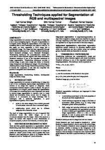
Methods to measure performances. 2.1 Methods that are used now. The now used method can be described as follows. First, there is a scene in the real world. This can be anything, from a rural area to biological cells. A picture is taken, in the case of a rural area, using a satellite or via airborne remote sensing. The resulting picture is used as an input for a segmentation program and it is given to a human expert or a team of human experts. The human expert or the team of human experts makes a segmentation of the picture. This segmentation is considered to be correct and the segmentation that is made by the segmentation program is compared to the segmentation the human expert(s) made. If the segmentation made by the segmentation program, deviates from the segmentation made by the human expert(s), it is said that the computer made segmentation contains errors. It is known that the human made segmentations contain errors. A way to reduce the number of errors made in the human made segmentation, is to gather additional information about the scene the image was made of. In case of a satellite image of a rural area, people can be sent into the elds to measure the elds. Additional information can also be obtained from existing ground maps. The additional information is used to make a more accurate segmentation. If more is known about the scene the image was made of, the segmentation can be made using a greater accuracy. Sometimes gathering additional information is impossible, because it is too expensive, or because there are no ground maps available, or because it is impossible to send people to the scene to inspect the scene itself. The latter reason can be obvious, when the scene is somewhere far away in outer space, or when the scene is too dangerous to send people into, or when images are made of for instance blood cells, seen through a microscope. If additional information is not available, there is a way to reduce the in uence of the errors made in the human made segmentations. A lot of human experts is asked to make a segmentation of the image. The computer made segmentation is than compared to all human made segmentations. The human made segmentations vote for the correctness of the segmentation. If only one human expert assigns a pixel to some region, whereas the other human experts assign the pixel to another region, then probably the human expert has made an error. In a scheme, the method looks as depicted in gure 2.1. 9

CHAPTER 2. METHODS TO MEASURE PERFORMANCES.

10 Objects in real world

Satellite or Airborne Remote Sensing

Segmented

Segmentation

Satellite

Program

Image

Segmentation

Human

"Correct"

Human

Performance

Expert(s)

Segmentation(s)

Expert(s)

Report

Fig 2.1: The now used method.

2.2 Problems with the method. There are some problems that come with the mentioned method:  'Correct' segmentations are made using the remote sensed image. These images contain less information than the scene in the real world. Sometimes additional information is gathered by sending people into the elds, or by using ground maps. Sending people to the scene is not always possible, and ground maps are not always available.  Dierent human experts make dierent correct segmentations, so it is hard to tell what segmentation really is correct.  The segmentation that is to be measured is compared to segmentations that are known to contain errors. It is possible that the computer made segmentation is in fact better than the human made segmentations, but it is said that the computer made segmentation contains errors, since it deviates from the human made segmentations.  There is no generally accepted quantitative measure. A quantitative measure is needed, in order to compare dierent segmentations of the same image.

2.3 A new method. Being aware of the problems with the now used methods and wanting to automatically compare threshold settings used in segmentation programs, there was a need for a method that could automatically measure the error rate of a segmentation. Before one can tell what is wrong, one has to know what is correct. In other words, there was a need for a correct automatically made segmentation of a satellite image. This correct segmentation should be compared to a segmentation made by a segmentation program, so that the error rate of the latter segmentation could be measured. Making the correct segmentation of a satellite image would eliminate the goal of nding the best way to segment a satellite image, because the program that could make a correct segmentation would then have been developed. In this method, another way of knowing the correct segmentation has been developed: not a real satellite image should be used, but an image that looked like a satellite image, but was in fact a simulation of a satellite image. The original data should not be from an agricultural area somewhere on the earths surface, but should be a human made drawing, that was transformed into an image that was

2.4. PROPERTIES OF A SATELLITE IMAGE.

11

indistinguishable from a real satellite image. In that case, images could be generated having properties that were wanted by people doing research on segmentation programs. The original human drawing itself was the correct segmentation! Boundaries of objects, the position of the objects and the properties of the objects were correctly known, because of the simple fact that humans drew them that way! The correct segmentation was not derived from the satellite image, but the satellite image was derived from the correct segmentation. Having the correct segmentation made it possible to fairly and correctly measure the error rate of other segmentations. In short, a correct segmentation should be made. From that correct segmentation, a satellite image should be generated, which should be segmented by the segmentation programs under research. The error rate of the segmentations made by these programs could then be measured using the correct segmentation and a report of the error measurement could be made. Therefore, two programs were developed: Simsat and Qmeasure. Simsat is used to make a correct segmentation out of a human made drawing and Simsat is used to generate a satellite image of the correct segmentation together with some additional object information. Qmeasure is used to measure the error rate of a given segmentation, using the correct segmentation and Qmeasure makes a report of that error rate. Both Simsat and Qmeasure are described in chapter 8. The problem of having the correct segmentation in order to be able to fairly and correctly measure the error rate of a segmentation automatically was solved, but now a satellite image should be generated and it should be indistinguishable from a real satellite image.

2.4 Properties of a satellite image. As an input to segmentation les, a segmented satellite image is used. This le is normally in the ERDAS74 le format, so an image in the ERDAS74 le format was to be generated by Simsat. The ERDAS74 le format is discussed in chapter 4.4. Important is that a satellite image consists of a number of channels, each representing sample values of measures made by dierent sensors. For instance, one can use channels 1 to and 3 for the red, green and blue parts of visible light, channel 4 for infrared light, channel 5 for ultraviolet light and channel 6 for radar data. Objects in the scene, however, re ect light in the total range of the spectrum. Dividing the spectrum into a number of channels, implies dividing the re ection that is typical for a speci c object into a number of channels. The principle of isolating and classifying the dierent objects in an image is based on the fact that dierent elds with dierent crops have dierent characteristics in the dierent channels. For instance, the absorption of light in dierent wavelengths diers from crop to crop. The way crops are sown is dierent for each crop type, resulting in a dierent amount of bare soil between the individual plants. Depending on the resolution used while taking the picture, elds are not smooth, it can be said that they have a mean value, and a standard deviation. When plants in the areas are bigger, or the used resolution is higher, the areas also have a typical texture. In forests, with big trees, one can see the crowns of the trees in the texture of the forest. Objects in scenes have boundaries. These boundaries often coincide within one pixel, if an image is made. The pixel then obtains its value from dierent objects in the scene and the pixel is called a mixed pixel. In short, satellite images of ground data, have properties as:  Dierent crops in elds have dierent values in the dierent channels.

12

CHAPTER 2. METHODS TO MEASURE PERFORMANCES.

 Fields are not smooth, but have a mean value and a standard deviation.  Areas can have texture.  When dierent elds are involved in one picture element, the pixel will be

assigned a value that is in between the values of the individual elds. The pixel will be a mixed pixel.

 There is a correlation between the dierent channels in the image, because

not the objects divide the wavelengths in the spectrum into parts, sensors do.

Simsat is designed to take care of mixed pixels, and to give elds a typical mean values and values for the standard deviation for every channel. These values can be obtained from real satellite images, making the generated images look more like a real satellite image. The dierent channels in the satellite image, can also be given a correlation, by applying a covariance matrix. Fields made by Simsat, however, don't have texture. One could take pieces of elds in real satellite images and use them in the arti cial satellite image, adding texture to the image, but this is left as a future option.

2.5 Summary of the proposed method. Because the now used method is expensive in use and contains errors itself, a new method was developed. This new method no longer uses satellites to take pictures and it no longer makes use of people that are sent into the elds, in order to get some additional information. The proposed method consists of a number of steps:

 First an X11-bitmap picture is drawn by someone. This can be done using

X g. The X11-bitmap format was chosen, because it was simple to read. Reading a human made drawing was not part of the goal of the project, but it was necessary in the method.

 The characteristics le is typed. This can be done using any ASCII editor. The

format of the characteristics le is described in chapter 4. The characteristics le contains the typical characteristics of the objects that are drawn. In future options, it might be possible to refer to "a eld of bare soil" instead of "a eld with this typical values".

 The program Simsat is used to generate a segmented satellite image and a

so called Segref le (Segref stands for Segmentation Reference). The Segref le is used to store information about the objects in the image and is used to derive the correct segmentation. The format is described in chapter 4 and the derivation of the correct segmentation from this Segref le is described in chapter 3.

 The segmentation program that is being tested, is used to segment the satellite

image. The output of this program must be in the REGINF le format. This le format is described in chapter 4.

 The computer made segmentation is compared to the segmentation reference le and a report is made.

In a diagram, the method looks like this:

2.6. DIFFERENCES WITH THE NOW USED METHOD.

13

X11-bitmap

Segmented

Segmentation

drawing

Satellite

program

Image Human

Simsat Correct Field

segmentation

Segmentation

characteristics

Program for performance measurement

Performance report

Fig 2.2: The proposed method.

2.6 Dierences with the now used method. As can be seen in the scheme and as can be read from the description of the method, there are a number of dierences between the new method and the now used method:  The satellite image is not generated using real world objects. A human draws a picture and provides the eld characteristics.  The error rate of the segmentation of the image is not measured using the satellite image, but using the segref le, which contains more information about the elds than the satellite image. From this Segref le a correct segmentation, a standard of what should be done, is derived, to which the computer made segmentation is compared.  No additional ground information is needed, because all available information is contained in the Segref le. The Segref le can be seen as a ground map, where not only the position and the boundaries of the dierent objects in the image are known, but also their typical characteristics.  The correct segmentation can be derived from the original drawing. This segmentation really is correct, in the sense that it is free from errors.  A quantitative scale is used, making it possible to compare dierent segmentations of the same image.

14

CHAPTER 2. METHODS TO MEASURE PERFORMANCES.

Chapter 3

The error measurement in the new method. Before a measurement of the error rate of a segmentation can be made, it must be known when a segmentation contains errors. In order to know when a segmentation contains errors, it must be known what an error is, and what correct is. As the Webster dictionary states: ... . 2. correct k*-'rek-(t)le- 'rek(t)-n*s aj [ME, corrected, fr. L correctus, fr. pp. of corrigere] (a) conforming to an approved or conventional standard (b) conforming to or agreeing with fact, logic, or known truth : ACCURATE (c) conforming to a set gure (as an established price)M, RIGHT mean conforming to fact, standard, or truth. CORRECT usu. implies freedom from fault or error as judged by some standard; ACCURATE implies delity to fact or truth attained by exercise of care; EXACT stresses a very strict agreement with fact, standard, or truth; PRECISE adds to EXACT an emphasis on sharpness of de nition or delimitation; NICE stresses great precision and delicacy of adjustment or discrimination; RIGHT is close to CORRECT but has a stronger positive emphasis on conformity to fact or truth rather than mere absence of error or fault cor.rect.ly av SYN syn CORRECT, ACCURATE, EXACT, PRECISE, NICE er.ror er-*r er-*r-l*s n [ME errour, fr. OF, fr. L error, fr. errare] 1. (a) an act or condition of often ignorant or imprudent deviation from a code of behavior (b) an act involving an unintentional deviation from truth or accuracy (c) i. an act that through ignorance, de ciency, or accident departs from or fails to achieve what should be done ii. a defensive misplay other than a wild pitch or passed ball made by a baseball player when normal play would have resulted in an out or prevented an advance by a base runner 15

16

CHAPTER 3. THE ERROR MEASUREMENT IN THE NEW METHOD.

2. a mistake in the proceedings of a court of record in matters of law or of fact 3. (a) the quality or state of erring Christian Science (b) illusion about the nature of reality that is the cause of human suering : the contradiction of truth (c) an instance of false belief 4. something produced by mistake 5. (a) the dierence between an observed or calculated value and a true value; specif : variation in measurements, calculations, or observations of a quantity due to mistakes or to uncontrollable factors (b) the amount of deviation from a standard or speci cationean a departure from what is true, right, or proper. ERROR may imply carelessness or willfulness in failing to follow a true course or a model, but it may suggest an inaccuracy where accuracy is impossible; MISTAKE implies misconception or inadventence and is seldom a harsh term; BLUNDER commonly implies stupidity or ignorance and usu. culpability; SLIP carries a strong implication of inadventence or accident producing trivial mistakes; LAPSE implies forgetfulness, weakness, or inattention - er.ror.less aj SYN syn ERROR, MISTAKE, BLUNDER, SLIP, LAPSE m err e(*)r, '*r vi [ME erren, fr. OF errer, fr. L errare; akin to OE ierre] wandering, angry, ON ra-s race archaic 1. STRAY 2. (a) to make a mistake (b) to violate an accepted standard of conduct As can be seen from the Webster dictionary, correct usually implies freedom from fault or error as judged by some standard. Freedom of error implies the absence of deviation from a standard or speci cation; a departure from what is true, right or proper. Also, an error is an act that departs from or fails to achieve what should be done. So, in order to measure the error rate of a segmentation, some kind of standard has to be known, something that is true, right or proper, something that should be done. From that standard, the deviation from that standard, or, the occurrence of errors can be judged. In order to develop a standard to which a segmentation of an image must comply, it must be known how the images are made. When making a digital image, the original scene is scanned using sensors. These sensors act as a matrix that is laid over the original scene. Every cell in the matrix contains a piece of the original scene. From the quantity of light, a value is measured, that is lled in a cell in the digital image. When a digital satellite image is made, there are a number of dierent sensors used, which are sensitive to dierent wavelengths of light. For instance, there are sensors that are sensitive to the red, green or blue part of visible light, and there are sensors sensitive to ultraviolet, infrared or radar part of the spectrum. The size of the cells compared to the size of the part of the original scene that ts in the cell, is called the resolution. The smaller the part of the original scene that ts inside one cell, the higher the resolution and the more detail there is in the digital image.

17 The part of the scene that ts in a cell, can consist only of one object, or a part of it, or it can consist of more than one object or parts of objects. The objects can be anything in the original scene. If for instance a picture is made of a rural area, the objects can be plants, cattle, elds, roads, canals or farms. When there are more than one objects involved in the cell in the matrix, the cell is called a mixed cell, or a mixed pixel. The smaller the objects are that are to be isolated, the higher the images resolution must be. If the LANDSAT.TM satellite is used to make an image, one pixel in the image stands for an area of 30 by 30 meters. Since plants and cattle aren't that big, they cannot be isolated. The elds however, are mostly larger than 30 by 30 meters, so they are represented by one or more pixels in the digital image. A segmentation, is a division of the image into segments. These segments represent the objects in the image. The de nition of "objects in the image" is application and scene dependent. It is useful to de ne objects that are larger than a pixel in the image. If the de ned objects are smaller than a pixel in the image, it might be useful to make an image using a higher resolution, so that the objects become larger than the size of a pixel. In this method, a picture is drawn using a drawing utility. The objects in the drawn image have known boundaries and are closed, so the individual objects are known. The drawn image is used as a standard, or as a correct segmentation. In the correct segmentation, all pixels that belong to the same object, are in the same segment, and all pixels that do not belong to this object are in dierent segments. If there is a deviation from the standard, the segmentation contains errors. There are four kinds of errors that can be made in a segmentation:

   

(Parts of) dierent objects are assigned to the same segment. An individual object is split into several segments. A pixel is assigned to several segments. A pixel is not assigned to any segment.

In the arti cially made satellite image, mixed pixels may occur. These mixed pixels have their value obtained from more than one object in the image. In order to make a correct segmentation, without a deviation from the standard, these mixed pixels should be split up into the parts that contributed to the pixels value. These mixed pixels often cause a diculty for the current segmentation programs. The current segmentation programs are not able to correctly split up mixed pixels, or even to split up mixed pixels. As the Webster dictionary states (5. (b)): ERROR may imply carelessness or willfulness in failing to follow a true course or a model, but it may suggest an inaccuracy where accuracy is impossible; Since the current segmentation programs cannot correctly split up mixed pixels, or can't even split up mixed pixels, there is an inaccuracy in the segmentation, where accuracy is impossible. Since accuracy is impossible when using these segmentation techniques, the segmentations are always inaccurate, thus always contain errors. That is, if the standard of what should be done, is the division of (sub)pixels into segments that represent the individual objects in the original scene. The standard of what should be done, can also be de ned in another way. Since the occurrence of mixed pixels is the cause of the impossibility of accuracy, another sub-standard of what should be done with mixed pixels can be de ned. The standard than depends less on the correct segmentation into the objects in the scene, but more on the severeness of the inaccuracy. The severeness of the

18

CHAPTER 3. THE ERROR MEASUREMENT IN THE NEW METHOD.

inaccuracy in segmenting mixed pixels is application dependent. In one application certain kinds of errors are more severe than in other applications. And certain kind of errors can be more severe than other kinds of errors. If for instance, a segment is beyond the focus of attention, errors might be less severe. The correctness of a segmentation then depends more on the classi cation of the pixels in the image and on the usability and acceptability of the segmentation. It is application dependent what segmentation is better and what segmentation is worse. Mostly, the segmentation of pixels that obtained their values from only one object must be assigned to segments that represent the objects in the original scene. The mixed pixels however, can have dierent, application dependent requirements. Requirements for mixed pixels can be: 1. Mixed pixels should be merged with the segment, that represents the object that contributed the most to the value of the pixel. 2. Mixed pixels should be recognized as mixed pixels and should be segmented in own segments. 3. Mixed pixels have their values obtained from several objects. The combinations of objects form pixel classes. These dierent classes should be dierent segments in the segmentation. 4. Mixed pixels are not important, since they always contain errors. Mixed pixels should thus be neglected during the performance measure. Making a standard of what should be done, implies knowing what should be done. That what should be done, is application dependent, and must be known before a measurement on the occurrence of errors can be done. If the satellite image is known to subpixel level, it is known whether a pixel is mixed or not, and to what object the pixel belongs. If the pixel is a mixed pixel, it is known what objects contributed to its value, and it is known what subpixels belong to what object in the scene. Then, if the requirements for the mixed pixels are known, it is possible to make a standard of what should be done. In order to make a distinction between the objects in the original scene, and the segments that are wanted in the standard of what should be done, target objects are introduced. Target objects are the dierent individual segments that are wanted in the segmentation of the image. The target objects mostly are:  Segments containing all full pixels of one individual scene object, with or without the subpixels from that scene objects that contributed to the mixed pixels.  Segments that contain only mixed pixels, according to the requirements that are stated for the mixed pixels. If mixed pixels should be split up, there should be no segments containing mixed pixels in the standard of what should be done.

3.1 Comparing the segmentation to the standard. In order to measure the error rate of a segmentation, the segmentation must be compared to the standard of what should be done. The found segments must be compared to the target objects. Target objects and segments both contain pixels, and in order to compare target objects and segments, the pixels in the target objects and the pixels in the found segments must be compared. If pixels in dierent les and in dierent formats are to be compared, it must be known, what pixels can be compared to one and other. In the generation of the

3.1. COMPARING THE SEGMENTATION TO THE STANDARD.

19

segmented satellite image, subpixeling is used. A block of pixels is used to determine the value of one pixel in the satellite image. The resolution of the segmented satellite image is lower than the resolution in the human made drawing. If the segmentation program can't split up mixed pixels and can either assign a pixel to a segment or not assign a pixel to a segment, the resolution of the segmentation is the same as the resolution of the segmented satellite image, and therefore lower than the human made drawing. Therefore, in the image that has the higher resolution, a block of pixels is compared to a pixel in the image that has the lower resolution. Pixels can be compared to one and other, if they correspond to one and other.

De nition: A pixel in the original image corresponds to a pixel in the segmentation, if the coordinates of the pixel in the original image correspond to the coordinates of the pixel in the segmentation. If the resolutions of both images are the same, the coordinates of the corresponding pixels are the same. If the resolution of the images are dierent, then the larger image, which is usually the original segref le, obtained from the X11-bitmap image, is divided into super-pixels. The number of super-pixels in the larger image must be the same as the number of pixels in the smaller image, because both the number of super-pixels in horizontal direction as the number of super-pixels in the vertical direction in the larger image must be the same as the number of pixels in the horizontal direction and the number of pixels in the vertical direction of the smaller image respectively. Then, a pixel in the larger image corresponds to a pixel in the segmentation, if the coordinates of the super-pixel of which the pixel is part of, are the same as the pixel in the smaller image. As an example: a pixel in the larger image, that is part of the third super-pixel on the second line, corresponds to the third pixel on the second line in the smaller image. In the next pages of this thesis, will be spoken of the same pixel in the original image as in the segmentation, if both pixels correspond to each other. If it is known what pixels can be compared to one and other, and it is known what pixels belong to what target objects and what pixels belong to what found segments, target objects can be compared to found segments. In the SEGREF le, the target objects can be labeled, so that each target object has a unique label. This is already done for the pixels belonging to the scene objects, and has to be redone if target objects and scene objects are not the same. For instance, when mixed pixels cannot be split up and have dierent requirements. According to the requirements, the dierent target objects can be recognized and labeled. The found segments are distinguishable, so they can be labeled with unique numbers. Comparing the target objects and the found segments can then be done by comparing the target objects labels and the found segments labels. In order to measure the deviation from the standard, it is sucient to count the number of occurrences of a combination of a target object label and a found segment label. This is done by using a set of triples.  A triple < target object id; found segment id; numpix >, consists of three

natural numbers; target object id, found segment id and numpix. A triple describes a combination of these three natural numbers. A label of a target object is denoted by the number target object id, the label of a found segment, is denoted by the number found segment id and the number numpix refers to the number of corresponding pixels that have label target object id in the standard of what should be done and found segment id in the found segmentation. The dierent parts of a triple t can be selected by a set of selecting operators: { O(t) selects the target-object-id part of the triple t. { S(t) selects the found-segment-id part of the triple t.

20

CHAPTER 3. THE ERROR MEASUREMENT IN THE NEW METHOD.

{ N(t) selects the numpix part of the triple t. The set of triples is made by starting with an empty set S and then reading every segment in the segmentation, one at a time. Then, for every pixel in the segment, the pixels in the correct segmentation, that contributed to the pixels value, are read. For every read pixel in the correct segmentation, the number of occurrences of the dierent target object labels are counted. If the pixel is a mixed pixel, the target objects can be dierent from the original labels. At this point, the target object labels, the segment labels and the number of (sub)pixels are known, and triples are made. The triples are then used to update the set. Updating the set S with a triple t is done using the following rules:  If the set S contains no triples t0 with O(t) = O(t0 ) and S(t) = S(t0 ), then triple t is added to the set.

 If the set S contains a triple t0 with O(t) = O(t0 ) and S(t) = S(t0 ), triple t0 is

deleted from the set S. A new triple < O(t); S(t); N(t) + N(t0 ) > is added to the set S. When all pixels have been processed, the set contains a comparison of the standard of what should be done and the found segmentation. The set consists of triples, all with a unique combination of target object labels and found segment labels. For every combination of target object labels and found segment labels, the number of pixels, that have that combination, is also contained in the triple. Further, the number of pixels in the dierent target objects is known; all pixels in the same target objects are counted in triples that have the same target object id part. In the same way, the number of pixels in the dierent found segments is known. Also, it is known, what number of pixels that should be in the same target object, are assigned to what found segments and vice versa, making the comparison complete. Because a rated error is desired, from the comparison an error rate must be calculated.

3.2 Calculating the error rate. When the standard of what should be done has been compared to the found segmentation, a rated error can be calculated. From the set of triples, the deviation from the standard of what should be done, can be seen. If the set contains triples t and t0 with S(t) = S(t0 ), but O(t) 6= O(t0 ), (part of) target objects are merged in the found segmentation, since there are pixels that are in the same segment in the found segmentation, but are in dierent target objects in the standard of what should be done. If on the other hand, the set contains triples t and t0 with S(t) 6= S(t0 ), but O(t) = O(t0), (part of) target objects are split into more than one segments, since there are pixels that are in the same target object in the standard of what should be done, but are in dierent found segments in the found segmentation. That is, if N(t) 6= 0 and N(t0 ) 6= 0. But from the method used to obtain the set of triples, it can be seen, that the set contains no triples t with N(t) = 0. In order to give a rated error measure, the following functions were developed, according to two main ideas: 1. A recursive idea, where the quality of a segment is the amount of correctly assigned pixels multiplied by the quality of the other pixels in the segment (see section 4.2). The developed functions for this idea are:

 The merge quality (QMerge), to measure incorrectly merged (parts of) target objects.

3.2. CALCULATING THE ERROR RATE.

21

 The split quality (QSplit), to measure incorrectly split (parts of) target

objects.  The overall merge quality (Overall QMerge), average of Qmerge for every segment.  The overall split quality (Overall QSplit), average of QSplit for every target object.  Overall performance, average of Overall QSplit and Overall QMerge. 2. Since according to the Webster dictionary, noise is: 2b: an unwanted signal in an electronic communication system obs Errors are a deviation from a standard of what should be done and are therefore unwanted. Errors in a segmentation can thus be considered as noise. The process of segmenting an image, can be seen as a process, that translates the image into a standard of what should be done. This standard is then sent by a sending entity to a receiving entity. The receiving entity receives the segmentation of the image. If the used channel is noiseless, the standard of what should be done is received and the segmentation contains no errors. If the used channel, however, is not noiseless, noise is added during the transmission, resulting in a segmentation that deviates from the standard. Splitting objects can then be seen as adding information (in information theoretic sense) to the standard, resulting in an image that contains more information. Merging objects can be seen as loss of information, resulting in a segmentation, that contains less information. Loss of information during the transmission of the standard, compares to adding information during the transmission of the segmentation. The sending entity sends the segmentation to the receiving entity, that receives the standard of what should be done. During the transmission noise is added, resulting in a standard that contains more information than the segmentation. The amount of noise added during the transmission, resulting in both loss and addition of information, compares then to the error rate of the segmentation (see section 4.3). The developed functions for this idea are:  The merge entropy, to measure to amount of noise added when merging objects .  The overall merge entropy, average of the merge entropy for every segment.  The split entropy, to measure the amount of noise added when splitting objects.  The overall split entropy, the average of the split entropy for every object.  The mean entropy, to measure the average amount of noise added when converting target objects to segments and vice versa. In the dierent functions, some general properties of the set of triples, containing the comparison of the standard of what should be done and the found segmentation, are used.  A target object o is split, if the set of triples S, contains triples t and t0, with N(t) 6= 0, N(t0 ) 6= 0, S(t) 6= S(t0 ), but O(t) = O(t0 ). There are dierent triples with the same target object id.  Target objects are merged into a segment s, if the set of triples S, contains triples t and t0, with N(t) 6= 0, N(t0 ) 6= 0, O(t) 6= O(t0 ), but S(t) = S(t0 ). There are dierent triples with the same found segment id.

22

CHAPTER 3. THE ERROR MEASUREMENT IN THE NEW METHOD.

 The total number of pixels that is assigned to a segment s is equal to P N(t) tS jS t s ( )=

 The total number of pixels that should be in one target object o is equal to P tS jO t o N(t) ( )=

 The number of pixels that are assigned to a segment s and should be in target o, is equal to P

tS jO t o^S t s N(t) ( )=

( )=

Since there is only one triple t in the set S, with O(t) = o and S(t) = s, the number of pixels that are assigned to a segment s and should be in target o, is equal to N(t) of that triple.

3.2.1 The recursive idea.

The recursive idea, is based on the idea that the largest number of pixels that are assigned to a segment s, and should be in a target object t, is correctly segmented. The other pixels should be in another target object and should thus be assigned to another segment. They form (a part of) a target object that was incorrectly merged with the segment. Or, the other pixels should be in the same target object, but were assigned to another segment or to several other segments. In this case the target obect was incorrectly split. Splitting or merging depends on the role segments and target objects play. If the number of correctly segmented pixels is equal to the total number of pixels in a segment or in a target object, the segment or target object itself is correctly segmented. If, on the other hand, only a part of the total number of pixels in the segment, or in the target object, is correctly segmented, then the other pixels are incorrectly segmented. The quality of a segmentation then depends on the percentage correctly segmented pixels, multiplied by the quality of the incorrectly segmented pixels. The quality of the incorrectly segmented pixels is considered to be better, when the incorrectly segmented pixels are assigned to only one incorrect segment, than when they are assigned to several incorrect segments.

QMerge.

Target objects, or parts of target objects, can be incorrectly merged with (parts of) other target objects. If they are incorrectly merged, they are assigned to the same segment, when they should be assigned to dierent segments. In order to measure the merge quality of a segment, that is, the quality depending on incorrectly merged (parts of) target objects into one segment, the number of pixels in the segment, to what target objects they should be assigned and the number of pixels in the target objects that were assigned to the segment must be known. Therefore, a subset Ss of the comparison set S is made, Ss = ftS jS(t) = sg, containing all triples t, that describe a number of pixels assigned to the segment with segment label s. The set is descendingly sorted, according to the numpix parts of the triples, so that the triple with the largest numpix part N(t) comes rst. Then, the triples can be numbered, according to their position in the sorted set, the rst triple is called t , the second triple is called t and so on, until tnumtriples, where 1

2

3.2. CALCULATING THE ERROR RATE.

23

numtriples is the number of triples in the sorted set. Then, 8j; k; j < k : N(tj )  N(tk ). Then the quality Q of a set is de ned as: QMerge(EmptySet) = 1 N(t ) QMerge(Ss ) = TotalNumpix(S )  Q(Ss ? t )

(3.1) (3.2) (3.3)

1

s

1

Since

 TotalNumpix(Ss ? t ) = TotalNumpix(Ss ) ? N(t ) 1

1

 the rst triple in the sorted set Ss ? t is the same as the second triple in the 1

sorted set Ss

 during the recursion, the set gets smaller, and eventually empty, the recursion ends with QMerge(EmptySet) = 1

the formula can be unfolded [3], or written without recursion, as follows: N(t ) N(t ) QMerge(Ss ) = TotalNumpix(S
TotalNumpix(S
) s s ) ? N(t ) N(t ) TotalNumpix(Ss ) ? N(t ) ? N(t )
:::
N(tnumtriples) TotalNumpix ? N(t ) ? N(t ) ? ::: ? N(tnumtriples? ) 1

2

1

3

1

1

2

2

1

where numtriples is the number of triples is the sorted set Ss . The quality of a segment in the segmentation, depends on the percentage correctly segmented pixels. This percentage is multiplied by the quality of the rest of the pixels in the segment. Another possibility is to have a quality measure, where the quality of the incorrectly segmented pixels is not taken into account. The other pixels are not correctly segmented anyway. This possibility was not chosen, in order to be able to compare dierent segmentations, with the same percentage of correctly segmented pixels. A segmentation is better, if it merges less (parts of) target objects into one segment.

Overall QMerge. When for every segment s, the merge quality has been calculated, the overall merge quality can be calculated. This is done by simply taking the average of all merge qualities. Every segment has the same weight in the average. Another possibility is to weight the merge qualities with the number of pixels in the segment. This possibility was not chosen, because all target objects have the same meaning, independent of the number of pixels they have. In order to make a correct segmentation, all target objects have to be correctly merged. So OverallQmerge =

QMerge(Ss1 ) + QMerge(Ss2 ) + ::: + QMerge(Ssnumsegments ) numsegments

where numsegments is the total number of segments in the segmentation and the si 's are the dierent found segment labels.

24

CHAPTER 3. THE ERROR MEASUREMENT IN THE NEW METHOD.

QSplit. Target objects can also be split into a number of segments. If a target object is split, a number of pixels that should be assigned to one target object is assigned to several segments. In order to measure the split quality of a target object, the number of pixels that should be in the target object, the segments the pixels were actually assigned to, and the numbers of pixels that were assigned to the segments, but should be assigned to the target object, must be known. Therefore, just as is done while measuring the merge quality, a subset So of the comparison set S is made, So = ftS jO(t) = og, containing all triples t, that describe a number of pixels that should be assigned to the target object with target object label o. Again, the set needs to be descendingly ordered. The contents of the set is actually the only dierence with the merge quality. From a sorted set So , the split quality is calculated the same way as is done when calculating the merge quality. QSplit(EmptySet) = 1 N(t )  Q(So ? t ) QSplit(So ) = TotalNumpix(S o) 1

1

This function is actually the same as the QMerge function, but now So is used instead of Ss . The role segments and target objects play is now reversed, resulting in dierent sets of triples.

Overall QSplit. When for every target object o, the split quality is calculated, the overall split quality can be calculated. This is done by simply taking the average of all split qualities. Every target object has the same weight in the average. Another possibility is to weight the split qualities with the number of pixels in the segment. This possibility was not chosen, because of the same reason as in calculating the overall merge quality. OverallQSplit =

QSplit(So1 ) + QSplit(So2 ) + ::: + QSplit(Sonumtargets ) numtargets

where numtargets is the total number of target objects in the standard of what should be done and the oi's are the dierent target object labels.

Overall performance. The overall performance is calculated by taking the average of the overall split quality and the overall merge quality. The merge quality and the split quality are considered to be equally important for the overall performance of a segmentation, so the weights for both the split quality and the merge quality in calculating the overall performance must be equal. Therefore OverallPerformance = OverallQSplit +2OverallQMerge

3.2. CALCULATING THE ERROR RATE.

25

Analysis of the function.

In this section, the function for calculating the split quality and the merge quality is analyzed. This is done, by describing the use of the function in calculating the merge quality. Note that the function used in calculating the split quality and the function used in calculating the merge quality are the same. Best case, all pixels that are assigned to a segment, are from one target object. Then, the merge quality will be nn1 = nn = 1. Worst case, all pixels in the segment should be in dierent target objects. Then, all ni s are equal to 1 and the merge quality is equal to n  n?  n?  :::  = n . In all other cases, which are not as good as the best case and which are better than the worst case, the merge quality is between the merge quality in the best case and the merge quality in the worst case. Therefore, the merge quality is between 1 and n . The function has an upper bound of 1, and a lower bound of lim 1 = 0 n!1 n! . The number of ways target objects can be merged into one segment, is equal to the number of ways to divide n pixels into a number of dierent sorted classes, where the next class has a less or equal number of elements and where no class is empty. If the merge qualities for the dierent distributions are calculated, the distributions can be sorted to their error rate. The best case has quality 1 and worst case has quality n . There is only one best case and only one worst case, but there can be multiple cases in between that have an equal merge quality. These cases are considered to be equally correct and equally incorrect. 1

1

1

1

1

2

1

1

!

1

!

1

!

3.2.2 Using the entropy as an error measure.

A segmentation technique transforms an image containing objects into a chain of objects, forming an image. In order to have a correct segmentation, the objects found by the segmentation technique, must correspond to the target objects de ned in the standard of what should be done. The dierent target objects can be labeled with unique labels and the regions found by the segmentation program can also be labeled with unique labels. If the segmentation is correct, then pixels that belong to the same target object in the standard of what should be done must be assigned to the same segment in the segmentation. All pixels that are in dierent target objects in the standard of what should be done must be in dierent segments in the segmentation. Thus all pixels in the standard of what should be done, that have the same labels must have the same labels in the segmentation and pixels having dierent labels in the original image must have dierent labels in the segmentation. The process of segmenting a digital image can be seen as a communication process between a sending entity that rst segments the digital image correctly to the standard of what should be done, and then sends the target objects over a certain channel to a receiving entity, that receives the segments in the segmentation. If the channel is noiseless, the received segments are the same as the sent target objects, so that the standard of what should be done is received. The segmentation is then free of errors. If however, the channel is not noiseless, noise is added to the signal, resulting in a received segmentation that deviates from the standard of what should be done and that therefore contains errors. The amount of noise added to the signal can then be used as an error measure. In a segmentation, target objects, or parts of target objects, can be incorrectly merged. If (parts of) target objects are incorrectly merged, some pixels that should

26

CHAPTER 3. THE ERROR MEASUREMENT IN THE NEW METHOD.

have dierent labels are given the same labels. This results in a decrease of information (in information theoretic sense), and results thus in a decrease in the entropy, because the standard of what should be done contains more dierent labels in that part of the image, than the found segmentation does. If (parts of) target objects or incorrectly split, pixels that should have the same label, are assigned dierent labels. The segmentation contains more dierent labels in that part of the image than the standard of what should be done. This causes an increase of information in that part of the image, and results thus in an increase of the entropy. In the same segmentation, both kind of errors can be made. A decrease in the entropy caused by incorrectly merging some (parts of) target objects, followed by an increase in the entropy caused by incorrectly splitting some (parts of) target objects, can cause the entropy in the segmentation to be the same as the entropy in the standard of what should be done. The segmentation should then appear to be correct, but it actually contains two errors. Therefore, the following functions were developed:  The split entropy, to measure the average amount of information added per pixel in a target object, caused by splitting target objects.

 The overall split entropy, to measure the average amount of added information per pixel per target object added when splitting target objects.

 The merge entropy, to measure the average amount of information lost per pixel in a segment, caused by merging target objects.

 The overall merge entropy, to measure the average amount of lost information per pixel per segment when merging target objects.

 The overall entropy, to measure the average amount of noise added in the segmentation.

The split entropy. When splitting an object into a number of dierent segments, a number of pixels having the same labels in the original image are given dierent labels in the segmentation. In the segmentation of the target object, there is a larger number of dierent labels than there are in the original target object. According to Shannon[2], the segmentation of the target object contains more information than the original image. The amount of information in the segmentation can be calculated when the probabilities pi of a transmitted label being label i are known. The average amount of information per pixel equals to the entropy H, which is de ned by Shannon [2] as:   n X pi
log p1 i i 2

=1

where n is the number of dierent labels in the region, and pi is the probability of a transmitted label being label i. Because log is used, the value of H is expressed in bits per pixel. The average amount of added information per pixel in the segmentation of a target object equals to the average amount of information per pixel in the segmentation of the target object minus the average amount of information per pixel in the target object. In a formula: The average amount of added noise per pixel E = H(segmentation of the object) ? H(original object) 2

3.2. CALCULATING THE ERROR RATE.

27

Because all pixels in the same object have the same labels, the probability of a label in the same object being the objects label is equal to 1. The probability of a label in the object being another label than the objects label is equal to zero. Thus the information contained in the original object is equal to 1  log( ), which is equal to zero. E is thus equal to H(segmentation of the object). If a set of triples S is made, just like is done according to the recursive idea, Soi = ftS jO(t) = ig X TotalNpix(Soi ) = N(t) 2

1

1

tSoi

X

TotalNpix(Soi ) ) N(t)
log( N(t) tSoi TotalNpix(Soi ) Soi contains all triples describing the segmentation of a target object i. Therefore, E(Soi ) = H(segmentation of the object). In the recursive idea, a correct segmentation has an error rate measure equal to one. A worse segmentation has a lower value. In the idea using the entropy, was chosen to have the same value for the correct segmentation, and to have a lower value for a worse segmentation. Therefore E(Soi ) =

2

Esplit(Soi ) = 1 ? E(Soi )

the overall split entropy.

The overall split entropy is derived from the average amount of added noise per pixel per target object. The E(Soi )s describe the average amount of added noise per pixel in a target object i. The average amount of added noise per pixel per segment E 00 equals then to TotalObjects X 1 E(Soi ) E 00 = TotalObjects i =1

where TotalObjects is the total number of target objects in the standard of what should be done. Again, in order to have the best segmentation given the value one, and to give a worse segmentation a lower value, the overall split entropy is de ned as: TotalObjects X 1 OverallESplit = 1 ? TotalObjects E(Soi ) i =1

The merge entropy.

The merge entropy is used to measure the amount of information that is lost, because of an incorrect merging of target objects. If a segment in the segmentation, consists of (parts of) dierent target objects that are incorrectly merged, pixels that should have dierent labels, are given the same label. In the segment, there are less dierent labels than there are in the set of corresponding pixels in the standard of what should be done. The average amount of information per pixel that is lost, can be calculated using the entropy. The amount of lost information, is equal to the information contained in the pixels that correspond to the segment minus the information contained in the segment itself. In a formula: E 0 = H(f pixels corresponding to segment i g) ? H( segment i )

28

CHAPTER 3. THE ERROR MEASUREMENT IN THE NEW METHOD.

Since all pixels in the segment have the same label, H(segment i) = 0, so E 0 = H(fpixels corresponding to segment ig) Again, a set of triples S can be made, containing the comparison between the segmentation and the standard of what should be done. Then, Ssi = ftS jS(t) = ig X TotalNPix(Ssi ) = N(t) E 0 (Ssi ) =

tSsi

 TotalNpix(S )  N(t) si
log ) TotalNpix(S N(t) s i tSsi X

2

Ssi contains all triples describing the segment i and the corresponding pixels in the standard of what should be done. Therefore, E 0 (Ssi ) = H(pixels corresponding to segment i). In the recursive idea, a correct segmentation has an error rate measure equal to one. A worse segmentation has a lower value. In the idea using the entropy, was chosen to have the same value for the correct segmentation, and to have a lower value for a worse segmentation. Therefore Emerge (Ssi ) = 1 ? E 0(Ssi )

The overall merge entropy. The overall merge entropy is derived from the average amount of added noise per pixel per segment. The E 0 (Ssi )s describe the average amount of added noise per pixel in a segment i. The average amount of added noise per pixel per segment E 000 equals then to TotalSegments X 1 E 000 = TotalSegments E 0 (Ssi ) i =1

Again, in order to have the best segmentation given the value one, and to give a worse segmentation a lower value, the overall merge entropy is de ned as: TotalSegments X 1 OverallEmerge = 1 ? TotalSegments E(Ssi ) i =1

where TotalSegments is the number of segments in the segmentation.

The overall entropy. The overall entropy is de ned as OverallEntropy = OverallEMerge(S)2+ OverallESplit(S) In order to have a correct segmentation, all target objects must be correctly segmented. Incorrectly merging and incorrectly splitting are considered to be equally important to a correct segmentation. Therefore, the weights of the OverallMergeEntropy and the OverallSplitEntropy are the same.

3.2. CALCULATING THE ERROR RATE.

29

Analysis of the entropy function

The entropy function is used to measure the amount of information in a string. The string is sent by a source and consists of symbols from an alphabet. The symbols in the alphabet are the only symbols that can be sent by the source. The amount of information in a string, depends on the predictability of the source. The entropy function is de ned by Shannon as: P H = ni pi
log pi where n is the size of the alphabet and pi is the probability of word i in the alphabet to occur. The function H calculates the average amount of bits minimally needed to code a string. The function H has a maximum, if the randomness of the source sending strings is maximum, so that predicting the source is most dicult. The randomness of the source is at a maximum, if the probabilities of all words in the alphabet are equal, n . The function H is then equal to: P H = ni n
logn = log n If n gets bigger, the maximum of H gets bigger, and if n gets smaller, the maximum of H gets smaller. H has an upperbound of log(n), which depends on n. If n is variable, it is said that H has no upperbound. Since ESplit and EMerge are de ned as ESplit(Soi ) = 1 ? H(Soi ) EMerge(Ssi ) = 1 ? H(Ssi ) 2

1

=1

1

1

2

2

=1

2

it can be said that ESplit and EMerge have no lower-bound. Note that QSplit and QMerge have a lower bound of n . If n gets very large, it can be seen that QMerge and QSPlit have a lower bound of lim 1 = 0 n!1 n! The entropy function H gets a minimum, if the source is highly predictable, if the source sends strings consisting only one word in the alphabet. The probability of that word is equal to 1 and the probabilities of other words is equal to 0. The function H is then equal to H = 0
log 0 + :::: + 1
log1 + 0
log 0 + ::: + 0
log0 = 0 If the source is not highly random and is not highly predictable, the function H has a value in between 0 and log n. Note that the functions QSplit and QMerge are in between n and 1. Since n, the size of the alphabet, depends on the size of the objects for the split entropy and on the size of the regions for the merge entropy, the maximum of H and thus the maximum of E depends on the size of the objects or the regions. If a target object contsists of n pixels, n dierent labels can be sent. All pixels in the target object are then given a dierent label. The size of the alphabet is then equal to n. When a larger object is heavily split, the error rate gets to log n with n a larger number. This causes a worse performance of the segmentation than a smaller heavily split object. 1

!

2

2

2

2

2

1

!

2

3.2.3 Example.

In gure 3.1 (a), a drawing is depicted. In gure 3.1 (b) the same drawing can be found, after it has been labeled. In the image, cells can be seen. These cells

30

CHAPTER 3. THE ERROR MEASUREMENT IN THE NEW METHOD.

(a)

1

1

1

0

0

2

2

2

2

1

0

0

5

5

0

0

2

2

0

5

5

5

5

5

5

0

2

0

5

5

5

5

5

5

5

0

0

5

5

5

5

5

5

5

0

4

0

0

5

5

5

5

5

0

4

4

4

0

5

5

5

0

3

4

4

4

4

0

5

0

3

3

4

4

4

4

4

0

3

3

3

(b)

Figure 3.1: An original drawing, with the drawing in (a) and the labels in (b). are labeled with labels, referring to the dierent objects in the scene. In the scene that was drawn, there are ve objects, and they are labeled with numbers from one to ve. There are cells that are labeled with a zero. These cells are boundary cells in the X11-bitmap image, depicted as black pixels in the drawing in gure 3.1 (a). During the generation of the segmented satellite image, as well as in the error measuring, these cells are not taken into account. Further, there are thick lines in the image. These thick lines enclose a super-pixel, which in this example contain a three by three pixels block. The super-pixels in the image, correspond to the pixels in the segmented satellite image, and if the resolution in the segmentation is the same as the resolution in the segmented satellite image, the super-pixels correspond to the pixels in the segmentation. If a pixel in the segmented satellite image, obtains its value from more than one object in the original scene, the pixel is called a mixed pixel. Since a pixel in the segmented satellite image corresponds to a super-pixel in the original drawing, a mixed super-pixel contains cells with dierent labels. Since the cells labeled with a zero are not taken into account, they are not considered to be labeled with a dierent label. The third super-pixel in the second line of super-pixels, contains only cells labeled with zero and cells labeled with ve. The zero labels are not counted, so this super-pixel is not a mixed cell. The super-pixel in the center and the leftmost super-pixel in the bottom line of super-pixels, contain cells that are all labeled with the same label. These super-pixel are also not mixed. The other super-pixels all contain cells labeled with more than one label. These super-pixels are the mixed pixels in the segmented satellite image. Suppose in Figure 3.2 a segmentation of this image is depicted.

1

2

3

2

2

2

4

5

6

Fig 3.2: The segmentation made of Fig 3.1. Then, if mixed pixels should be split up, the triples are: < 1; 1; 4 > < 5; 1; 2 > < 2; 3; 6 > < 5; 3; 1 > < 4; 4; 9 > < 4; 5; 3 > < 5; 5; 3 > < 5; 6; 1 > < 3; 6; 6 > < 2; 2; 1 > < 4; 2; 1 > < 5; 2; 24 > < 0; 1; 3 > < 0; 2; 10 > < 0; 3; 2 > < 0; 5; 3 > < 0; 6; 2 >

3.2. CALCULATING THE ERROR RATE.

31

The total number of pixels in the image is 4 + 2 + 6 + 1 + 9 + 3+ 3 + 1 + 6+ 1 + 1 + 24 + 3 + 10 + 2 + 3 + 2 = 81 = 9
9, the size of the image. The cells labeled with zero, are not taken into account, so the triples are not taken into account either. The set S, is then S = f< 1; 1; 4 >; < 5; 1; 2 >; < 2; 3; 6 >; < 5; 3; 1 >; < 4; 4; 9 >; < 4; 5; 3 >; < 5; 5; 3 >; < 5; 6; 1 >; < 3; 6; 6 >; < 2; 2; 1 >; < 4; 2; 1 >; < 5; 2; 24 >g and TotalNumpix(S) = 61 The dierent subsets of S are: Ss1 = ftS jS(t) = 1g Ss2 = ftS jS(t) = 2g Ss3 = ftS jS(t) = 3g Ss4 = ftS jS(t) = 4g Ss5 = ftS jS(t) = 5g Ss6 = ftS jS(t) = 6g So1 = ftS jO(t) = 1g So2 = ftS jO(t) = 2g So3 = ftS jO(t) = 3g So4 = ftS jO(t) = 4g So5 = ftS jO(t) = 5g

= = = = = = = = = = =

f< 1; 1; 4 >; < 5; 1; 2 >g f< 5; 2; 24 >; < 2; 2; 1 >; < 4; 2; 1 >g f< 2; 3; 6 >; < 5; 3; 1 >g f< 4; 4; 9 >g f< 4; 5; 3 >; < 5; 5; 3 >g f< 3; 6; 6 >; < 5; 6; 1 >g f< 1; 1; 4 >g f< 2; 3; 6 >; < 2; 2; 1 >g f< 3; 6; 6 >g f< 4; 4; 9 >; < 4; 5; 3 >; < 4; 2; 1 >g f< 5; 2; 24 >; < 5; 5; 3 >< 5; 1; 2 >; < 5; 3; 1 >; < 5; 6; 1 >g

Note that the sets are descendingly sorted. According to the two ideas on measuring the error rate, the error rates are:  According to the recursive idea: QMerge(Ss1 ) = 64
22 = 23 24
1
1 = 6 QMerge(Ss2 ) = 26 2 1 13 6 1 QMerge(Ss3 ) = 7
1 = 67 QMerge(Ss4 ) = 99 = 1 QMerge(Ss5 ) = 36
33 = 12 QMerge(Ss6 ) = 76
11 = 67 + + +1+ + 2449 = 3276 OverallQMerge(S) = 6 QSplit(So1 ) = 44 = 1 QSplit(So2 ) = 67
11 = 67 QSplit(So3 ) = 66 = 1 2

6

6

1

6

3

13

7

2

7

32

CHAPTER 3. THE ERROR MEASUREMENT IN THE NEW METHOD. 9
3
1 = 27 QSplit(So4 ) = 13 4 1 52 3 18 24 QSplit(So5 ) = 31
7
24
21
11 = 217 1+ +1+ + 7807 OverallQSplit(S) = = 11284 5 +  0:719711 OverallPerformance(S) = 2 6

27

18

7

52

217

2449

7807

3276

11284

 Using the entropy: EMerge(Ss1 ) = 1 ? 23 log( 23 ) ? 31 log(3) 13 ) ? 1 log(26) 1 log(26) EMerge(Ss2 ) = 1 ? 12 log( 13 12 26 26 1 7 6 EMerge(Ss3 ) = 1 ? 7 log( 6 ) ? 7 log(7) EMerge(Ss4 ) = 1 ? 99 log( 99 ) = 1 ? 0 = 1 EMerge(Ss5 ) = 1 ? 12 log(2) ? 21 log(2) = 0 EMerge(Ss6 ) = 1 ? 67 log( 67 ) ? 71 log(7) 13 OverallEMerge(S) = 16
(6 ? 23 log( 23 ) ? 31 log(3) ? 12 13 log( 12 ) ? 1
log(26) ? 1
log(26) ? 6 log( 7 ) ? 26 26 7 6 1 log(7) ? 1 log(2) ? 1 log(2) ? 6 log( 7 ) ? 7 2 2 7 6 1 log(7))  0:5950 7 2

2

2

2

2

2

2

2

2

2

2

2

2

2

2

2

2

2

2

2

2

2

2

ESplit(So1 ) = 1 ? 44
log( 44 ) = 1 ESplit(So2 ) = 1 ? 67
log( 67 ) ? 17
log(7)  0:4083 ESplit(So3 ) = 1 ? 66
log( 66 ) = 1 9
log( 13 ) ? 3
log( 13 ) ? 1
log(13) ESplit(So4 ) = 1 ? 13 9 13 3 13  0:1401 31 3 31 2 31 ESplit(So5 ) = 1 ? 24 31
log( 24 ) ? 31
log( 3 ) ? 31
log( 2 ) ? 1 1 31
log(31) ? 31
log(31)  ?0:1866 OverallESplit(S)  0:4724 OverallEntropy(S)  0:5337 2

2

2

2

2

2

2

2

2

2

2

2

In the segmentation that is to be measured (see Fig 3.2), mixed pixels were not split up. The fact that mixed pixels were not split up, but should be split

3.2. CALCULATING THE ERROR RATE.

33

up according to the standard of what should be done, caused an unavoidable disagreement between the segmentation and the standard. The segmentation contains errors, because of an inaccuracy where accuracy was impossible. Therefore, some extra requirements for the mixed pixels can be stated, instead of that they should be split up. According to the requirements described in this chapter, the following standards can be made:

Requirements for mixed pixels 1)

Mixed pixels should be merged with the segment, that represents the object that contributed the most on the value of the pixel. In the original drawing where object labels are known to subpixel level, all superpixels have a label that has a majority in the super-pixel, except for one super-pixel: the middle super-pixel in the last row. Label 4 occurs three times, as well as label 5. Therefore, two standards of what should be done can be made. One where the pixel should be in the same segment as the pixels labeled with the label 4, and one where the pixel should be in the same segment as the pixels labeled with label 5.

1

2

3

1

2

3

2

2

2

2

2

2

4

4

5

4

2

5

(a)

(b)

Figure 3.2: Fig 3.3: Standards according to requirements 1) Considering the same segmentation as in gure 3.2, two sets of triples can be made in the comparison between the made segmentation and the two standards of what should be done. 1. According to the standard in gure 3.3 (a): S = f< 1; 1; 1 >; < 2; 2; 4 >; < 3; 3; 1 >; < 4; 4; 1 >; < 4; 5; 1 >; < 5; 6; 1 >g and TotalNumpix(S) = 9 The dierent subsets of S are: Ss1 = ftS jS(t) = 1g Ss2 = ftS jS(t) = 2g Ss3 = ftS jS(t) = 3g Ss4 = ftS jS(t) = 4g Ss5 = ftS jS(t) = 5g Ss6 = ftS jS(t) = 6g So1 = ftS jO(t) = 1g So2 = ftS jO(t) = 2g

= = = = = = = =

f< 1; 1; 1 >g f< 2; 2; 4 >g f< 3; 3; 1 >g f< 4; 4; 1 >g f< 4; 5; 1 >g f< 5; 6; 1 >g f< 1; 1; 1 >g f< 2; 2; 4 >g

34

CHAPTER 3. THE ERROR MEASUREMENT IN THE NEW METHOD. So3 = ftS jO(t) = 3g = f< 3; 3; 1 >g So4 = ftS jO(t) = 4g = f< 4; 4; 1 >; < 4; 5; 1 >g So5 = ftS jO(t) = 5g = f< 5; 6; 1 >g and the error rate of the segmentation is

 according to the recursive idea: QSplit(So1 ) QSplit(So2 ) QSplit(So3 ) QSplit(So4 ) QSplit(So5 )

= = = = =

OverallQSplit(S) QMerge(Ss1 ) QMerge(Ss2 ) QMerge(Ss3 ) QMerge(Ss4 ) QMerge(Ss5 ) QMerge(Ss6 ) OverallQMerge(S)

= = = = = = = =

OverallPerformance(S) =

1 1 1 1 1 1 2
1=2 1 4 9 = 5 10 1 1 1 1 1 1 1 1 19 2 = 20 = 0:95 1

2

9

10

 using the entropy: ESplit(So1 ) ESplit(So2 ) ESplit(So3 ) ESplit(So4 ) ESplit(So5 ) OverallESplit(S) EMerge(Ss1 ) EMerge(Ss2 ) EMerge(Ss3 ) EMerge(Ss4 ) EMerge(Ss5 ) EMerge(Ss6 ) OverallEMerge(S)

= = = = = = = = = = = = =

1 1 1 1 ? 12
log(2) ? 12
log(2) = 0 1 4 5 1 1 1 1 1 1 1 9 OverallEntropy(S) = 12 = 10 2

4

5

2

3.2. CALCULATING THE ERROR RATE.

35

2. According to the standard in gure 3.3 (b): S = f< 1; 1; 1 >; < 2; 2; 4 >; < 2; 5; 1 >; < 3; 3; 1 >; < 4; 4; 1 >; < 5; 6; 1 >g and TotalNumpix(S) = 9 The dierent subsets of S are: Ss1 = ftS jS(t) = 1g Ss2 = ftS jS(t) = 2g Ss3 = ftS jS(t) = 3g Ss4 = ftS jS(t) = 4g Ss5 = ftS jS(t) = 5g Ss6 = ftS jS(t) = 6g So1 = ftS jO(t) = 1g So2 = ftS jO(t) = 2g So3 = ftS jO(t) = 3g So4 = ftS jO(t) = 4g So5 = ftS jO(t) = 5g

= = = = = = = = = = =

f< 1; 1; 1 >g f< 2; 2; 4 >g f< 3; 3; 1 >g f< 4; 4; 1 >g f< 2; 5; 1 >g f< 5; 6; 1 >g f< 1; 1; 1 >g f< 2; 2; 4 >; < 2; 5; 1 >g f< 3; 3; 1 >g f< 4; 4; 1 >g f< 5; 6; 1 >g

 according to the recursive idea: QSplit(So1 ) QSplit(So2 ) QSplit(So3 ) QSplit(So4 ) QSplit(So5 )

= = = = =

OverallQSplit(S) QMerge(Ss1 ) QMerge(Ss2 ) QMerge(Ss3 ) QMerge(Ss4 ) QMerge(Ss5 ) QMerge(Ss6 ) OverallQMerge(S)

= = = = = = = =

OverallPerformance(S) =

1 4 1 5
1 1 1 1 4 24 = 0:96 = 5 25 1 1 1 1 1 1 1 1 49 2 = 50 4

5

24

25

 using the entropy: ESplit(So1 ) = 1 ESplit(So2 ) = 1 ? 54
log( 45 ) ? 51
log(5)  0:2781 ESplit(So3 ) = 1 2

2

36

CHAPTER 3. THE ERROR MEASUREMENT IN THE NEW METHOD. ESplit(So4 ) = 1 ESplit(So5 ) = 1 5 ?
log( ) ?
log(5) OverallESplit(S) =  0:8556 5 EMerge(Ss1 ) = 1 EMerge(Ss2 ) = 1 EMerge(Ss3 ) = 1 EMerge(Ss4 ) = 1 EMerge(Ss5 ) = 1 EMerge(Ss6 ) = 1 OverallEMerge(S) = 1 5 1 2 4 2 1 + ?5
4 ?5
 0:9278 OverallEntropy(S) = 2 4

2

5

5

1

4

5

log(

5

)

2

log(5)

5

Requirements for mixed pixels 2)

Mixed pixels should be recognized as mixed pixels and should be segmented in own segments.

1

1

1

1

2

2

3

1

1

Fig 3.4: Standard according to requirements 2) S = f< 1; 1; 1 >; < 1; 2; 2 >; < 1; 3; 1 >< 1; 5; 1 >; < 1; 6; 1 >; < 2; 2; 2 >; < 3; 4; 1 >g and TotalNumpix(S) = 9 The dierent subsets of S are: Ss1 = ftS jS(t) = 1g = f< 1; 1; 1 >g Ss2 = ftS jS(t) = 2g = f< 1; 2; 2 >; < 2; 2; 2 >g Ss3 = ftS jS(t) = 3g = f< 1; 3; 1 >g Ss4 = ftS jS(t) = 4g = f< 3; 4; 1 >g Ss5 = ftS jS(t) = 5g = f< 1; 5; 1 >g Ss6 = ftS jS(t) = 6g = f< 1; 6; 1 >g So1 = ftS jO(t) = 1g = f< 1; 2; 2 >; < 1; 1; 1 >; < 1; 3; 1 >< 1; 5; 1 >; < 1; 6; 1 >g So2 = ftS jO(t) = 2g = f< 2; 2; 2 >g So3 = ftS jO(t) = 3g = f< 3; 4; 1 >g

3.2. CALCULATING THE ERROR RATE.

37

 according to the recursive idea: 1  0:01389 QSplit(So1 ) = 31
14
13
12
11 = 72 QSplit(So2 ) = 1 QSplit(So3 ) = 1 2 145  0:6713 OverallQSplit(S) = 3 = 216 QMerge(Ss1 ) = 1 QMerge(Ss2 ) = 21
11 = 12 QMerge(Ss3 ) = 1 QMerge(Ss4 ) = 1 QMerge(Ss5 ) = 1 QMerge(Ss6 ) = 1 5 OverallQMerge(S) = 6 = 11 12  0:9167 + 343 OverallPerformance(S) = 2 = 432  0:7940 1

72

1

2

145

11

216

12

 using the entropy: ESplit(So1 ) = 1 ? 31
log(3) ? 23
log(6)  ?1:2516 ESplit(So2 ) = 1 ESplit(So3 ) = 1 3 ?
log(3) ?
log(6) OverallESplit(S) =  0:2495 3 EMerge(Ss1 ) = 1 EMerge(Ss2 ) = 1 ? log(2) = 0 EMerge(Ss3 ) = 1 EMerge(Ss4 ) = 1 EMerge(Ss5 ) = 1 EMerge(Ss6 ) = 1 OverallEMerge(S) = 56 2

1

2

2

2

3

2

3

2

OverallEntropy(S) =

5 6

1 2 + ?3
3

? 23
2

log(3)

2

3

log(6)

 0:5414

Requirements for mixed pixels 3) Mixed pixels have their values obtained from several objects. The combinations of objects form pixel classes. These dierent classes should be dierent segments in the segmentation.

38

CHAPTER 3. THE ERROR MEASUREMENT IN THE NEW METHOD.

1

2

2

3

4

4

5

3

6

Fig 3.5: Standard according to requirements 3) S = f< 1; 1; 1 >; < 2; 2; 1 >; < 2; 3; 1 >; < 3; 2; 1 >; < 3; 5; 1 >; < 4; 2; 2 >; < 5; 4; 1 >; < 6; 6; 1 >g and TotalNumpix(S) = 9 The dierent subsets of S are: Ss1 = ftS jS(t) = 1g = f< 1; 1; 1 >g Ss2 = ftS jS(t) = 2g = f< 4; 2; 2 >; < 2; 2; 1 >; < 3; 2; 1 >g Ss3 = ftS jS(t) = 3g = f< 2; 3; 1 >g Ss4 = ftS jS(t) = 4g = f< 5; 4; 1 >g Ss5 = ftS jS(t) = 5g = f< 3; 5; 1 >g Ss6 = ftS jS(t) = 6g = f< 6; 6; 1 >g So1 = ftS jO(t) = 1g = f< 1; 1; 1 >g So2 = ftS jO(t) = 2g = f< 2; 2; 1 >; < 2; 3; 1 >g So3 = ftS jO(t) = 3g = f< 3; 2; 1 >; < 3; 5; 1 >g So4 = ftS jO(t) = 4g = f< 4; 2; 2 >g So5 = ftS jO(t) = 5g = f< 5; 4; 1 >g So6 = ftS jO(t) = 6g = f< 6; 6; 1 >g

 according to the recursive idea: QSplit(So1 ) = 1 QSplit(So2 ) = 21 QSplit(So3 ) = 12 QSplit(So4 ) = 1 QSplit(So5 ) = 1 QSplit(So6 ) = 1 OverallQSplit(S) = 56 QMerge(Ss1 ) = 1 QMerge(Ss2 ) = 12
12 = 14

3.2. CALCULATING THE ERROR RATE. QMerge(Ss3 ) QMerge(Ss4 ) QMerge(Ss5 ) QMerge(Ss6 )

39 = = = =

1 1 1 1 5 21 = 7 OverallQMerge(S) = 6 = 24 8 41  0:8542 OverallPerformance(S) = +2 = 48 1

4

5

7

6

8

 using the entropy: = ESplit(So1 ) = ESplit(So2 ) = ESplit(So3 ) = ESplit(So4 ) = ESplit(So5 ) = ESplit(So6 ) OverallESplit(S) = = = EMerge(Ss1 ) = EMerge(Ss2 )

1 1 ? log(2) = 0 1 ? log(2) = 0 1 1 1 2

2

4

2

6

3

1 1 ? 42
log( 42 ) ? 14
log(4) ? 1
log(4) = 1 ? 1 ? 1 = ? 1 4 2 2 1 1 1 1 4 9 = 6 12 + 17 2 = 24  0:7083 2

2

2

EMerge(Ss3 ) EMerge(Ss4 ) EMerge(Ss5 ) EMerge(Ss6 )

= = = =

OverallEMerge(S)

=

OverallEntropy(S)

=

1

2

9

2

12

3

Requirements for mixed pixels 4) Mixed pixels are not important, since they always contain errors. Mixed pixels should thus be neglected during the performance measure.

0

0

0

0

1

1

2

0

0

Fig 3.6: Standard according to requirements 4)

40

CHAPTER 3. THE ERROR MEASUREMENT IN THE NEW METHOD. S = f< 1; 2; 2 >; < 2; 4; 1 >g and TotalNumpix(S) = 3 The dierent subsets of S are: Ss2 = ftS jS(t) = 2g Ss4 = ftS jS(t) = 4g So1 = ftS jO(t) = 1g So2 = ftS jO(t) = 2g

= = = =

f< 1; 2; 2 >g f< 2; 4; 1 >g f< 1; 2; 2 >g f< 2; 4; 1 >g

Note that pixels with label zero, are not taken into account. In the standard of what should be done, pixels occur that are labeled with a zero, which are assigned to segments in the segmentation.

 according to the recursive idea: QSplit(So1 ) QSplit(So2 ) OverallQSplit(S) QMerge(Ss2 ) QMerge(Ss4 ) OverallQMerge(S) OverallPerformance(S)

= = = = = = =

 using the entropy: ESplit(So1 ) ESplit(So2 ) OverallESplit(S) EMerge(Ss2 ) EMerge(Ss4 ) OverallEMerge(S) OverallEntropy(S)

= = = = = = =

1 1 1 1 1 1 1

1 1 1 1 1 1 1

Chapter 4

The dierent le formats. In the new method, a number of les are used. There is a human made drawing, the characteristics le, the segmentation known to subpixel level, the arti cial satellite image, the segmentation made by the segmentation program, and the report. In order to de ne the way of storing the information in the les, a number of le formats are used. Some of the formats were already existing, other formats were specially developed. The used formats are:  The X11-bitmap le format. This format is used to store the human made drawing.  The characteristics le, used to store the characteristics of the drawn objects.

 The Segref le format, a format used to store the segmentation known to

subpixel level.  The ERDAS74 le format, a format used for arti cial satellite images.  The REGINF le format, a format that contains general information about the dierent segments in the image.  The report le format, used to report the performance of a segmentation program. In the following sections, the dierent le formats are described. If modules for le I/O were designed and implemented by myself, a detailed description of the format and of the I/O functions is given.

4.1 The X11-bitmap leformat. The image that is used as input for simsat to generate a segmented satellite image, is in the X11-bitmap leformat. This format is actually a declaration of an array containing the imagedata in C. It is contained in the X-Windows package and can be generated using drawing programs that run under X. It consists of 3 parts:  #de ne filename.xbm width width  #de ne filename.xbm height height  some optional not used #de nes  static char filename.xbm bits[] = fimagedatag; 41

CHAPTER 4. THE DIFFERENT FILE FORMATS.

42

For every occurence of filename, the name of the X11-bitmap le is inserted. For width and height, the decimal notation of the width and height of the image is inserted. For imagedata a number of bytes are typed, seperated by commas and in hexadecimal notation. Every hexadecimal number denotes a byte, consisting of eight pixel values. A pixel value is either 1 or 0. If pixels are counted from left to right and from top to bottom, each line has d width e bytes. If the number of pixels in a line is not divisible by 8, the remaining bits are discarded. For every byte, the higher signi cant bit stands for a pixel to the right of the lower signi cant bit, and the next byte in the same line stands for a block of pixels to the right. 8

4.1.1 The module 'xbmio' The module 'xbmio' consists of the following functions:

 ReadHeight  ReadWidth  ReadBit

int ReadHeight(FILE* fp)

Reads the height of the X11-bitmap image. The le pointed to by fp must be set to the rst line. From this line, the height is read and returned, using the C function strtol.

int ReadWidth(FILE* fp) This function does nothing more than a call to ReadHeight. The le pointed to by

fp must be set to the second line of the X11-bitmap le. It can be used just after ReadHeight is used.

int ReadBit(int i, int mask) This function reads the maskth bit in the binary notation of int i, if bits are numbered from right to left and starting with 0. The reading is done by using the logical AND operator on i and 2mask . The logical AND operator checks the binary

notations of two integers and returns an integer value that has a '1' bit at a position in the binary notation, if both integers have a '1' bit in that position. Otherwise, the return value has a '0' bit at that position. A power of 2 has only one '1' bit in its binary notation. Using the AND operator on an integer and a power of 2, returns a value that has '0' bits on every position in its binary notation, where the power of 2 has a '0' bit. At the other position, the bit is set to '1', if the other integer has a '1' bit at that position. Otherwise, the binary notation of the return value consists totally of '0' bits. This means that, if 0 is returned, the bit was zero, otherwise the bit was 1. Note that if for instance the third bit is to be read and it is set to 1, ReadBit returns 2 , which is 8. 3

Begin Return (i AND 2mask ) End.

4.2. THE CHARACTERISTICS FILE.

43

4.2 The characteristics le. The characteristics le contains the object characteristics. These characteristics are typed in the ASCII format and can thus be typed using any ASCII editor. There are two kinds of characteristics: 1. Every channel in every object in the image has its own mean value and standard deviation. The values for the dierent channels in the same pixel in the satellite image are calculated independently. 2. Every channel in every object in the image has its own mean value. The resulting values for every channel in the same pixel are calculated using a covariance matrix. Since there are two types of characteristics les, there are two characteristics le formats. The program Simsat allows the use of both kinds of characteristics les, but the user must provide information about the kind of format used to describe the characteristics. 1

Mean value and standard deviation.

When using a mean value and a standard deviation for every object in every channel, the format consists of a number of blocks. Every block starts with the line Field fieldnumber: where fieldnumber is the number of the object that has its mean values and standard deviation described in the current block. In each block, the means and standard deviations are described for every channel. This is done by a line that looks like: Channel channelnumber: Mean RMS where channelnumber denotes the number of the channel, Mean denotes the mean value of object fieldnumber in channel channelnumber and RMS denotes the standard deviation of object fieldnumber in channel channelnumber. fieldnumber, channelnumber, Mean and RMS are described in decimal notation and are integer values. Each line that does not apply to the format, is skipped, so it is possible, to add comments to the characteristics le, or to leave blank lines, in order to increase the readability of the characteristics le. Also if an object or a channel in the characteristics le is not used in the arti cial satellite image, the line is skipped. This makes it possible to reuse the same characteristics le when generating a arti cial satellite image with less objects, or with a smaller number of channels. If on the other hand, an object or a channel is used in the arti cial satellite image and it is not described in the characteristics le, the mean value and standard deviation of that object and that channel are assigned a default value of zero.

Example: Field 1: Channel 0: 141 4

This line de nes channel 0 in eld 1 to have a mean value of 141 and a standard deviation of 4. Channel 1: 136 4

1 Future extensions might enable the use of a higher level of abstraction in the characteristics le. Then it is inevitable that other formats of characteristics les come available.

CHAPTER 4. THE DIFFERENT FILE FORMATS.

44

This line de nes channel 1 in eld 1 to have a mean value of 136 and a standard deviation of 4. Field 2: Channel 0: 144 4 This line de nes channel 0 of eld 2 to have a mean value of 144 and a standard deviation of 4. Field 3: Channel 0: 103 4 Suppose this example le is used to generate an image with 3 objects and 1 channel. Then the characteristics are: Object Channel Mean value Standard deviation 1 0 141 4 2 0 144 4 3 0 0 0 In this case, the used lines in the characteristics le are : Field 1: Channel 0: 141 4 Field 2: Channel 0: 144 4 The other lines were not taken into account. The values for object 3 are not de ned in the example. These values are set to the default values. The mean of object 3 in channel 0 is thus equal to 0 as well as the standard deviation of object 3 in channel 0.

Mean values and covariance matrix.

If a covariance matrix is used, the format of the characteristics le is dierent from the format when only mean values and standard deviations are used. Again, the format consists of blocks, beginning with the line Field fieldnumber: where fieldnumber is the number of the object that has its characteristics described in the current block. In each block, mean values and the covariance matrix is de ned. The de nition of the mean values is done by a line that looks like: Means: channel channel ... channelnchan? where channeli denotes the mean value of the object in channel i, written in the decimal notation of a oating point value. Note that the mean values are de ned all at once and in one line. The dierent channels are not typed. Mean values are read as oating point values. The covariance matrix is de ned by a series of lines. The de nition is of the form: Matrix: Cell ; Cell ; ... Cell ;nchan? Cell ; Cell ; ... Cell ;nchan? ... ... ... ... Cellnchan? ; Cellnchan? ; ... Cellnchan? ;nchan? Where Celli;j is the oating point value in the covariance matrix on position (i; j), and where nchan is the number of channels used. Note that only the rst line starts with the keyword Matrix:. The end of a row in the matrix is denoted by an end of line. This can be achieved by pressing the return key when editing 0

1

1

0 0

0 1

0

1

1 0

1 1

2

1

1 0

1 1

1

1

4.2. THE CHARACTERISTICS FILE.

45

the le. If a line is left blank, the row in the matrix is lled with the default value, which is the corresponding row in the identity matrix. Default the matrix is de ned as the identity matrix and providing the cells values, causes a change in the cell of the matrix. If a line is left blank, if another block begins, or if the size of the matrix is larger than the typed area, these cells are not changed and are the same as their values in the identity matrix. If on the other hand, the matrix is smaller than the matrix typed in the characteristics le, the values that are not needed are discarded. In order to increase the readability of the characteristics le, it is possible to leave blank lines and to add comments. It is not possible however to leave blank lines or to add comments within the de nition of the matrix.

Example: Field 1: Means: 250 240 230 Matrix: 1 0 1 0 1 01110 01010 01110 10101

Field 2: Means: 200 Matrix: 3

In this example, eld 1 has means de ned for three channels, and has a 5  5 covariance matrix de ned. Field 2 has means de ned for only one channel and has only one cell in the covariance matrix de ned. Suppose in the example, two channels and three elds are used. Then, for the three elds in the image, two means and a 2  2 matrix are needed to describe the characteristics of the elds in the image. The means are then: Object Channel 0 Channel1 1 250 240 2 200 0 3 0 0 And the covariance matrices are: Object 1 Object 2 Object 3 0 1 3 0 1 0 0 1 0 1 0 1

4.2.1 The module characio.

The module characio is used to read the object characteristics from the characteristics le. Writing the characteristics to a characteristics le is not needed, because the characteristics are typed by a user using any ASCII-editor. In the module, there is an abstract data type called FieldChars, which is used to store both mean values and standard deviations for every channel in every object in the image. Also, an abstract data type de ned in the module CovMatrix, is included, in order to handle the object characteristics, when a covariance matrix is used. The module characio consists of:  ReadCharacs  ReadCovMatrix

CHAPTER 4. THE DIFFERENT FILE FORMATS.

46

ReadChars(FILE* fp, FieldChars* fc) The text typed in the characteristics le pointed to by fp is processed line by line. The numbers are read from the line and by classifying the line, means and standard deviations are lled in in the right positions in the object characteristics pointed to by fc. The code looks like this: Begin Do Read a Line From File; If The line starts with the word "Field" Then Set the eldnumber to the number that is written in this line; Else If The line starts with the word "Channel" Then Begin Read the three numbers in the line and set the channel counter to the rst number; If Both Channelnumber and Fieldnumber exist Then Set Mean Of Field in Channel to the second number and Set the Standard deviation to the third number

End Else Skip the Line because it is a blank line or a comment line; Until All lines are processed; End

ReadCovMatrix(FILE* fp, FieldChars* fc) When a characteristics le is to be read when a covariance matrix is used, there is more freedom in typing the characteristics le. If too much values are typed, only the needed values are to be read, and if too few values are typed, default values must be lled in. The covariance matrices and the mean values that are used, are given default values, before reading the characteristics, so in the function ReadCovMatrix, only the typed values have to be lled in, leaving the other values as default values. The code looks like this:

Begin Do Read a Line from the le; If the line starts with the word "Field" Then Set the Field counter to the number in the line Else if the line starts with the word "Means" Then Read the means for the current Field Else if the line starts with the word "Matrix" Then Read the covariance matrix for the current Field Else Skip the line, because it is left blank, or contains comments Until All lines are processed End

All lines are processed when the end of the le is reached. In this code, there are some subfunctions that need to be explained. First of all, the reading of the mean values.

Begin Set the channel counter to the rst channel; Do

Read a number from the line; Fill in the number in the current object in the current channel; Set the channel counter to the next counter; Until all numbers are read ;

End

4.3. THE SEGREF FILEFORMAT.

47

In this subfunction, the condition all numbers are read is true, if the end of the line is reached, or if all needed numbers in the line are read. The matrix is read in the following way:

Begin Set the cell pointer to the upperleft position in the matrix; Do Do

Read a number from the line; Fill in the number in the matrix at the current position; Set the cell pointers x position to the next column; Until all numbers in the line are processed; Read the next line; Set the cell pointers x position to the leftmost position in the matrix; Set the cell pointers y position to the next row; Until All lines to the matrix are processed;

End

When reading the matrix, all values in a row are read when all numbers in a line are read, or if all needed numbers in this row are read. All lines to the matrix are read, if all needed rows are read, if there are no more lines in the le, or if a new block begins. The lines of a new block, are recognized by the keyword in the beginning of the line. The keywords are "Field", "Means" and "Matrix".

4.3 The Segref leformat. The Segref le format (Segref stands for segmentation reference) is used to store a segmentation known to subpixel level, together with the characteristics of the objects in the image and the options given to simsat. The segmentation known to subpixel level is directly obtained from the X11-bitmap image and the object characteristics are read from the characteristics le. With this information, it is possible both to generate an arti cial satellite image, and to generate a standard of what should be done. Using the standard of what should be done, makes it possible to measure the error rate of a segmentation. Since the object characteristics are also contained in the segref le format, it is even possible to measure the performance of a classifying method. In this section, the segref le format and the functions that are available from the module segre o are described. How the programs Simsat and Qmeasure make use of the segref le format and of the functions in the module is described in later chapters.

4.3.1 The format

The segref leformat consists of three parts: 1. The header:  A header word, consisting of six bytes: "SEGREF". Used to determine the leformat.  A byte providing the number of bytes used in describing the integer values. This byte is usually equal to the size of an integer in bytes as used in the internal representation of an integer on the used machine. This byte is called intsize and is used in further elds in the header.

CHAPTER 4. THE DIFFERENT FILE FORMATS.

48

 A byte where some ags used in the options from Simsat are stored. The

byte consists of 8 bits and each bit can stand for a ag, set to 1 if the

ag is turned on and set to 0 if the ag is turned o. { If mixed pixels are used, the ag indicating the use of mixed pixels (bit 0) is set to 1. This is done by 'or-ing' the byte with 'USEMIXED', which is de ned as the binary number 00000001. { If a covariance matrix is used, the ag indicating the use of a covariance matrix (bit 1) is set to 1. This is done by 'or-ing' the byte with 'USECOVMATRIX', which is de ned as the binary number '00000010'. In future extensions, more ags can be developed. Note that the number of ags is limited to 8 in this version, and that the de ned binary numbers must represent a dierent bit in the ag byte.  Intsize bytes representing an integer providing the width of the segref image.  Intsize bytes representing an integer providing the height of the segref image.  Intsize bytes representing an integer providing the width of the original X11-bitmap image.  Intsize bytes representing an integer providing the height of the original X11-bitmap image.  Intsize bytes representing an integer providing the scalefactor used in subpixeling.  Intsize bytes representing an integer providing the number of elds in the image.  Intsize bytes representing an integer providing the number of channels used in the image. Note that width and height of the segre mage are not necessarily the same as the width and height of the original X11-bitmap image. If mixed pixels are not used, all subpixels in the same superpixel will in the generation of an arti cial satellite image act as if they were contained in the same object, because the object label which has the majority in the superpixel is elected to be the label of the entire superpixel. Then, one can save diskspace by for each superpixel storing only the resulting object label, without loss of information. This is done by Simsat, before it generates an arti cial satellite image. How Simsat does this will be described in a later chapter. Note also that the rst three elds in the header part of the segref le format have a xed length. The other elds lengths depend on the size of an integer in the internal representation of integers on the used machine. The total header part therefore depends on the size of integers on a used machine. This integer size can be dierent on dierent machines and therefore the total header part has a variable length. There are groups of intsize bytes that represent integers. Because on a VAX, the byte order of an integer is dierent than on a SUN, there might occur conversion problems if les are ported from a SUN to a VAX or vice versa. The four bytes are converted to an integer in the following way: Suppose that the size of an integer is four bytes and that the bytes are numbered n , n , n and n . Then the integer value will be calculated using the Horner scheme for the polynome n x +n x +n x+n in the point 256. The resulting calculation scheme is as follows: intvalue = (((n  256) + n )  256 + n )  256 + n 1

2

4

1

3

2

2

3

4

1

2

3

4

3

4.3. THE SEGREF FILEFORMAT.

49

2. The general image information, containing the object labels for every pixel. First, all pixels in line 1, from left to right, then all pixels from left to right etc. The labels are encoded using the number of bytes de ned by the intsize eld in the header and is system dependant. The integer value of the label is calculated the same way as the integer values in the header; using the Horner-scheme as described before. 3. The eld characteristics. In this version, there are two types of characteristics parts. In the rst one, mean and standard deviation of the channels is set. The dierent used channels in every object are treated seperately and the values they obtain, are not related to each other. In the second one, a set of mean values and a covariance matrix are used the provide the eld characteristics. The dierent channels of an object in the image are related to each other, by means of the covariance matrix.  If for every channel in the image of an object, a mean value and a standard deviation are used, the length of the eld characteristics part (in bytes) is the number of elds times the number of channels times two. For every elds and every channel, the average is given as well as the Standard Deviation (also known as Root Mean Squares). The format of the characteristics part is as follows (using b channels and n elds): { Average of channel 0 of eld 1. { RMS of channel 0 of eld 1. { Average of channel 1 of eld 1. { RMS of channel 1 of eld 1. { ... { RMS of channel b ? 1 of eld 1. { Average of channel 0 of eld 2. { RMS of channel 0 of eld 2. { Average of channel 1 of eld 2. { RMS of channel 1 of eld 2. { ... { RMS of channel b ? 1 of eld n. The averages and the RMSs are written using intsize bytes. The intsize bytes represent integers and the integer values can be calculated by applying the Horner scheme as is described before.  If a covariance matrix is used, the eld characteristics are divided into two parts: { The mean vectors for the individual objects in the image. The format of the mean vectors is as follows (using c channels and n objects):  Mean of channel 0 of object 1.  Mean of channel 1 of object 1.  ...  Mean of channel c ? 1 of object 1.  Mean of channel 0 of object 2.  Mean of channel 1 of object 2.  ...  Mean of channel c ? 1 of object 2. 2

2 Future extensions might enable the use of a higher level of abstraction in the characteristics le. Then it might be possible that more kinds of eld characteristics come available.

50

CHAPTER 4. THE DIFFERENT FILE FORMATS.

 ...  Mean of chanel c ? 1 of object n.

{ The covariance matrices for the dierent objects. The format is as

follows (using c channels and n objects):  Cell (0,0) of the matrix for object 1.  Cell (0,1) of the matrix for object 1.  ...  Cell (0,c ? 1) of the matrix for object 1.  Cell (1,0) of the matrix for object 1.  Cell (1,1) of the matrix for object 1.  ...  Cell (1,c ? 1) of the matrix for object 1.  ...  Cell (c ? 1, c ? 1) of the matrix for object 1.  Cell (0,0) of the matrix for object 2.  Cell (0,1) of the matrix for object 2.  ...  Cell (0, c ? 1) of the matrix for object 2.  Cell (1,0) of the matrix for object 2.  Cell (1,1) of the matrix for object 2.  ...  Cell (1, c? of the matrix for object 2.  ...  Cell (c ? 1, c ? 1) of the matrix for object 2.  ...  Cell (c ? 1, c ? 1) of the matrix for object n. In the characteristics using a covariance matrix, the means and the matrices are described as oating point values, using 2  intsize bytes. The

oating point value can be calculated using the function Bytes2Float. The oating points can be converted to bytes using the function Float2Bytes. The rst part, the header, consists of information about the image. The second part consists of the image itself. The image is described not as colors, but as eld numbers. The actual colors are lled in during the generation of the arti cial satellite image. The third and last part contains the object characteristics. It consists of information about the elds in the image.

4.3.2 The module `segre o'.

The module segre o is used to perform input and output for les in the segref format. Besides the de nition of the header format, it consists of the following functions:  Functions that convert bytes from the le to internal representations of integers and vice versa: { Conv2Int { Int2Bytes  Functions that convert bytes from the le to internal representations of oating point values and vice versa:

4.3. THE SEGREF FILEFORMAT.

51

{ Float2Bytes { Bytes2Float

 Functions to determine the size of the dierent parts of the segref le: { GetHeaderSize { GetIntSize { GetCharacSize  Functions used for le I/O: { ReadSegrefHeader { WriteSegrefHeader { ReadSegrefCharacs { WriteSegrefCharacs { ReadSegrefCovMatrix { WriteSegrefCovMatrix { SetToFirstSegrefLine { SetToNextSegrefLine { SetToSegrefLine { ReadSegrefLine { ReadNextSegrefLine { ReadNextNSegrefLines { WriteSegrefLine { WriteNextSegrefLine { WriteNextNSegrefLines  A function that converts a le in the X11-bitmap le format to a le in the

segref le format: { MkSegref For every function will be described what it does, what the parameters are and how it works.

The de nition of the SegrefHeader.

The SegrefHeader is de ned the following way:

typedef struct SegrefHeader f unsigned char hdword[6]; unsigned char intsize; unsigned char ags; int width; int height; int origwidth; int origheight; int scalfac; int n elds; int nchannels; g SegrefHeader;

52

CHAPTER 4. THE DIFFERENT FILE FORMATS.

The size of the ints depends on the machine used when generating the segref le. Since there are ints in the header, the size of the header depends also on the machine that is used. The size of the ints is described in SegrefHeader.intsize and is used to determine the size of the header part, the general image information part and the characteristics part of the segref le.

int Conv2Int(Byte array[], int oset, int numbytes) In the SEGREF le format, integers are represented by a number of bytes. The number of bytes used for an integer is described in the SegrefHeader, but in order to reduce the number of disk accesses, numbytes is given to the function as a parameter. The integers value is calculated using the Horner scheme as described before. Every integer is written that way and must be read that way. Since not all computers use the same internal integer notation, the integers must be converted from the bytes that are contained in the array. This is done by the function int Conv2Int(Byte array[], int oset, int numbytes). The variable array contains an array of bytes. At position offset, the integer to be calculated begins and numbytes denotes the number of bytes used to represent an integer. Then the integers value is calculated and returned.

Begin Initialise Value with 0; For Count := 1 To numbytes Do Multiply Value with 256; Add array[oset + Count - 1] to Value; EndFor Return Value; End. void Int2Bytes(Byte array[], int oset, int value, int numbytes) The funciton Int2Bytes is used to convert the integer contained in the variable value to the representation of the integer in the SEGREF le format. The variable array is used to store an array of bytes, which can be written to a le later. offset denotes the starting position of the representation of the integer and numbytes denotes the number of bytes used to represent the integers value.

Begin For Count := 1 To numbytes Do Set array[oset + Count -1] to Value MOD 256; DIVValue by 256; EndFor End. void Float2Bytes(Byte array[], int oset, oat value, int numbytes) This function is used to convert oating point values to their representation in the segref le format. This representation uses numbytes bytes, where numbytes usually is equal to intsize  2. Because on a VAX and on a SUN, the byte order of a oating point value is dierent, a le created on a VAX cannot be read on a SUN and vice versa. In order to have a portable le format, the oating point values are converted to a representation that can be used on both VAXs and SUNs.

4.3. THE SEGREF FILEFORMAT.

53

A oating point value is seen as consisting of two parts, an integer part and a fractionary part. The integer part can be written using the same method as used in the function Int2Bytes and using bnumbytes=2c bytes. The fractionary part is a value that is between 1 and 0, excluding the value 1 itself. If the fractionary part is multiplied by 256, the result is a value that is between 256 and 0, excluding 256 itself. The integer part of the result can be written as a byte. The fractionary part of the result, is again a value between 1 and zero, excluding the value 1 itself. This process is repeated, until bnumbytes=2c bytes are written. Since bnumbytes=2c is used, it is useful for numbytes to be even.

Begin

IntegerPart := bfloatingpointvaluec FractionaryPart := oating point value - bfloatingpointvaluec For Count := 1 To bnumbytes=2c

Do

Array[oset + bnumbytes=2c - count - 1] := intpart MOD 256 IntegerPart := IntegerPart DIV 256 FractionaryPart := FractionaryPart  256 Array[oset + (numbytes DIV 2) - count - 1] := bfracpartc FractionaryPart := FractionaryPart - bFractionaryPartc

EndFor End.

oat Bytes2Float(Byte array[], int oset, int numbytes)

This function is used to convert a representation of a oating point value to the

oating point value that is represented. The oating point value is calculated in two steps: 1. The rst bnumbytes=2c bytes represent the integer part of the oating point value. Its value can be calculated using the same method as used in the function Conv2Int. 2. The second bnumbytes=2c bytes represent the fractionary part of the oating point value. Its value can be calculated by calculting the value of the polynome n
+n
x? + n
x? + ::: + nbnumbytes= c
xbnumbytes= ? c 1

1

2

2

2

3

1

2

in the point x = 256, where n is the rst byte in the representation, n is the second byte in the representation, etcetera, until nnumbytes= is the last byte in the representation of the fractionary part of the oating point value. Using the Horner scheme, the fractionary part can be calculated using 1 (n + 1 (n + ::: + 1 n n + 256 256 256 bnumbytes= c):::) 1

2

2

1

2

3

2

If the integer part and the fractionary part of the oating point value are calculated, they can be added, resulting in the oating point value that was represented by the bytes.

Begin

FractionaryPart := 0.0; IntegerPart := 0.0; For Count := 0 To bnumbytes=2 ? 1c

Do

IntegerPart := IntegerPart  256 + array[Count + Oset];

CHAPTER 4. THE DIFFERENT FILE FORMATS.

54

FractionaryPart := FractionaryPart + array[oset + count +

bnumbytes=2c];

FractionaryPart := FractionaryPart/256; EndFor Return IntegerPart + FractionaryPart; End.

int ReadSegrefHeader(int fp, SegrefHeader* head) The le with le descriptor fp is set to the beginning of the leheader. First, the size of an integer as used in the segref header is read, by using GetIntSize. Then,

the size of the segref header is calculated and the segref header is read into an array of bytes. The rst six bytes determine the le format and are compared to "SEGREF". If the rst six bytes are equal to "SEGREF", the le is indeed a segref le. If the le is in the segref le format, the dierent elds in the header are lled in by converting the bytes in the array that correspond to the elds in the header. If the le is not in the segref le format, or if there is not enough memory to allocate the array of bytes, or if the header of the le couldn't be read, ReadSegrefHeader returns zero, otherwise, one is returned. The code looks like this:

Begin GetIntsize;

Read all bytes in the header into an array; Check the le to be in the segref le format; head. ags := array[7]; head.intsize := array[6]; head.width := Convert intsize bytes starting at array[8] head.height := Convert intsize bytes starting at array[8 + intsize] head.origwidth := Convert intsize bytes starting at array[8 + 2
intsize] head.origheight := Convert intsize bytes starting at array[8+ 3
intsize] head.scalfac := Convert intsize bytes starting at array[8+ 4
intsize] head.n elds := Convert intsize bytes starting at array[8+ 5
intsize] head.nchannels := Convert intsize bytes starting at array[8+ 6
intsize]

End.

int WriteSegrefHeader(int fp, SegrefHeader* head) The le with le descriptor fp is set to the beginning of the Segrefheader. The header pointed to by head is converted to an array of bytes, using head.intsize as the size of an integer. Then, the array is written to the le with le descriptor fp. Begin GetIntsize; Read all bytes in the header into an array; Check the le to be in the segref le format; head. ags := array[7]; head.intsize := array[6]; head.width := Convert intsize bytes starting at array[8] head.height := Convert intsize bytes starting at array[8 + i ntsize] head.origwidth := Convert intsize bytes starting at array[8 + 2
intsize] head.origheight := Convert intsize bytes starting at array[8 + 3
intsize] head.scalfac := Convert intsize bytes starting at array[8+ 4
intsize] head.n elds := Convert intsize bytes starting at array[8+ 5
intsize] head.nchannels := Convert intsize bytes starting at array[8+ 6
intsize] End.

4.3. THE SEGREF FILEFORMAT.

55

int GetHeaderSize(int fp)

This function is used to calculate the size of the header in the le with ledescriptor fp. The size of the header depends on the size of the used integers. The size of the used integers is contained in the segref header, but since this function is used to look up the size of the header, the header cannot be read in order to determine its size. Fortunately, the rst three elds of the segref header have a xed length. Then, the seventh byte in the header denotes head.intsize. If this byte is read, the size of the header can then be calculated as 8 bytes  7 integers of size SegrefHeader.intsize bytes.

Byte GetIntSize(int fp)

The le with le descriptor fp is set to the beginning of the le and the rst 8 bytes are read from the le into an array. array[6], the byte just after hdword is returned. This byte is the byte that corresponds to SegrefHeader.intsize if the header is read.

int GetCharacSize(int fp)

The size of the characteristics part depends on the kind of characteristics used. However, the size of the characteristics part, depends in both kinds of characteristics on the number of elds in the image, the number of used channels and the size of used integers. First of all, the kind of characteristics used, is determinded. if the used characteristics use

 means and a covariance matrix, the size of the characteristics part is equal to head:nfields
(head:nchannels + head:nchannels )
head:intsize  2, since 2

for every eld the means part has head:nchannels oating point values, the matrix has head:nchannels oating point values and the size of an oating point value is head:intsize  2 bytes.  mean values and a standard deviation, the size of the characteristics part is equal to head:nfields
head:nchannels
head:intsize
2, since for every channel used in every eld, there are two integers describing the characteristics; mean and standard deviation. 2

int ReadSegrefCharacs(int fp, FieldChars* fc)

This function is used to read the characteristics in the le with le descriptor fp, if the characteristics part consists of means and standard deviations. The le with le descriptor fp is set to the beginning of the characteristics. The number of elds and the number of lines is used to calculate the number of bytes that are to be read. These bytes are read from the le into an array of bytes. The bytes in the array are then converted to their integer values by using Conv2Int and the integer values are then set to the characteristics table fc, which is used to generate the arti cial satellite image.

Begin

Get the size of the characteristics part; Calculate the beginning postion of the characteristics; Set the le to the beginning of the characteristics; Read the characteristics into an array; Set an index to the beginning of the array For every eld

CHAPTER 4. THE DIFFERENT FILE FORMATS.

56

Do For every channel Do

integer;

Convert intsize bytes beginning at the index to an integer; Set the mean value of the current eld in the current channel to the integer; Set the index to the next block of bytes; Convert intsize bytes at the index to an integer; Set the standard deviation of the current eld in the current channel to the Set the index to the next block of bytes

EndFor EndFor End.

int WriteSegrefCharacs(int fp, FieldChars* fc)

This function is used to write the characteristics to the le with le descriptor fp, if the characteristics use means and standard deviations. The le with le descriptor fp is rst set to the beginning of the characteristics part of the segref le. Then the characteritics contained in the characteristics table, are converted to bytes using Int2Bytes. The resulting bytes are written to the le.

Begin

Set the le to the beginning of the characteristics part; Set an index to the beginning of an array; For every eld

Do For every channel Do

Convert the mean of the current eld in the current channel to bytes and store the bytes in the array Set the index to the next block of bytes in the array Convert the standard deviation of the current els in the current channel to bytes and store the bytes in the array Set the index to the next block of bytes in the array

EndFor EndFor Write the array to the le; End.

int ReadSegrefCovMatrix(int fp, CovMatrix* cm, oat** means)

This function is used to read the characteristics from the le with le descriptor fp, if the characteristics use means and a covariance matrix. The size of the means part is calculated as well as the size of the matrices part. Then arrays of bytes for both means and covariance matrices are allocated. The le with le handel fp is set to the beginning of the characteristics part of the le. All bytes used to represent the means are read in to the array used to store the means and all bytes used in representing the covariance matrices are read in the array used to store the covariance matrices. If the bytes are read in the corresponding arrays, the bytes are converted to oating point values, which are stored in the covariance matrix table, or in the means table.

Begin

Calculate the size of the means part;

4.3. THE SEGREF FILEFORMAT.

57

Calculate the size of the matrices part; Allocate an array for the bytes of the means; Allocate an array for storing the bytes of the matrices; Read the bytes of the means part into the means array; Read the bytes for the matrices part into the matrices array; Convert means bytes to oating point values and store them ; Convert the bytes in the matrices part to oating point values and store them ;

End.

There are two subfunctions that need to be explained: Convert means bytes to oating point values and store them and Convert the bytes in the matrices part to oating point values and store them . The means are read

into an array. According to the le format, rst all means in all channels of object 1 are stored, followed by all means in all channels of object 2 etcetera, untill all means in all channels in Object nfields are stored. Every mean in the array is represented by intsize  2 bytes, thus every oating point value has a representation that begins at a position that is divisible by intsize  2. The means can thus be stored in the means table as follows:

Begin For Object := 1 To n elds Do For Channel := 0 to nchannels - 1 Do Convert intsize  2 bytes starting at position ((Object ? 1)
nchannels)
intsize  2 + Channel
intsize  2; Store the oating point value in the mean of object Object in channel Channel; EndFor EndFor End. The matrices part is read into an array of length intsize
2
nchannels
nfields. For every object, the bytes that represent its matrix, begin at a position divisible by nchannels
intsize  2. Every matrix is written, according to the format, by 2

2

rst writing the bytes for the rst row, then the bytes for the second row, etcetera until the bytes for the last row are written. The bytes in the rows are written from left to right; rst the bytes for the leftmost cell, then the bytes for the second cell from the left, etcetera, until the bytes for the rightmost cell. The matrices can thus be read as follows:

Begin For Object := 1 To n elds Do For Row := 0 To nchannels - 1 Do For Column := 1 To nchannels - 1 Do Convert the bytes at position (Object ? 1)
nchannels
Row
nchannels
intsize
2 + Column
intsize
2 2

Store this oating point value in the matrix of object Object in cel

(Row; Column)

EndFor EndFor EndFor End.

58

CHAPTER 4. THE DIFFERENT FILE FORMATS.

int WriteSegrefCovMatrix(int fp, CovMatrix* cm, oat** means)

This function is used to write the characteristics to the le with le descriptor fp, if the characteristics use means and a covariance matrix. The size of the means part is calculated as well as the size of the matrices part and arrays of bytes for both means and covariance matrices are allocated and the oating point values can be converted. This is done by:  for every object in the image, and for every channel in the objects, using Float2Bytes to convert the oating point values to bytes.  for every object converting the oating point values in cells of the covariance matrix of the object. This is done by using Float2bytes to convert the values in the cells from left to right and from top to bottom. If the oating point values in the means and in the covariance matrices are converted to bytes, the le with le descriptor fp is set to the beginning of the characteristics part of the le and then the means array is written, followed by the array to store the covariance matrices.

Begin

Calculate the size of the means part; Calculate the size of the matrices part; Allocate an array for the bytes of the means; Allocate an array for storing the bytes of the matrices; Convert the values in means to bytes in the means array; Write the means aray to disk; Convert the values in the matrices to the bytes in the matrix array; Write the matrixarray to disk;

End.

int SetToFirstSegrefLine(int fp, int headsize)

SetToFirstSegrefLine sets the le with le descriptor fp to the position of the rst image line. The rst SEGREF image line begins just after the SEGREF header. The le with le descriptor fp is thus set to the rst byte after the SEGREF header. This can be done by simply using the C function lseek. The return value is the same as the return value from lseek

int SetToNextSegrefLine(int fp, int width, int intsize) This function sets the le with le descriptor fp to the beginning of the next image line. There are intsize
width bytes in a line. The le with le descriptor fp is forwarded width
intsize bytes, by using the C function lseek(fp, intsize
width, SEEK CUR). On failure, a non-zero value is returned. On succes SetToNextSeg-

refLine returns 0. A failure occurs for instance, when the last image line was reached before the call to SetToNextSegrefLine.

int SetToSegrefLine(int fp, int linenr, int headsize, int charsize, int width, int intsize)

This function is used to set the le with lehandle fp to the line with linenumber linenr. This is done by calculating the length of a line in the segref image, multi-

plying the length of a line by the number of lines to be skipped and adding the size of the SegrefHeader. The le is set to the calculated point in the le. The value one is returned when the le was succesfully set to the given line and the value zero is used when the le could not be set to this line.

4.3. THE SEGREF FILEFORMAT.

59

int ReadSegrefLine(int fp, int line, row dest, int width, int intsize)

From intsize and width, the number of bytes in a line are calculated. Then, that number of bytes are read from the le with le descriptor fp and the pixelvalues are written to the image dest. If the rst byte of a pixel value is n , the second byte is n etcetera, then the pixel value is calculated applying the Horner-scheme for the polynome n xintsize + n xintsize? + :::+ nintsize in the point x = 256. The calculation of the integer values is done by the function Conv2Int. On succes, the value 1 is returned, 0 is returned otherwise. 1

2

1

2

1

Begin

Set the le to the line that is to be read; Read all bytes in the line to an array of bytes; Convert the bytes to integer values;

End.

int ReadNextSegrefLine(int fp, row dest, int width, int intsize)

If every time a line is read, the le is set to the position of that line, a lot of time is lost in repositioning the le. If the le is already set to the correct line, the le needs not to be repositioned. The function ReadNextSegrefLine assumes that the le is already at the proper position and just reads the current line. Again, it reads the bytes in the line, and converts them to integer values, by calling the function Conv2Int.

int ReadNextNSegrefLines(int fp, image dest, int nlines, int width, int intsize)

In order to decrease the number of diskaccesses, a number of lines can be read at once. The function ReadNextNSegrefLines reads nlines at once. Assumed is, that the le is already at the proper position. It is left to the user of this function, to ensure that the end of the le is not reached, before the reading of nlines lines is completed. Again, the bytes in the line are read and converted to integer values, by using the function Conv2Int. The image dest is assumed to contain at least nlines lines of at least width integer values. The converted integers from the rst read line are stored in the image dest at line 0, the converted integers from the second read line are stored in the image dest at line 1 etcetera. The converted integers from the last read line, are stored in the image dest at line nlines ? 1.

int WriteSegrefLine(int fp, int line, row src, int width, int intsize)

This function is used to write the imageline contained in src to disk. The le is set to the position of line line, the integer values in the line are converted to bytes by using the function Int2Bytes and the bytes are written to disk.

Begin

Set the le to the position of line with linenumber line; Convert the integer values in the line to bytes; Write the bytes to disk;

End.

int WriteNextSegrefLine(int fp, row src, int width, int intsize)

This function is used to write the next segref line in the segref image part. It is assumed, that the le with lehandle fp is at the correct position. Again, the row src contains the integer values, describing the object labels. These integer values

60

CHAPTER 4. THE DIFFERENT FILE FORMATS.

are rst converted to bytes by using the function Int2Bytes. The resulting bytes are then written to the le.

int WriteNextNSegrefLines(int fp, image src, int nlines, int width, int intsize)

This function is used to write nlines imagelines at once to the le with lehandle fp. Src is de ned as an image and contains a number of rows. These rows consist of integer values describing the object labels in the image. The integer values are converted to bytes by using the function Int2Bytes and the bytes are then written to the le with lehandle fp. It is assumed that the le is at the correct position, and that the number of lines that are written t in the image part de ned in the segref header. The user of this function has the responsibility to make sure that the image part is not exceeded.

int MkSegref(FILE* xbm, int dest, int usemixed, int scalfac, int nchannels, int usecovmatrix) The function MkSegref is used to convert a le in the X11-bitmap le format

into a le in the Segref le format. The pixel values are converted from bits to integers, without a change in their values. If a bit is set to 1, the integer in the image part is a 1, and if a bit is reset to 0, the integer is a 0. To indicate that the objects in the image have not been labeled yet, the eld SegrefHeader:nfields in the SegrefHeader is set to zero. Because the objects in the image have not been labeled yet, the number of objects in the image is unknown. Therefore it is impossible to read the characteristics belonging to the objects in the image. The object characteristics have to be attached to the Segref le later, when the number of objects in the image is known. The function MkSegref roughly consists of two parts: 1. the generation of the Segref header. 2. the conversion of the x11-bitmap image to the segref image part.

The generation of the Segref header.

From the parameters given to the function, the segref header is generated. The size of the integers in the header, as well as the size of the integers in the segref image part, can be found by using the C-function sizeof(int). The original height and the original width, are read from the le in the X11-bitmap image le format and copied to the width and the height of the image. The ags in header. ags are set by:

Begin

ags := 0 ; If usemixed Then ags := ags AND USEMIXED ; Endif If usecovmatrix Then ags := ags AND USECOVMATRIX ; Endif End The header is then initialised with

Begin header.hdword := SEGREF header.origwidth := ReadWidth(xbm)

4.3. THE SEGREF FILEFORMAT.

61

header.origheight := ReadHeight(xbm) header.width := header.origwidth header.height := header.origheight header. ags := ags header.scalfac := scalfac header.nchannels := nchannels header.n elds := 0 header.intsize := sizeof(int) End The conversion of the X11-bitmap image to the segref image part. The

image part of the X11-bitmap image le, consists of bits that are either set to 1, or are reset to 0. In the image part of the segref le, the integers representing the pixels, are set to 1, if the corresponding bit in the X11-bitmap image is set to 1, or the integers are set to 0, if the corresponding bit in the X11-bitmap image is reset to 0. Furthermore, the bits in the X11-bitmap image are packed in bytes. If the width of the image is not divisible by 8, the remaining bits in the byte must be discarded. The bytes in the X11-bitmap image are written in a text form, where the end of a text line doesn't necessarily correspond to the end of an image line. The part that converts the X11-bitmap image to the image part of the segref le, looks like

Begin Begin at the rst pixel in the rst line in the Segref image While Not end of X11-bitmap le is reached Do Read a text line from the X11-bitmap le While Not end of text line Do Read a byte from the text line For BitCount := 0 To 7 Do If Not end of segref image line is reached Then Begin If ReadBit(byte, BitCount) Then Set the corresponding integer to 1 Else Set the corresponding integer to 0 EndIf Go to the next pixel in the segref line End Else Discard the bit Endif Endfor If the end of the segref image line was reached Then Begin Write the image line to the segref le Go to the next segref image line

End Endif EndWhile EndWhile End

CHAPTER 4. THE DIFFERENT FILE FORMATS.

62

4.4 The ERDAS leformat. The ERDAS le format is the format of the arti cial satellite images. It is a format that was already existing, so I will only give a short description of the format and of the functions that I have used.

4.4.1 The format

In the module that was used in Simsat, there are two kinds of ERDAS les: Version 7.2 and Version 7.4. In this version of Simsat it is only possible to generate images in the ERDAS 7.4 format. Therefore, version 7.4 is explained. In the ERDAS 7.2 format, oats are used instead of integers. The ERDAS version 7.4 consists of two parts: the header and the image itself. The header is 128 bytes long and has the following format:  Six bytes, used to identify the format. In the ERDAS 7.4 format, these bytes are "HEAD74", in the ERDAS 7.2 format, these bytes are "HEADER".

 An unsigned short (two bytes) called ipack.  An unsigned short containing the number of channels.  Six bytes that are called unused1. Simsat however uses these bytes to put it's own name. These bytes are set to simsat.  An integer that contains the width of the image.  An integer that contains the height of the image.  An integer called rx.  An integer called ry.  An array of eightyeight bytes called dummy. Simsat uses this array to put some information about the original image.

 An integer called xcell.  An integer called ycell. The general image information consists of pixel values. They can be either one byte or two bytes long. If there are b channels in the image, the image has height h and width w, then the image format is as follows:  w Bytes or unsigned shorts, pixel values for line 1, channel 0.

     

w Bytes or unsigned shorts, pixel values for line 1, channel 1. ... w Bytes or unsigned shorts, pixel values for line 1, channel b ? 1. w Bytes or unsigned shorts, pixel values for line 2, channel 0. ... w Bytes or unsigned shorts, pixel values for line h, channel b ? 1.

4.4. THE ERDAS FILEFORMAT.

63

4.4.2 The module erdasio.

In Simsat, only the following functions are used:

 write erdas header  write erdas line  set to channel There are more functions in the module, but since the module was already existing, only the used functions are described. Also, there are three static ints and a static erdas header declared in the module. The static ints are:

 VaxFormat, used to remember whether the le being processed is in the

other format. If the machine used is a SUN and the le was generated on a VAX, or vice versa, then the byteorder is dierent for oats, integers and unsigned shorts. These values need thus be converted.

 erdas version, to remember whether the le that is processed is in Erdas version 7.2 or Erdas version 7.4.

 ipack, to remember whether the le uses one or two bytes per pixel.

The de nition of the erdas header. The erdas header is de ned as follows:

typedef struct lan header f Byte hdword[6]; = pos 1-6 = Ushort ipack; = pos 7-8 = Ushort nbands; = pos 9-10 = Byte unused1[6]; = pos 11-16 =

oat cols; = pos 17-20 =

oat rows; = pos 21-24 =

oat rx; = pos 25-28 =

oat ry; = pos 29-32 = Byte dummy[88]; = pos 33-120 =

oat xcell; = pos 121-124=

oat ycell; = pos 125-128= g Header; In erdas version 7.4, integers are used, instead of oats. The size of oats is equal to the size of integers, and the integers are seen as an array of sizeof(int) bytes. The values in the array of bytes are then copied to the cells in the array of sizeof(float) bytes, which is declared as a oat. The oats are then written to the header elds.

void write erdas header(FILE* fp, int elements, int lines, int channels) This function is used to write the header of an erdas le to disk. Elements contains the number of pixels in an imageline, lines contains the number of lines int eh image and channels contains the number of channels in the image. First, elements, lines and channels are copied to their places in the static de ned header, and then the static de ned header is written to disk.

CHAPTER 4. THE DIFFERENT FILE FORMATS.

64

Begin

Copy channels to header.nbands Copy elements to header.cols Copy lines to header.rows Write header to disk

End.

During the copying of integers to the header, the erdas version, and possible conversions are taken into account.

void write erdas line(Byte* erdasline, FILE* fp, int elements, int channels)

This function is used to write one channel of one erdas line to the le pointed to by fp. Elements contains the number of pixels in the imageline pointed to by erdasline and channels contains the number of channels used in the image. In this function, one byte is used per pixel. If two bytes should be used per pixel, write erdas line 16bit should be used. The le pointed to by fp is set to the same channel in the next erdas line.

Begin

Write elements bytes to the le fp; Set the le fp to the next erdas line;

End.

void set to channel(FILE* fp, int elements, int channel)

This function is used to set the le pointed to by fp to the rst erdas line at channel channel. In order to do that, the size of the header, and the number of bytes in previous channels in the rst line is taken into account. The position of channel channel in the rst erdas line is equal to elements  (chan ? 1) + HeaderSize.

Begin

Calculate the position of channel chan in the rst line; Set the le fp to that position

End.

4.4.3 The module erdasplu.

The module erdasplu is an extension to the module erdasio. It consists of the following functions:  WriteErdasHeader  SetVaxFormat  SetErdasVersion  SetIPack

int WriteErdasHeader(FILE* dest, int width, int height,int nbands)

This function is used to generate an erdas header, and to write it to the proper position to the le pointed to by dest. It assumes that IPack and V axFormat in the module erdas io are set, and that erdas version from the same module is set to erdas version 7.4.

4.5. THE REGINF FILEFORMAT.

65

Begin

Set hdword in the header to HEAD74 Set ipack in the header to ipack in the module Set nbands in the header to nbands Set unused1 in the header to simsat Set cols in the header to width Set rows in the header to height Write the header to the le dest

End.

void SetVaxFormat(int val)

This function is used to set the static int V axFormat from the module erdasio to the value contained in val.

void SetErdasVersion(int val)

This function is used to set the static int erdas version from the module erdasio to the value contained in val.

void SetIPack(int val)

This function is used to set the static int ipack from the module erdasio to the value contained in val.

4.5 The REGINF leformat. The REGINF le format consists of a header and of general image information. The general image information is grouped after regions. For every region in the image, the pixels within the region are given. In order to save diskspace, runlength encoding is used to describe the pixels.

4.5.1 The format.

The le consists of two parts, the header and the general image information. The header consists of several parts:

 Six bytes used to recognize the format. The six bytes are set to REGINF.  An unsigned short called byteorder. This number gives the order of the bytes,

    

in order to be able to to port the REGINF le from a SUN to a VAX. When making the reginf le, an unsigned short with the value 1 is written. If this value is read, and it is not equal to 1, the le was generated on a machine with a dierent byte order. An unsigned short called rows, providing the number of rows in the image. An unsigned short called cols providing the number of columns in the image. An unsigned short called channels, providing the number of channels in the original image. An unsigned short called accuracy, providing the number of bytes used for the general image information. An integer called numregions, providing the number of regions in the image.

CHAPTER 4. THE DIFFERENT FILE FORMATS.

66

 An array of six unsigned shorts called spare. These bytes are used in order to make the headersize a power of 2 and are not used.

The general image information is grouped after the dierent regions. For every region, the pixels within the region are described, using runlength encoding in order to save diskspace. In runlength encoding [4], a continuous line of pixels in the same region can be compressed, by counting the number of pixels in the line. Instead of describing all pixels in the line, the coordinates of the lefmost pixel in the line are given, as well as the number of pixels in the line. In order to be able to seperate the dierent regions, a symbol called regeor (REG End Of Region) is used. The general image information thus looks like this:

 Channel information. Channels unsigned shorts (if accuracy = 2) or nchannels integers (if accuracy = 6 2), representing the average values for each channel in this region.

 Pixel information (if any), consisting of:

{ y-coordinate of the beginning of the block of pixels. { x-coordinate of the beginning of the block of pixels. { number of pixels in the block. The pixel information for the regions is repeated until all blocks of pixels in the region are described.

 The end of region symbol (0x). This general information is repeated numregions times, so that all regions are described.

4.5.2 The module regin .

The module regin consists of the following functions and types:

 ReginfHeader  swapi  convert short  ReadReginfHeader(FILE* fp, ReginfHeader* head)  GetThisRegionNumber  ReadReginfByte(FILE* fp)  ReadLineCode(FILE* fp, USHort* x, UShort* y, UShort* runlength) In order to increase the speed of reading reginf les and in order to decrease the number of diskaccesses, a buer is used. A number of bytes (2048) are read from the reginf le if there are enough unread bytes in the le. The index to the buer is a global variable called readpointer and is used to indicate the byte that is to be read next.

4.5. THE REGINF FILEFORMAT.

67

The de nition of ReginfHeader.

The type ReginfHeader is de ned as follows:

typedef struct ReginfHeader f

Byte format[6]; UShort computer; UShort rows; UShort cols; UShort channels; UShort accuracy; integer nregs; UShort spare[6]; g ReginfHeader;

where UShort is de ned as being an unsigned short integer value, which occupies 2 bytes, and where integer is de ned as being an integer value using fout bytes.

 Byte format[6] is used to determine the le format. In a reginf le, the rst six bytes of the le are REGINF.  UShort computer is used to determine the byteorder of the integers and

  

  

of the unsigned shorts. When writing the reginf le, the value 1 is written for computer. If the value of computer is equal to 1 if the le is read, the byteorder is assumed to be the same as it was when writing the le. If the value of computer is not equal to 1, the byteorder is dierent. It is assumed that data can be converted using swapi and convert short. It is guaranteed that data can be converted when les are ported from VAXes to SUNs and vice versa. UShort rows is used to determine the number of rows in the image. UShort cols is used to determine the number of columns in the image. UShort channels is used to determine the number of channels in the image. If channels is equal to 0, no average values for the channels in the dierent regions are used. Otherwise, for every region, the average values of the channels in the region are given, before the actual runlength encoded pixels in the region. UShort accuracy is used to determine the accuracy of the image. Accuracy can be either equal to 2 or unequal to 2. If accuracy is equal to 2, 2 bytes are used in the average values for the channels. Otherwise 4 bytes are used. integer nregs determines the number of regions in the le. UShort spare[6] are six unused unsigned shorts, making the size of the ReginfHeader equal to 32 and thus a power of 2.

integer swapi(integer source) and UShort convert short (UShort sh)

Because on dierent machines, the byte order in integers and shorts might be different, it might be necessary to convert the integer that is read. If for instance, the reginf le is written on a VAX and read on a SUN, the byteorder is dierent. The function swapi converts integers from VAXes to SUNs and vice versa. The function convert short converts shorts from VAXs to SUNs and vice versa.

68

CHAPTER 4. THE DIFFERENT FILE FORMATS.

int ReadReginfHeader(FILE* fp, ReginfHeader* head)

The function ReadReginfHeader is used to read the header of the reginf le pointed to by fp. If the byteorder in the le is dierent from the byteorder used by the machine on which the le is read, the values in the header are converted, except for computer, which is used to determine whether the image data in the le needs to be converted.

int GetThisRegionNumber()

The number of the region that is currently read is stored in the global variable regnr. It is increased when an end of region symbol is read from the le and is initially set to 0. When GetThisRegionNumber is called, the global variable regnr is returned.

int ReadReginfByte(FILE* fp)

This function is used to read a byte from the reginf le. It returns the value of the next byte in the le and converts it if conversion is necessary. In order to reduce the time lost in diskacces, a buer is used. Actually ReadRegInfByte reads the next byte from the buer and refreshes the buer if the buer is nearly read.

int ReadLineCode(FILE* fp, UShort* x, UShort* y, UShort* runlength)

The function ReadLineCode is responsible for reading the runlength code for a line in the reginf le. It uses ReadReginfByte to read the next byte in the le. Because the channel information in the le is not needed for the generation of the report, ReadLineCode skips the average channel information by setting readpointer to the rst byte after the channel information, if the end of the region is reached. The buer doesn't need to be re lled, because the end of the buer is never reached by skipping the channel information. If the next byte is read, and the buerpointer is beyond the half of the buer, ReadReginfByte updates the buer. If the end of a region is reached, ReadLineCode returns -1, otherwise, it sets y to the rst byte read from the le, x to the second byte read from the le, and runlength to the third byte read from the le.

Begin Read a byte from the buer If the byte is the end of region symbol Then Set the buer to the rst byte of the next region Return -1; Else x := the byte just read y := ReadReginfByte runlength := ReadReginfByte Endif End.

4.6 The report le. As a nal result, the report le is generated. This le is in ASCII and can directly be printed on a printer. As stated in [1], a performance measure should ideally have the following properties:

4.6. THE REPORT FILE.

69

1. Its magnitude should re ect accurately the amount of disagreement between the true and test segmentations. The measure should thus enable both qualitative and quantitative comparison of segmentations. 2. It should allow categorization of the error by pixel type. This provides insight into defects in scene segmentation algorithms speci c to one or more pixel classes. 3. It should not be scene dependent, e.g. it should not be dependent on the dimensions of the digital image. 4. It should not be problem dependent, but should be adjustable to a speci c problem area, if desired. This is necessitated by the fact that the costs of errors typically are not identical for each pixel type and these pixel-speci c costs vary with the problem area. 5. It should be computationally ecient. Since scene segmentation is only part of the larger pattern recognition problem, an error measure that is computationally quite complex may be impractical in actual use. In this method, the segmentation is compared to the standard of what should be done. This comparison contains triples that for every combination of found segments and target objects store the number of pixels that are assigned to some region and should be in some target object. From this comparison, a performance measure can be calculated, resulting in a qualitative measure of the amount of disagreement between the true and test segmentations. In the qualitative measure can be chosen from two functions that calculate the qualitative measure. The comparison itself contains a quantitative measure of the amount of disagreement between the true and test segmentations. This satis es the rst property. The test segmentation is compared to a standard of what should be done. This standard can be made after some requirements for mixed pixels. One can de ne classes of mixed pixels according to the objects they have their values from. The pixel classes that can be made in the standard of what should be done are:  Only full pixels from the dierent objects in the scene.  Full pixels from the dierent objects in the scene combined with the mixed pixels in which the dierent objects have a majority in contribution to the mixed pixels value.  Mixed pixels in general  Mixed pixels that have a speci c combination of objects they have their values from Every class can be seen as a target object. Describing the segmentations of the dierent target objects in the report, then satis es the second property. As stated before, there are a number of errors that can be made in a segmentation:

   

A number of target objects or parts of target objects is incorrectly merged. A target object is incorrectly split into a number of regions. Pixels are assigned to more than one region. Pixels are not assigned to any region.

70

CHAPTER 4. THE DIFFERENT FILE FORMATS.

An extension of the second property can be made by describing the dierent kinds of errors that can be made. This allows not only categorization by pixel type, but also categorization of the error by error type. The satisfaction of the other properties is not related to the report, but is related to the method itself. Therefore, the satisfaction of the third, the fourth and the fth property is not explained in this chapter, but is explained in chapters 7 and 8.

4.6.1 The report le format.

From the comparison between the test segmentation and the standard of what should be done, a report can be made, that must comply with the rst and second properties. The report le format looks like this:  Total number of target obejcts.  Total number of regions.  For each target object: { Field fieldnumber: number of pixels, number of regions with pixels in the eld. { For each region with pixels in the target object: 'region regionnumber: number of pixels inside the eld'. { Split Quality or Split Entropy of the target object.  Overall split quality, or overall split entropy.  For each region: { Region regionnumber: number of pixels, number of target objects with pixels in this region. { For each eld: ' eld fieldnumber: number of pixels within the region. { Merge quality, or merge entropy of the target objects involved.  Overall Merge quality, or overall merge entropy.  Overall Split quality (repeated), or overall split entropy (repeated)  Overall performance of the segmentation. The interpretation of a report is left to the reader of the report. One could focus attention on a group of target objects and ignore the results on other target objects, or one could think of a useful segmentation, although it has a certain kind of errors. If for instance, it is allowed for a segmentation to incorrectly merge single pixels to a segment, but it is forbidden to incorrectly merge more pixels to a segment, one should read the report, to decide that a segmentation of a target object is useful.

4.6.2 The module mkreport.

The module mkreport is used to make the performance report. In this module, an abstract data type is used, that makes it possible to store for every object in the image, the dierent segment labels the pixels are assigned to and the number of pixels that are assigned to a segment, but come from the object. With this abstract data type, it is possible to make the triples as described in chapter 3. In order to increase the execution speed of the program, this abstract data type is used for both the segments and the objects in the image. The triples are reordered, so that all segments that have pixels from the same object can be found in a fast way, and

4.6. THE REPORT FILE.

71

all objects that have pixels assigned to the same segment can be found in a fast way. The triples are made by the function ReadSegmInfo, which can be found in the same module. If the triples are made, it is possible to calculate the error rate because of splitting and the error rate because of merging and the report can be printed. This is done by the function PrintReport, which can be found in this module. The module consists of:  GetWeightFactors  IsMixedPixel  ReadSegmentInfo  PrintReport  MkReport

void GetWeightFactors(int* facarr, image src, int x, int y, int xsize, int ysize, int n elds) This function is used to count the number of subpixels from the dierent objects in a superpixel. The image src contains a number of lines of subpixels. The pair (x,y) denotes the coordinates of the upper left subpixel in a block of subpixels, the superpixel. Xsize denotes the width of the superpixel expressed in subpixels, and ysize denotes the height of the superpixel expressed in subpixels. In the superpixel, all subpixels are checked for their object labels.

Begin Initialise facarr with zeroes For All lines in the superpixel Do For All subpixels in the line of the superpixel Do Increase cell label of the subpixel in the array facarr with one EndFor EndFor End. int IsMixedPixel(int* wf, int n elds)

This function is used to decide whether is pixel is a mixed pixel. A mixed pixel obtains its value from more than one object. If the number of occurrences of the object labels in a superpixel are counted, it can be seen if a pixel is a mixed pixel. In the array wf, there is more than one cell, that contains a non zero integer. wf[0] denotes the number of occurences of object label 0. Object label 0 stands for a boundary pixel, that was drawn using the drawing program and is not used in the generation of the arti cial satellite image. A pixel that has subpixels with object label 0 and the other subpixels are labeled with the same non zero label, the pixel is not a mixed pixel.

int ReadSegmentInfo(int segref, FILE* reginf, SegmInfo** elds, SegmInfo** regs, integer numregs, int n elds, int segrefwidth, int segrefheight, int reginfwidth, int reginfheight, int intsize, int usemixed) The function ReadSegmentInfo is used to compare the test segmentation to the standard of what should be done. In this version, usemixed is used to determine

72

CHAPTER 4. THE DIFFERENT FILE FORMATS.

whether mixed pixels should be taken into account in the comparison. In chapter 3, the comparison is described as a set of triples. In order to increase speed, the set of triples is in this function not described as a list of triples. Subsets of the comparison are needed to measure the performance of a segmentation of an object. If the performance of segmentations of target objects are measured, the set of triples needs to be divided into subsets, where all triples t contained in subset Soi , have O(t) = i. If the performance of segments is to be measured, the set of triples needs to be divided into subsets Ssi , where all triples t in the subset Ssi have S(t) = i. Instead of determining the needed subset, ReadSegmentInfo uses two arrays of SegmInfo pointers. One to describe elds, or target objects, and one to describe regions. The SegmInfo pointers describe a list of pairs (see chapter 5, The abstract data types). The pairs contain two integers, one to describe a number of pixels (numpix), and one to describe a region id, or a target object id (segm id). The position of a list of pairs in the array is another integer. This integer is used to complete a triple. This way, the needed subset can be accessed by taking the list at the proper position in the proper array. If for instance the subset So3 is needed, the subset can be found in the array describing the objects segmentations, at position 3. The triples as described in chapter 3, can be described in two ways, after the function ReadSegmInfo was applied. 1. In the array describing elds, or target objects:  The position of a list of pairs in the array is equal to O(t) of some triple t.  The segm id part of a SegmInfo pointer is equal to S(t) of some triple t.  The numpix part of a SegmInfo pointer is equal to N(t) of some triple t. 2. In the array describing the found segments:  The position of a list of pairs in the array is equal to S(t) of some triple t.  The segm id part of a SegmInfo pointer is equal to O(t) of some triple t.  The numpix part of a SegmInfo pointer is equal to N(t) of some triple t. Both arrays contain sets of triples, organized in a special way. This way, the arrays consist of subsets of the comparison. In for instance, the array regions, all pairs in a list at position i in the array, describe triples t with S(t) = i. Therefore, it is not needed, to create a subset, every time a split or merge performance measure function is calculated. It is only needed to take the list at the proper position in the proper array, in order to take a subset of the set of triples. It is important that the two arrays are consistent with each other.  If a triple t exists in the comparison, the list at position O(t) in the array fields must contain a pair < S(t); N(t) >, and the list at position S(t) in the array regions must contain a pair < O(t); N(t) >.  If the list at position p in the array fields contains a pair < segm id; numpix >, the list at position segm id in the array regions must contain a pair < p; numpix >.  If the list at position p in the array regions contains a pair < segm id; numpix >, the list at position segm id in the array fields must contain a pair < p; numpix >.

4.6. THE REPORT FILE.

73

int PrintReport(FILE* report, SegmInfo* elds[], SegmInfo* regs[], int n elds, integer nregs, int function)

This function is used to write the report to the report le. It is assumed that the two arrays fields and regs contain the comparison between the test segmentation and the standard of what should be done. If the comparison is made, it is possible to calculate the performance measure, using a function indicated by function. In order to stay between the boundaries of the arrays, nregs is needed to indicate the number of regions, and thus the number of positions in the array regs. Nfields is needed to indicate the number of elds, or target objects, and thus the number of positions in the array fields. The report can then be printed in the report le format, by a code that looks like

Begin For every region Do Take the corresponding subset from array region For every target object represented in the subset Do labels

Print the target object label Print the number of pixels in the intersection of target labels and segment

EndFor Print the quality measure for this segment EndFor Print the average quality of the segments For every target object Do Take the corresponding subset from array elds For every region represented in the subset Do

labels

Print the target object label Print the number of pixels in the intersection of target labels and segment

EndFor Print the quality measure for this target object EndFor Print the average quality of the target objects Repeat the average quality of the segments Print the total quality of the segmentation

End.

int MkReport(int segref, FILE* reginf, FILE* report, int usemixed,int function) This function is used to make a report of the performance measure. In this version, function describes the function used to calculate a rated error, and usemixed describes whether mixed pixels should be taken into account in the comparison. Usemixed can be either false (equal to 0) or true (unequal to 0). This enables the use of two standards of what should be done. One in which mixed pixels should be split up, and one where mixed pixels are not taken into account. In future versions of Qmeasure, their should be a possibility to enable the use of more standards of what should be done, depending on the requirements for mixed pixels. The report is made in two steps:

74

CHAPTER 4. THE DIFFERENT FILE FORMATS.

1. Make a comparison between the test segmentation, contained in the le pointed to by the le pointer reginf and the standard of what should be done, derived from the le with le descriptor segref. 2. Print the report to the le pointed to by report. The rst step is done by the function ReadSegmentInfo and the second step is done by the function PrintReport.

Chapter 5

The conversions of the formats. In this chapter is described how the dierent formats are converted, in order to be able to generate an arti cial satellite image and to be able to perform performance measurement on the segmentation made by a segmentation program.

5.1 The conversions. The dierent formats are converted from one to another like in the following scheme: Options given

Field Characteristics

to Simsat

X11-bitmap Image

Segref file

ERDAS file

Report

REGINF file

Figure 3: The conversions of the formats. There are four stages in the conversions: 1. From the options given to Simsat, the X11-bitmap image and the characteristics le, a Segref le is generated. How this is done, is described in the section The making of the Segref image.

2. From the Segref le, an arti cial satellite image is generated. How this is done, is described in the section The making of the arti cial satellite image. 3. The arti cial satellite image is segmented by a segmentation program. The outputted segmentation is stored in the REGINF le. How this is done, is not 75

76

CHAPTER 5. THE CONVERSIONS OF THE FORMATS.

described in this thesis, because it depends on the used segmentation program. 4. The Segref le, containing the correct segmentation of the arti cial satellite image and the segmentation made by the segmentation program, are compared and a report is written. How this is done, is descibed in the section The making of the report. The stages 1 and 2, are done by the program Simsat, although it is possible to have two seperate programs performing stage 1 and stage 2. Stage 3 is done by the segmentation program that is under research and is therefore not described in this thesis. Finally, stage 4 is done by the program QMeasure.

5.2 The making of the Segref le. The Segref le is made from the options given to Simsat, the human drawn X11bitmap image, containing the boundaries of the objects in the image, and the characteristics le, containing the characteristics in the dierent channels of the objects. The Segref le is used to generate an arti cial satellite image and to contain the correct segmentation, known to subpixel level, of that satellite image. It consists of three parts: 1. The header part. 2. The general image information. 3. The characteristics part. The header part contains information about the image, the general image information part contains information about the position and geometry of the dierent objects in the image and the characteristics part contains information about the characteristics of the dierent objects in the dierent channels, when a satellite image was taken. The geometry and the position of the objects in the image is stored by the use of labels identifying the dierent objects. In the X11-bitmap image, only the width and the height of the image are stored, as well as the pixelvalues in the image. The pixel values are represented by only 1 bit, so there are only 2 kinds of pixel values:  Pixels that are represented by a 0 bit. These pixels are by default black and represent the boundaries between the objects in the image.  Pixels that are represented by a 1 bit. These pixels are by default white and represent the pixels that are part of an object in the image. In the Segref le format, the general image information is stored using a number of bytes representing an integer. Therefore, the rst step in making the Segref le, is to write the header part of the Segref le and then set the pixel value in the Segref image to zero, if the pixel in the X11-bitmap image is a boundary pixel and set the pixel value in the Segref image to one, if the pixel in the X11-bitmap image is a pixel inside a region. When writing the header part, not all elds in the header are known. Therefore, only the known elds are lled in, the other elds in the header are set to zero. The known elds are known from the X11-bitmap image, from the size of an integer on the processing machine and from the options given to Simsat. The only eld that is not known on forehand is the number of objects in the image. This rst step is done by the function MkSegref, which is explained in chapter 4 and which can be found in the module segre o. When the Segref header part is written and the pixel values in the image part are written, it is possible to do some image processing. The general pixel information

5.3. THE MAKING OF THE ARTIFICIAL SATELLITE IMAGE.

77

consists of labels identifying the dierent objects. In this stage, there are only two labels, representing the boundary pixels or the pixels that are part of an object. Now it is needed, to recognize the separate objects in the image, and label them with unique labels. If a chain of 4-connected boundary pixels is closed, a blob of pixels that are inside an object is enclosed. The pixels inside this object must now be given the same unique label. All object pixels that are not inside the same object, must be given a unique other label. If all pixels are labeled with a unique label, than the number of objects is known. The number of objects is written in the header part of the segref le. This is done by the function BlobCol4, which is described in chapter 6 and which can be found in the module imageproc. When the number of objects in the image is known, the characteristics le can be read. Only these characteristics are read, for which the channel and the object label is used in the image part. Then, the characteristics part is written by using the function WriteSegrefCharacteristics, which is described in chapter 4 and can be found in the module segre o. If mixed pixels are used, the conversion into the Segref le is now ready. When mixed pixels are not used, the object that has the majority of contributing subpixels in the superpixel, is elected to be the only object with contirbuting subpixels in the superpixel. The other objects are regarded to have no subpixels contributing to the superpixel. This way, it is possible that objects are split, when mixed pixels are not used. If for instance an object consists of two larger parts, connected by a smaller part and that the position of the smaller part in comparance to the raster used later in subpixeling, is that way, that the smaller part consists completely of mixed pixels. If for each of these mixed pixels, the elected object is not the connecting part, an object is split. In a correct segmentation, an object cannot consist of two pieces seperated from each other. Also, if only the object which has the majority of contributing subpixels to the superpixel, it is only necessary to store the resulting object label. That way, a lot of diskspace can be saved (width
height
intsize
scalefactor
(scalefactor ? 1) to be exact.). To solve this problem, rst ShrinkImage is applied to the Segref le. After the use of ShrinkImage, the width and height of the image part are the same as the width and height of the satellite image that is to be generated. Only the elected object labels are stored, thus saving diskspace. When the image part is shrunken, BlobCol8 is applied. This function uses 8connectivity to label the dierent objects. Objects that are recognized by BlobCol4 and thus are labeled with dierent labels, are still considered to be dierent objects. If however, an object is split up, the parts of the object, need to be labeled with dierent labels. Therefore, an object in the image part is considered as a blob of pixels with the same labels (assigned by BlobCol4) enclosed by pixels that have other labels. It is possible, that objects are now assigned dierent labels than they had before. The objects however, have the same characteristics as they had before, so the characteristics part of the Segref le needs to be adjusted. Also, the number of objects in the image is increased, if objects were split up, so the header needs to be adjusted. When this is done, dierent objects have dierent labels, and their characteristics can be found in the Segref le. This makes it possible to generate a satellite image and the image part contains the segmentation of the generated satellite image known to sub pixel level.

5.3 The making of the arti cial satellite image. From the segref le, the arti cial satellite image is generated. This is done by the function MakeSatImage, which is described in detail in Chapter 7, and that can be

78

CHAPTER 5. THE CONVERSIONS OF THE FORMATS.

found in the module imagproc. From the header of the Segref le, the properties of the segref image are read. Then, for every object and for every channel the characteristics stores in the Segref le are read. In this version, there are two kinds of characteristics available: 1. Mean values and standard deviations are de ned for every object and every channel. 2. A covariance matrix is used to de ne the characteristics of ervery object in every channel. When the Segref header is read, the size of the satellite image is calculated and lled in in the Erdas header, along with the other elds in the Erdas header. Then the Erdas header is written. If the Erdas le is written, the real generation can begin. The generation of the satellite image is done line by line. If the Segref image part has not been shrunken, each block of scalefactor  scalefactor pixels in the Segref image part contributes to a pixel in the satellite image. Therefore, the Segref image part needs to be subpixeled. This is done in three kinds of ways: 1. If mixed pixels are used, all pixels in the Segref image part contributing to the pixel in the satellite image are counted, according to their labels. 2. If mixed pixels are not used and the Segref image part has not been shrunken, all pixels in the Segref image part, contributing to the pixel in the satellite image are counted according to their labels. The label that has the largest number of pixels contributing to the pixel in the satellite image is elected to be the only object label contributing to the pixel in the satellite image. 3. If mixed pixels are not used and the Segref image part has been shrunken, the size of the Segref image part is equal to the size of the satellite image. Then there is only one pixel value available from the Segref image part that contributes to the pixel in the satellite image. If the number of pixels in the Segref image part contributing to the pixel in the satellite image are known, the resulting value for the pixel in the satellite image in every channel is determined. This is done by taking the weighted average of the values of the objects in the dierent channels. For every object contributing to the pixel value, only one sample is taken per pixel, in order to avoid a decrease of the standard deviation caused by averaging. The determining of the object values in the dierent channels is in this version done in two ways, according to the dierent kinds of object characteristics: 1. In case a covariance matrix is used, by using a combination of setgmn and genmn from the ranlib module. 2. In case a mean value and a standard deviation is used, by using the function gennor from the ranlib module. If for every pixel in the line in the satellite image their values in every channel is determined, the line can be written, according to the ERDAS74 le format.

5.4 The making of the report. When the segmentation of the satellite image is known to sub pixel level, and the segmentation technique has made a segmentation, the report can be made. This is

5.4. THE MAKING OF THE REPORT.

79

done by the function MkReport which is described in detail in chapter 4 and that can be found in the module report.c. The report is made in two stages: 1. The comparison between the segmentation and the standard of what should be done is made. This comparison results in a set of triples as descibed in chapter 3. This is done by the function ReadSegmentInfo from the module mkreport. From the segmentation known to subpixel level, a standard of what should be done is derived. This standard is then compared to the segmentation made by the segmentation program under research. 2. From the comparison, the report is printed. This is done by the function PrintReport from the module mkreport. First, the made segmentation is compared to the standard of what should be done. The standard of what should be done is derived from the SEGREF le. In this le, all subpixels belonging to an object are labeled with a unique object label. If the superpixel contains subpixels with dierent object labels, the superpixel is a mixed superpixel and from the requirements for mixed pixels can be decided what should be done with the mixed superpixel. All superpixels are given a unique target object label, which might be dierent from the original object labels. But,  All superpixels that should be in the same target object, have the same target object label.  All superpixels that should be in dierent segments, have dierent target object labels. If the standard of what should be done is known, it must be known what pixels correspond to each other. Therefore, the sizes of the images are compared. If the sizes of the images are equal, pixels correspond to each other, if they have the same coordinates. If the sizes of the images are not equal, pixels in the larger image, correspond to pixels in the smaller image, if the coordinates of the superpixels in the larger image are equal to the coordinates of the pixels in the smaller image. At this point, pixels in the segmentation can be compared to pixels in the standard of what should be done. The comparison is made by generating the set of triples as described in chapter 3. For every pixel in the segmentation, it is known to what segment the pixel belongs. The labels of the corresponding pixels in the standard of what should be done, are compared to the segment labels and triples are made. The made triples are then added to the set of triples. If the comparison is completed, the report can be printed. This is done in the following way: 1. Print the number of regions. 2. For every region: (a) Print the number of target objects involved in the segment. (b) For every target object involved in the segment, print the number of pixels from the target object that are assigned to this segment. (c) Print the merge performance for this segment, according to the recursive idea, or using the entropy. 3. Print the overall merge performance, according to the recursive idea, or using the entropy. 4. print the number of target objects.

80

CHAPTER 5. THE CONVERSIONS OF THE FORMATS. 5. For every taget object: (a) Print the number of segments involved in this target object. (b) For every segment involved in this target object, print the number of pixels in the segment, that should be in this target object. (c) Print the split performance measure for this target object, according to the recursive idea, or using the entropy. 6. Print the overall split performance, according to the recusive idea, or using the entropy. 7. Repeat the overall merge performance. 8. Print the overall performance, according to the recursive idea, or using the entropy.

Chapter 6

The image processing functions. In order to be able to generate a segmented satellite image, it is necessary to do some image processing. Every eld must be given a unique number (a eld ID), the segmented satellite image must be subpixeled and every pixel in the segmented satellite image must be given a value, according to the involved pixels and the given characteristics. The functions that are used to do this can be found in the module imagproc. In this chapter, the working and the use of the dierent image processing functions are described. The used functions are:  Functions to give every eld in the image a unique number: { BlobCol4, used to give every eld a unique number, using 4-connectivity. { BlobCol8, used to give every eld a unique number, using 8-connectivity. { EqualizeSegrefImage, used to give pixels that are labeled with dierent labels, but that are referring to the same eld, the same eld number.  Functions to give a pixel a value according to the elds involved and the characteristics given: { SubPixelSegref, used to give a block of pixels the eld number of the majority of the pixels in the block. { GetSubPixelValue, used to get the resulting value for a pixel in the segmented satellite image, using a block of pixels.

6.1 Functions used to give every eld a unique number. int BlobCol4(FILE* fp)

This function is used to give every eld a unique number. It is used when the X11-bitmap image is read. The pixels can have only two dierent values from the x11-bitmap image, 0 and 1. If the pixel value is 0, the pixel is part of a eld. If the pixel value is 1, the pixel is a boundary between elds. BlobCol4 labels pixels from left to right and from top to bottom. It makes use of only two neighbours, the left neighbour and the upper neighbour. These neighbours have already been processed, so their number is known. The other 4connected neighbours will be processed in a later step. When labeling the pixels, there are several possibilities: 81

82

CHAPTER 6. THE IMAGE PROCESSING FUNCTIONS.

1. The current pixel is a border pixel. What the neighbours are doesn't matter. The pixel will be labeled as a border pixel. 2. The left neightbour is a eld pixel, the upper neighbour is a eld pixel and the current pixel is a eld pixel. The current pixel will be labeled with the same number as the upper neighbour. The left neighbour is also in the same eld, so if the left neighbour and the upper neighbour have dierent labels, their labels will be remembered as being in the same eld. 3. The left neighbour is a eld pixel, the upper neighbour is a border pixel and the current pixel is a eld pixel. The current pixel is in the same eld as the left neighbour, so the current pixel is labeled with the same label as the left neighbour. 4. The left neighbour is a border pixel, the upper neighbour is a eld pixel and the current pixel is a eld pixel. The current pixel is in the same eld as the upper neighbour, so it is labeled with the same label as the upper neighbour. 5. The left neighbour is a border pixel, the upper neighbour is a border pixel and the current pixel is a eld pixel. The current pixel is in a new eld, so it is labeled with a label that doesn't exist yet. It is possible that the current pixel is in an existing eld, being 4-connected with the right neighbour and 8-connected with the upper right neighbour. This case is corrected in case 2. In all cases, an area table is used to remember what labels refer to dierent elds and what labels refer to the same elds. There are pixels that don't have a left neighbour or a upper neighbour. These pixels are the upper left pixel, all pixels in the rst image line and all leftmost pixels in all lines. These pixels need not be tested for the neighbours they don't have, so for the sake of speed, they are treated dierently. In order to give the pixels with dierent labels, but that are remembered as being in the same eld, the same eld numbers, a second scan is needed, in which the pixels are numbered depending on their label. This is done using EqualizeSegrefImage.

BlobCol8(FILE* fp)

This function is used to give every eld a unique number. If mixed pixels are not used, it is possible that elds are split up into several elds, because the connecting part consisted only of mixed pixels which are now set to belong to another eld. The characteristics of the several parts of a split eld are given the same characteristics, because they once were in the same eld. BlobCol4 used 4-connectivity to determine the elds. BlobCol8 however uses 8-connectivity to determine the elds. 8-connectivity is used, in order to have small corridors acting like one segment. If the image contains rivers or roads, they should be segmented like one object in the scene, not as a lot of single pixels containing bits of objects. During the coloring of the human made drawing, it is unavoidable to use 4-connectivity, because boundaries in the image are only one pixel thick. Pixels that are not 4-connected, but that are 8-connected are treated as if they were a one pixel big object. In order to avoid this, the human drawer can magnify the drawing and adjust the scale factor in the generation of the segmented satellite image. The function is a bit complex, so it will be fully explained. Some conventions have been used:  If pixel p is 8-connected to pixel q, then pixel q is 8-connected to pixel p.  The pixels are called after their position in a window surrounding the current pixel. They are called as follows:

6.1. FUNCTIONS USED TO GIVE EVERY FIELD A UNIQUE NUMBER. 83 n2 n3 n4 n1 p n5 n8 n7 n6

p is the current pixel, the pixels called ni are the dierent neighbours. All pixels are examined during the scan, so it is necessary to examine 8-connectivity for only half of the pixels neighbours. The other half is examined in an earlier step, or (in case of BlobCol8) will be examined in a later step. In BlobCol8, pixels n , n , n and n were already labeled during an earlier step. The pixels n to n will be labeled in a later step. BlobCol8 only checks neighbours n to n . Pixels can be split into several classes: 1. The upper leftmost pixel. This one has no neighbours that need to be examined for 8-connectivity. 2. The other pixels on the rst line. these pixels have only neighbour n that needs to be examined. 3. All leftmost pixels in other lines. These pixels have only neighbours n and n that need to be examined. 4. All rightmost pixels in other lines. These pixels have only neighbours n and n that need to be examined. 5. Al other pixels. They have neighbours n , n , n and n that are to be examined. According to the contents, the lines can be divided into:  The rst line, because it has only pixels of class 1 and 2. The pixels in this line are always of classes 1, 2, 2, 2, ... , 2.  The other lines, because they have only pixels of class 3, 4 and 5. The pixels in these lines are always of classes 3, 5, 5, 5, ... , 5, 4. For the sake of speed, the pixels are not checked for their classes, because it is known what class every pixel is in. The pixels are colored in the following order: 1. Top line. (a) The leftmost pixel. This pixel is in class 1. (b) All the other pixels in the rst line. These pixels are in class 2. 2. All other lines, from the second line on top to the bottom line. (a) The leftmost pixel. This pixel is in class 3. (b) The pixels between de leftmost and the rightmost pixel. These pixels are in class 5. (c) The rightmost pixel. This pixel is in class 4. For every pixel there are two things that have to be known about their neighbours: what their old values were and what their new values are. These values are stored in two arrays, respectively OldN[] and NewN[]. The value in OldN[i] is the old value of neighbour ni and the value in NewN[i] is the new value of neighbour ni. For every line, rst the current values are read into OldImage. For every pixel, rst the old and the new values of neighbours ni are loaded in the arrays. All dierent classes are treated in a dierent way: 1

2

3

4

5

1

8

4

1

3

4

1

2

1

2

3

4

CHAPTER 6. THE IMAGE PROCESSING FUNCTIONS.

84

 Class 1: contains only the upper leftmost pixel, which is the rst pixel to be 



treated. It will be labeled with the value 1, and this value will be added to the area table, as a new eld. Class 2: The other pixels in the rst line. If the value in OldN[1] is equal to the value of the pixel itself, this pixel is labeled NewN[1], it belongs to the same eld as its only neighbour. Otherwise, a new eld is discovered, so the pixel is labeled the lowest free value, which is added to the area table, as a new eld. Class 3: The leftmost pixels of other lines. They have only two neighbours, n and n . If the pixels value (p) is equal to n , the pixel will be labeled the same as n . If p is equal to n , but not equal to n , the pixel will be labeled the same as n . Otherwise, a new eld is discovered, which is labeled the lowest free value. This value is added to the area table as a new eld. Class 4: The rightmost pixels not in the top line. These pixels have neighbours n , n and n . If p is equal to n , p will be labeled the same as n . Else if p is equal to n , p will be labeled the same as n . Otherwise, if p is equal to n , p will be labeled the same as n . Otherwise, p will be labeled the lowest free value, which is added to the area table as a new eld. Class 5: The other pixels. For these pixels, a lot of checks are omitted, because they have been done in an earlier step. If p is a connecting element for elds that had the same value, but they were labeled dierent, the area table must know that those labels refer to the same eld. Only if p is equal to n or n , there will be checked whether n has the same value as ni . In past steps, all other possibilities for connectivity were already checked. There are six possibilities when p connects two other pixels (pixels connected by p marked X): 3

4

3

3

4

3

4



1

2

3

1

1

2

2

3



3

1

X X p (1)

2

X X p (2)

4

X X p (3)

X X p (4)

X

X p (5)

X X p (6)

The possibilities that have other half-windows containing both the X-s with p a pixel treated in an earlier phase, can be omitted, because they were already treated. Possibilities 1 and 2 were treated when n was treated. Possibility 4 was treated when n was treated and possibility 6 was treated when n was treated. This leaves only 3 and 5 to be checked. When all pixels are treated, they are labeled with unique numbers, but it is possible that dierent numbers refer to the same eld. These numbers are stored in the area table. In order to have all elds labeled with a unique number and to have all pixels in the same eld labeled the same number, the Segref image has to be equalized using EqualizeSegrefImage. Furthermore, during the scan, slicing is used. The image lines are read and written during the scan, in order to save intern memory, so that larger images can be treated. Only the lines that are used at a speci c time are in memory. How this slicing is done will be explained in the chapter about the conversions of the formats. 1

3

4

EqualizeSegrefImage(FILE* fp, image im, AreaTable* tbl, Fieldchars* fc) The area table is a list of lists of values that refer to the same eld. The pixel labels are read from the segref le, line by line. Then the pixel labels are looked up in

6.2. FUNCTIONS TO GIVE EVERY SATELLITE PIXEL A VALUE.

85

the area8 table, and the eld number is assigned to the pixel. Pixels with labels in the rst list will be given eld number 1, pixels with labels in the second list will be given eld number 2 and so on. Now it is possible that the dierent elds have been given a dierent eld number than they already had. Therefore it is necessary to set the eld characteristics to the correct new eld number.

6.2 Functions to give every satellite pixel a value. int MakeSatFile(int src, FILE* dest)

This function is used to convert a le in the SEGREF le format to an arti cial satellite image. It is assumed, that the in the SEGREF le, the objects are labeled with unique numbers. This labeling can be done by using BlobCol4, or BlobCol8. First, the header of the SEGREF le is read. From the header can be seen, whether a covariance matrix is used to describe the characteristics of the objects, or whether mean and standard deviation values are given for every channel. Then, the characteristics are read from the SEGREF le, using a covariance matrix, or mean and standard deviation values. After that, the erdas header is generated and written to the destination le and the generation can begin. In the satellite image, mixed pixels can be used, or the use of mixed pixels can be avoided. If mixed pixels are not used, the pixels value is determined by the object that contributes the most to the mixed pixel. In order to save disk space, only the object that contributes most to the mixed pixel needs to be stored. In this case, the segref le is shrunken. If the segref le is shrunken, all pixels have only one object that contributes to the pixel. Then, it is not possible to generate mixed pixels. MakeSatFile calculates the number of lines of subpixels that contribute to the value of one line of super pixels and converts these lines into one satellite image line. This is done by calling SubPixel2Sat. After SubPixel2Sat has determined the values for the pixels in this image line in every channel, the channels belonging to the image line in the satellite image are written to le pointed to by dest. If the satellite image was successfully generated, MakeSatFile returns 1, otherwise, 0 is returned. If the segref le was shrunken, and mixed pixels should be used, it is assumed that somewhere, something went wrong, and 0 is returned. The code looks like:

int MakeSatFile(int src, FILE dest) f ReadSegrefHeader ; IF Covariance matrix used

f

Allocate memory for covariance matrix; Allocate memory for means; Initialize characteristics with default values; Read the characteristics in the segref le;

g else f g

Allocate memory for eld characteristics not using a covariance matrix; Initialize characteristics with default values; Read the characteristics in the segref le;

Allocate the weight factors; Allocate a segref image;

CHAPTER 6. THE IMAGE PROCESSING FUNCTIONS.

86

Allocate a satellite image; Generate the Erdas header and write it to disk; If the Segref le was shrunken

f

if mixed pixels are used f

Generate an error message, because the use of mixed pixels was disabled by the shrinking of the image le;

g else f

Generate a satellite image without mixed pixels from a shrunken segref image;

g g else f if mixed pixels are used f

Generate a satellite image with mixed pixels from a full size segref image

g else f g

g

g

Generate a satellite image without mixed pixels from a full size segref image

The generation of the satellite image is done by the function SubPixel2Sat.

Subpixel2Sat

This function is used to convert a number of lines in a segref image, consisting of object labels, into a number of lines in the satellite image. Since the segref image is a segmentation known to sub pixel level, subpixeling is used to convert a block of pixels in the segref image to a corresponding pixel in the satellite image. First, for every super pixel, the number of occurrences of the dierent object labels are counted. This is done by the function GetWeightFactors. Then, for every occurring object label in the super pixel, the value in the dierent channels in the satellite image are determined. In case a covariance matrix is used, this is done by the function GetSubPixCovArray. After this function is used, the values in all channels is known and is lled in in the satellite image. In case all channels are treated separately, every channels value is determined by individual calls to the function GetSubPixSatVal. The values are then lled in in the satellite image.

GetWeightFactors

This function is used to count the number of occurrences of the dierent labels in a super pixel. The number of occurrences are stored in an array called weightfactors. Initially, the number of occurrences of the dierent object labels are set to zero. As an input to the function, an image is used. In this image, a super pixel can be described by the coordinates of the upper left subpixel, its height and its width. The object labels in the subpixels in the super pixel are checked and the corresponding cell in the array is increased. When all subpixels are processed, the

6.2. FUNCTIONS TO GIVE EVERY SATELLITE PIXEL A VALUE.

87

array weightfactors contains the number of occurrences of the dierent object labels. In this array, the number of times label i occurs can obtained by using weightfactors[i].

GetSubPixSatVal and GetSubPixCovArray

These functions determine the value of the pixel in the satellite image in the dierent channels. For every object that is present in the subpixel that is processed, a sample is taken, using the characteristics of the object. The samples are weighted with the number of occurrences of the object in the super pixel and an average value is calculated. This average is then taken as the resulting value for a channel in the pixel in the satellite image. Since there are two dierent kinds of characteristics, there are two ways to take a sample of an objects value: 1. using mean values and a covariance matrix. This method is used by GetSubPixSatVal and is done by the sub function GetSatValue. 2. using mean values and standard deviations. This method is used by GetSubPixCovArray and is done by the sub function GetCovSatVal.

GetSatValue reads the mean value and the standard deviation from the characteristics of a given object in a given channel. It then uses gennor(mean, standard deviation) to determine the resulting random value. The function gennor can be found in the module ranlib, which was an existing module. GetCovSatVal reads the means and the covariance matrix from the characteristics of a given object. Then, setgmn and genmn to determine the resulting random values. Both setgmn and genmn can be found in the module ranlib, which was an existing module.

88

CHAPTER 6. THE IMAGE PROCESSING FUNCTIONS.

Chapter 7

The abstract data types. In order to be able to handle images and to store knowledge about the images, some abstract data types are used. The abstract data types are:

 Members  AreaTable  Image  FieldChars  segm info  SegmInfo  CovMatrix In the following sections is described what the abstract data types look like, what the operations are, why they are used and where they can be found.

7.1 Members. The abstract data type Members is used to store the labels that refer to the same eld. Actually, it is nothing more than a list. Members can be found in the module members. The ADT-diagram, looks like this: 89

CHAPTER 7. THE ABSTRACT DATA TYPES.

90 FreeAllCodes

FreeCode ConcatMembers DelCode

int

IsEmptyMembers

Members

El

EmptyMembers

Next

IsIn

AddCode

Fig 6.1.1. ADT-diagram for Members From the ADT-diagram can be seen, that the operations on Members are:  EmptyMembers  IsEmptyMembers

       

El Next IsIn AddCode DelCode FreeCode FreeAlCodes

ConcatMembers The operations will now be described.

Members, the de nition. The abstract data type Members is de ned as: typedef struct Members f int el; struct Members next; g Members; Members* EmptyMembers() EmptyMembers creates an empty Members. In fact, only the NULL-pointer is returned.

7.2. AREATABLE.

91

int IsEmptyMembers(Members* mem) IsEmptyMembers checks whether mem is empty or not. If mem is equal to the empty Members, 1 is returned, else 0 is returned. In fact, mem is checked to be the NULL-pointer, which is the empty Members.

int El(Members* mem) El returns the el part of mem. Members* Next(Members* mem) Next returns the next part of mem. int IsIn(int code, Members* mem) IsIn checks whether the code code is in mem. This is done by recursively checking the el-part and the next-part. 1 Is returned, if the el-part of mem is equal to code, or if code is in the next-part of mem. Otherwise, 0 is returned. Members* AddCode(int code, Members* mem) AddCode is used to add code code to the Members pointed to by mem. This is done by creating a new Members, with el part equal to code, and next part equal to mem. Members* DelCode(int code, Members* mem) DelCode is used to delete

code code from the Members pointed to by mem. The allocated memory is not freed. The freeing part is not done, because in this case, it is possible to delete a code from one list and add it to another list, without freeing memory that needs to be allocated again.

Members* FreeCode(int code, Members* mem) FreeCode is used to delete

code code from the Members pointed to by mem. After that, the allocated memory is freed.

int FreeAllCodes(Members* mem) FreeAllCodes is used to delete the entire Members pointed to by mem and to free the allocated memory. Members* ConcatMembers(Members* m1, Members* m2) ConcatMembers is used to concatenate the Members pointed to by m1 and m2. This is used, when some class of labels come out to refer to the same eld. It is done by linking the next part of the last Members in the list m1 to m2.

7.2 AreaTable. The abstract data type AreaTable is used to store all labels and can be found in the module areatbl. AreaTable is actually a list of lists. All labels in the same list, refer to the same eld. All labels in dierent lists refer to dierent elds. Pixels with labels in the rst list will be given de eld number 1, pixels with labels in the second list will be given the eld number 2 and so on. The ADT-diagram, for AreaTable looks like this:

CHAPTER 7. THE ABSTRACT DATA TYPES.

92

IsEmptyTable

GetAreaCode

DeclareEqual

AddNewCode

GetMembers

int

AddMember

Members

GetEl

FreeMembers

AreaTable

EmptyTable

GetNext

DelMember FreeAllMembers

Fig 6.2.1. ADT-diagram for AreaTable From the ADT-diagram can be seen that the operations on AreaTable are:  EmptyTable  IsEmptyTable  GetEl  GetNext  AddMember  DelMember  AddNewCode  FreeMembers  FreeAllMembers  GetAreaCode  GetMembers  DeclareEqual The dierent operations will be described in the following sections.

AreaTable, the de nition. The AreaTable is a list of Members. It is de ned as:

typedef struct AreaTable f

Members el; struct AreaTable next; g AreaTable; The type AreaTable is de ned as a list, because it must be dynamic.

7.2. AREATABLE.

93

AreaTable* EmptyTable() EmptyTable is used to create an empty AreaTable. This is done by simply returning the NULL pointer.

int IsEmptyTable(AreaTable* tbl) This function is used to check whether the AreaTable tbl is empty. This is done, by comparing tbl to the NULL pointer. Members* GetEl(AreaTable* tbl) GetEl returns the el part of tbl. The el part of tbl is the rst Members of the list of Members. It is possible to ask for the el part of the empty list. This will result in the empty Members, because the el part of the NULL pointer is a NULL pointer, casted to a pointer to a Members.

AreaTable* GetNext(AreaTable* tbl) This function returns the next part of tbl. This part is the list, remaining if the el part of the list is omitted. It is possible to ask for the next part of the empty list. This will result in the empty AreaTable, because the next part of the NULL pointer is the NULL pointer. Before calling GetNext, one should check the AreaTable for being empty, because otherwise, one might end up in an endless loop. AreaTable* AddMember(Members* mem, AreaTable* tbl) AddMember is used to add the Members pointed to by mem to the AreaTable pointed to by tbl. This is done by returning an AreaTable with the el part pointing to mem and the next part pointing to tbl. AreaTable* DelMember(Members* mem, AreaTable* tbl) DelMember is used to Delete a Member from the AreaTable tbl. The memory allocated by mem is not freed, in order to be able to add mem to another AreaTable, without having to free and allocate the same part of memory. The allocated memory can however be freed by using FreeMembers. AreaTable* AddNewCode(int code, AreaTable* tbl) AddNewCode is used to add a new code to the area table. This is done by rst creating an empty Members and adding the code to the Members. This Members is then added to the area table.

AreaTable* FreeMembers(Members* mem, AreaTable* tbl) FreeMem-

bers is the same as DelMembers, only with FreeMembers, the allocated memory is freed. If mem is to be added in another AreaTable, or if the AreaTable is being sorted, it is not necessary to free the allocated memory. In that case, it is possible to use DelMembers.

int FreeAllMembers(AreaTable* tbl) FreeAllMembers is used to delete tbl and free the memory allocated by tbl and the Members is tbl.

int GetAreaCode(int code, AreaTable* tbl) GetAreaCode is used to determine the target object label of a code. Initially, all newly discovered elds in the image get a unique new number. It is possible that in a later stage, two codes refer to the same eld. In the segref image, pixels in the same eld need to have the same number. Since all codes that refer to the same eld are represented in the same Members list and codes that refer to another eld are in another Members list, pixels can be labeled after the Members list their codes are in. The code looks like:

CHAPTER 7. THE ABSTRACT DATA TYPES.

94

if (IsIn(code, GetEl(areatable)) f return 1; g else f return 1 + GetAreaCode(code,GetNext(areatable)); g Members* GetMembers(int code, AreaTable* tbl) GetMembers is used to get the Members that contains code code. If code code is not contained in any Members, EmptyMembers is returned. AreaTable* DeclareEqual(int c1, int c2, AreaTable* tbl) DeclareEqual is used when two codes come out to refer to the same eld. The pixels in the eld must have the same object label, so they have to be in the same Members. The code looks like: m1 := GetMembers(c1, areatable); m2 := getMembers(c2, areatable); if (m1 = m2)

f

the codes are already in the same Members;

g else f if (one of the Members is empty) f

One of the codes was not found;

g else f g

g

ConcatMembers(m1,m2); DelMembers(m2, areatable);

7.3 Image. The abstract data type Image is used to represent an image. In the module image, a type is de ned called Row. This is actually a array of integers and it has no operations. The abstract data type Image is an array of pointers to Rows. The ADT-diagram for the type Image looks like this:

7.4. FIELDCHARS. Image

95 int

GetPixel

SetPixel

AllocImage

FreeImage

Fig 6.3.1. ADT-diagram for Image. The operations on Image are:

 AllocImage  Freeimage  GetPixel  SetPixel

image AllocImage(int height, int width) AllocImage is used to allocated memory to store an image. This is done, by allocating an array of height pointers to Rows. These pointers are set to arrays of width integers, the Rows. On succes, the image is returned, on failure, all allocated rows are freed, as well as the array of rowpointers. Then the NULL pointer is returned. FreeImage(image im, int height) FreeImage is used to free the image im. This is done, by rst freeing the dierent Rows and then freeing the array of pointers to the Rows. int GetPixel(image im, int x, int y) GetPixel returns the value of the pixel with coordinates (x; y). This is done by simply returning im[y][x]. SetPixel(image im, int x, int y, iny val) SetPixel sets the pixel on coordinates (x; y) to the value val. This is done by simply doing im[y][x]

.

= val

7.4 FieldChars. The abstract data type FieldChars is used to store the characteristics of elds and can be found in the module eldchr. For every eld, both Mean and RMS can be stored. The ADT-diagram for FieldChars looks like this:

CHAPTER 7. THE ABSTRACT DATA TYPES.

96

GetMean

SetMean

int

AllocFieldChars

FieldChars

GetRMS

SetRMS

Fig 6.4.1. ADT-diagram for FieldChars As can be seen in the ADT-diagram, the operations on FieldChars are:  AllocFieldChars  GetRMS  SetRMS  GetMean  SetMean

FieldChars, the de nition. The type FieldChars is de ned as an array of BandChars. BandChars is a structure in which Mean and RMS of a channel are stored. The de nition of BandChars is as follows: typedef struct BandChars f

int Means; int RMSs;

g BandChars; The functions that are de ned in the module eldchars, all make use of arrays of eldchars. This is done, in order to be able to store Mean and RMS of all channels and all elds in an easy way.

FieldChars* AllocFieldChars(int n elds, int nchannels) This function is

used to allocate memory for the characteristics of all channels of all elds. First, an array of nfields pointers to FieldChars is allocated. Then, for all elds, an array of nchannels BandChars is allocated. The pointers to the allocated arrays are stored in the array used for the Fieldchars. Note that in this way, the characteristics for eld f and channel c can be found by fc[ eld][channel], if fc is the array that is allocated by AllocFieldChars.

7.5. SEGMINFO.

97

int GetRMS(FieldChars* fc, int eld, int channel) GetRMS returns the RMS of channel channel of eld field in the FieldChars array fc. This is done by returning fc[ eld][channel].RMSs. SetRMS(FieldChars* fc, int eld, int channel, int rms) SetRMS sets the

RMS of channel channel of eld field in the FieldChars array fc to rms. This is done by doing fc[ eld][channel].RMSs = rms.

int GetMean(FieldChars* fc, int eld, int channel) GetMean returns the

Mean of channel channel of eld field in the FieldChars array fc. This is done by returning fc[ eld][channel].Means.

SetMean(FieldChars* fc, int eld, int channel, int mean) SetMean sets Mean of channel channel of eld field in the FieldChars array fc to mean. This is done by doing fc[ eld][channel].Means = mean.

7.5 SegmInfo.

The abstract data type SegmInfo is used to contain the comparison between the standard of what should be done and the test segmentation. SegmInfo is used to store a list of pairs. The lists are stored in an array and the position of the list in the array is used to complete the triples as described in chapter three. From the comparison between the standard of what should be done and the test segmentation, a quality measure can be made. In order to have the recursive measure calculated recursively, the subsets need to be sorted. In chapter three, is described that the subsets need to be descindingly sorted. In order to have a more accurate measure, and in order to increase speed, the subsets are ascendingly sorted. In chapter three, a tool was developed, to describe the making of the comparison and to describe the calculation of the quality. Using this abstract data type, the comparison is stored in another, but equivalent way. The functions in the tool and the functions in this abstract data type are related as follows: Related Functions QMerge $ GetQMeasure QSplit $ GetQMeasure MergeEntropy $ GetEntropy SplitEntropy $ GetEntropy OverallMergeEntropy $ GetOverallEntropy OverallSplitEntropy $ GetOverallEntropy Note that not all functions as described in chapter 3 have an equivalent function de ned in the module qmeasure. The functions OverallQmerge, OverallQSplit, OverallQMeasure, and OverallEntropy can be calculated by averaging the values calculated by the proper available equivalent functions. The abstract data type can be found in the module qmeasure and it consists of the following functions:

   

MakeSegmInfo AddSegmInfo AddNPix RestoreOrder

CHAPTER 7. THE ABSTRACT DATA TYPES.

98

       

IncrPix Update GetNrSegments CalcQMeasure GetQMeasure GetEntropy GetNrPixels GetEntropy

MakeSegmInfo int IncrPix Update AddSegmInfo SegmInfo

RestoreOrder

GetNrSegments AddNPix

GetQMeasure

CalcQMeasure

float

GetEntropy int

double

GetScaledEntropy

GetTotalNrPixels

SegmInfo

GetOriginalEntropy

float

GetOverallEntropy

int

ADT-diagram for the abstract data type SegmInfo.

SegmInfo, the de nition. The abstract data type SegmInfo is de ned as:

GetTotalEntropy

7.5. SEGMINFO.

99

typedef struct SegmInfo f int segment id; int numpix; struct SegmInfo next; g SegmInfo; SegmInfo* MakeSegmInfo(int id, int numpix)

This function is used to create a SegmInfo, containing only one pair: (id; numpix). On succes, the new created SegmInfo is returned, otherwise, NULL is returned.

SegmInfo* AddSegmInfo(SegmInfo* s1, SegmInfo* s2)

This function is used to add the SegmInfo s1 to the SegmInfo s2. It is assumed that s1 contains only one pair. This pair is inserted in s2 while the ascendingly sorted order is maintained. The code looks like: Begin If s1 is empty Then return NULL; Else Begin If s2 is empty Then Return NULL; Else Begin If the numpix part of s1 is smaller or equal to the nump ix part of s2 Then next part of s1 := s2; Else Next part of s2 := AddSegmInfo(s1,next part of s2); End End End

void AddNPix(SegmInfo* s, int val)

This function is used to increase the NumPix part of SegmInfo s with val. The code looks like: Begin If s1 is not empty Then increase the numpix part of s1 with val; Endif End

SegmInfo* RestoreOrder(SegmInfo* s)

If a NumPix part of a pair is increased, it is possible that the list of pairs contained in s is no longer ascendingly sorted. RestoreOrder is then used to restore the order of s. Only one pair can be out of order, if RestoreOrder is used after a numpix part has been changed. It is assumed that the rst SegmInfo in the list is possibly out of order. This assumption can be made, since it is known what SegmInfo has its numpix part changed.

100

CHAPTER 7. THE ABSTRACT DATA TYPES.

The code looks like: Begin If s is empty Then return NULL; Else If the numpix part of s is smaller than or equal to the numpix part of the next part of s Then Return s, since s is not out of order; Else Begin Exchange s with the next part of s; RestoreOrder(next part of s); End End

int IncrPix(SegmInfo** s, int npix, int id)

This function is used to increase the NumPix part of a pair with Id part id with npix. After the NumPix part has been increased, it is possible that the sorted order is no longer maintained. In that case, the order needs to be restored by using the function RestoreOrder. On succes, 1 is returned, otherwise, 0 is returned. The code looks like this: Begin If s is empty Then Return 0; Else If the id part of s is equal to id Then Begin AddNPix(s, npix); s := RestoreOrder(s); return 1; End Else return IncrPix(next part of s, npix, id ); End

int Update(SegmInfo** s, int npix, int id)

This function is used to update the list of SegmInfo s. It is used when a pair (npix, id) is found, that should be inserted in s. If already a pair in s exists, with id part equal to id, the numpix part of that pair is increased, otherwise, a new pair has to be inserted. On success, 1 is returned. 0 is returned otherwise. The code looks like: Begin If IncrPix(s, npix, id) Then return 1; Else Return AddSegmInfo(MakeSegmInfo(id, npix), s); End

7.5. SEGMINFO.

101

int GetNrSegments(SegmInfo* s)

This function is used to determine the number of SegmInfos in the list s. The code looks like: Begin If s is empty Then return 0; Else return 1 + GetNrSegments(next part of s); End

oat CalcQMeasure(SegmInfo* s, oat score, int numpix)

This function is used to calculate the quality, according to the recursive idea, of a segmentation which has its comparison to the standard of what should be done contained in s. The comparison as described in chapter three, is descendingly sorted. In this chapter however, the comparison is ascendingly sorted. Begin If s is empty Then return score; Else return CalcQmeasure(next part of s, score  numpix part of s = (numpix + numpix part of s), numpix + numpix part of s); End

oat GetQMeasure(SegmInfo* s)

This function is used to calculate the quality of a (part of a) segmentation, according to the recursive idea. The quality of a segmentation with zero pixels is equal to 1. This is the starting point of the quality measure. Since a function is de ned that calculates the quality of the rest of the comparison, the quality of a segmentation can be calculated by using: CalcQMeasure(s,1.0,0);

int GetNrPixels(SegmInfo** s, int nsegs)

This function is used to determine the number of pixels that are involved in a list in the comparison. The code looks like: Begin If s is empty Then return 0; Else return numpix part of s + GetNrPixels(next par t of s); End

double GetEntropy(SegmInfo* s)

This function is used to calculate the entropy of a SegmInfo. The entropy function is de ned as:   n X pi
log p1 i i but can be rewritten as: n X 1 numpix
log(numpix) log(TotalNPix) ? TotalNPix i 2

=1

2

2

=1

CHAPTER 7. THE ABSTRACT DATA TYPES.

102

Begin s1 := s; entropy := 0; n := GetNrPixels(s); If n = 0 Then Return 1.0; Else While s1 is not empty Do Begin ni := numpix part of s1 entropy := entropy + (ni  log2(ni)); s1 := next part of s1; End return log2(n) - (entropy = n); End

7.6 CovMatrix

The abstract data type CovMatrix is used to store covariance matrices. It has the following functions:

   

AllocCovMatrix SetCell GetCell CopyCovMatrix

CovMatrix

AllocCovMatrix

CopyCovMatrix

int

SetCell

GetCell

float

ADT-diagram for the abstract data type Covmatrix.

CovMatrix, the de nition The abstract data type CovMatrix is de ned as: typedef oat CovMatrix;

7.6. COVMATRIX

103

CovMatrix AllocCovMatrix(int dimension)

This function is used to allocate a covariance matrix with dimensions dimension  dimension. On failure, NULL is returned. Otherwise, the new covariance matrix is returned and initialized as the identity matrix.

int SetCell(CovMatrix cm, int x, int y, oat val)

This function is used to set cell (x; y) to value val. On succes, 1 is returned, otherwise 0 is returned.

oat GetCell(CovMatrix cm, int x, int y)

This function is used to read the value in cell (x; y) of covariance matrix cm.

void CopyCovMatrix(CovMatrix src, CovMatrix dest, int dimension)

This function is used to make an exact copy of the covariance matrix src into the covariance matrix dest. It is assumed that both src and dest have dimensions greater than or equal to dimension. If src has dimension greater than dimension, only the upper left dimension  dimension matrix is copied to dest.

104

CHAPTER 7. THE ABSTRACT DATA TYPES.

Chapter 8

The used programs in the new method. In the new method two programs are used and developed: 1. Simsat, to arti cially generate a segmented satellite image. 2. QMeasure, to automatically measure the performance of a segmentation technique. In this chapter, the use of both simsat and qmeasure is described, as well as how the dierent modules are used.

8.1 The program Simsat. The program Simsat is used to generate the arti cial satellite images and to generate a le that can be used to measure the performance of a segmentation of the arti cial satelite image. In this chapter, the options, the input les and the output les to Simsat are described. How the program works and what the used formats are, has already been described in earlier chapters.

8.1.1 The input les.

The input les to Simsat are:  The X11-bitmap image, drawn by a human user.  The characteristics le, typed by a human user.

8.1.2 The output les.

The output les that are generated by Simsat are:  The arti cial satellite image.  The SEGREF le, used to obtain the standard of what should be done.

8.1.3 The options

There are a number of options that can be given to Simsat. Using Simsat without options, or with the wrong number of options, will cause Simsat to print the possible options on the screen. The options are: 105

106

CHAPTER 8. THE USED PROGRAMS IN THE NEW METHOD.

 -i Gives the name of the X11-bitmap image, used in generating the arti cial   

   

satellite image. -o Gives the name of the arti cial satellite image that is outputted by Simsat. -c Gives the name of the characteristics le used when generating the arti cial satellite image. -g This option is optional and gives Simsat the name of the segref le. Default, a unique name is used, using the C function mktemp. After the generation of the arti cial satellite image, the default le is removed. When using the -g option, the segref le is not removed and can be used during the measuring of the performance of a segmentation technique. -b This option is optional and is used to set the number of channels used in the arti cial satellite image. Default, six channels are used. -s This option is optional and is used to set the scaling factor used in subpixeling. Default, the scaling factor is set to ten. -m This option is optional and is used if mixed pixels are not used. Default, mixed pixels are used. -r This option is optional and is used if a covariation matrix is used during the generation of the arti cial satellite image.

8.1.4 The modules. The used modules are:  linpack  ranlib  error  members  areatbl  codetbl  image  satimage  eldchr  xbmio  erdasio  erdasplu  segre o  imagproc  simsat

8.2. THE PROGRAM QMEASURE.

107

The modules are linked as follows: Simsat

Erdasplu

Imagproc

Image

Codetbl

Areatbl

Members

SegrefIO

XbmIO

Satimage

Fieldchr

Covmatrix

Erdasio

Error

Ranlib

Linpack

8.1.5 Simsats main function.

Simsats main function looks like: Begin Read the arguments given to Simsat; Open the used les; Allocate the used images; Convert the X11-bitmap image to a Segref image; Use BlobCol4 to color the SegrefImage; Read the characteristics le; Write the characteristics to the Segref image; If mixed pixels are not used Then Begin Shrink the image; Use BlobCol8 to color the image; adjust the characteristics; End Endif Convert the Segref image to an arti cial satellite image ; End First the program is initialised by reading the arguments, opening the les and allocating images. Then the les are converted into other formats, as described in chapter 5, The conversions of the formats.

8.2 The program QMeasure. The program QMeasure is used to measure the performance of a segmentation made by a program that segmented an arti cial satellite image. This is done by comparing the test segmentation made by the segmentation program to a standard of what should be done. The standard of what should be done is derived from a human made drawing.

108

CHAPTER 8. THE USED PROGRAMS IN THE NEW METHOD.

In this chapter, the options, the input les and the output les to QMeasure are described. How the program works and what the used formats are, has already been described in earlier chapters.

8.2.1 The input les.

The input les to Simsat are:  The segref le, containing information about the original image and the original elds.  The reginf le, containing the segmentation of the segmented satellite image.

8.2.2 The output les.

The output le that is generated by QMeasure is:  The report le.

8.2.3 The options

There are a three options that can be given to QMeasure. Using QMeasure without options, or with the wrong number of options, will cause QMeasure to print the possible options on the screen. The options are:  -s Gives the name of the segref le, used to check the elds in the original image.  -r Gives the name of the reginf le, where the segmentation can be found.  -o This option is optional and gives the name of the report le. Default, stdout is used, so that the report will be printed on the screen.  -f Sets the function to be used in the error measure. Possibilities are: { q, to measure the error rate, using the recursive idea. { e, to measure the error rate, using the entropy.  -m Forces Qmeasure to neglect mixed pixels in the measuring of the error rate. By default, mixed pixels are taken into account in the error measure and the requirements for the mixed pixels are that they should be split up. If the option -m is used, mixed pixels are not taken into account.

8.2.4 The modules. The used modules are:  linpack  ranlib  error  image  eldchr  xbmio

8.3. PORTABILITY.

109

    

segre o regin qmeasure mkreport qmeasmai The modules are linked as follows: Qmeasmn

SegrefIO

Fieldchr

XbmIO

Mkreport

Image

ReginfI

Qmeasure

Ranlib

Linpack

Error

8.2.5 Qmeasures main function.

Qmeasures main function looks like: Begin Read the arguments given to Qmeasure; Open the les; Use MkReport to make a report of the performance of the s egmentation; End The function MkReport makes the comparison between the standard of what should be done and prints the report. The only thing that needs to be done is reading the arguments given to the program, and opening the les.

8.3 Portability. The dierent used modules are written in C and could be ported to dierent machines, provided a C-compiler exists. The programs are tested on Unix systems and on a PC, but they could be ported to other machines as well. Files used as an input, or les that are outputted can be ported from SUNs to VAXes and vice versa. Mostly, on dierent machines, the byteorder in a multi-byte representation of numbers can be dierent. In this case, les can also be ported to other machines. Machines that have other dierences in representing numbers need conversion routines that are not supported.

110

CHAPTER 8. THE USED PROGRAMS IN THE NEW METHOD.

To install the software, it is sucient to compile the source code and to copy the programs to any desired directory.

Chapter 9

Example. In this chapter an example of the use of both Simsat and QMeasure is given. In this example, an X11-bitmap image, called veldjes5.xbm was drawn. This image is depictured in gure 9.1.

Fig 9.1: The X11-bitmap image. The characteristics le is called chars5.txt and contains characteristics as shown in the following table: 111

112

CHAPTER 9. EXAMPLE.

Field 1: Field 24: Field 47: Channel 0: 141 4 Channel 0: 137 4 Channel 0: 154 3 Field 2: Field 25: Field 48: Channel 0: 144 4 Channel 0: 152 5 Channel 0: 145 3 Field 3: Field 26: Field 49: Channel 0: 103 4 Channel 0: 159 3 Channel 0: 171 3 Field 4: Field 27: Field 50: Channel 0: 129 3 Channel 0: 176 4 Channel 0: 169 3 Field 5: Field 28: Field 51: Channel 0: 166 3 Channel 0: 148 3 Channel 0: 167 3 Field 6: Field 29: Field 52: Channel 0: 137 3 Channel 0: 141 4 Channel 0: 137 4 Field 7: Field 30: Field 53: Channel 0: 124 3 Channel 0: 144 4 Channel 0: 152 5 Field 8: Field 31: Field 54: Channel 0: 110 3 Channel 0: 103 4 Channel 0: 159 3 Field 9: Field 32: Field 55: Channel 0: 121 2 Channel 0: 129 3 Channel 0: 176 4 Field 10: Field 33: Field 56: Channel 0: 113 3 Channel 0: 166 3 Channel 0: 148 3 Field 11: Field 34: Field 57: Channel 0: 105 4 Channel 0: 137 3 Channel 0: 141 4 Field 12: Field 35: Field 58: Channel 0: 165 4 Channel 0: 124 3 Channel 0: 144 4 Field 13: Field 36: Field 59: Channel 0: 163 4 Channel 0: 110 3 Channel 0: 103 4 Field 14: Field 37: Field 60: Channel 0: 157 3 Channel 0: 121 2 Channel 0: 129 3 Field 15: Field 38: Field 61: Channel 0: 181 3 Channel 0: 105 4 Channel 0: 166 3 Field 16: Field 39: Field 62: Channel 0: 179 3 Channel 0: 105 4 Channel 0: 137 3 Field 17: Field 40: Field 63: Channel 0: 135 3 Channel 0: 165 4 Channel 0: 124 3 Field 18: Field 41: Field 64: Channel 0: 149 3 Channel 0: 163 4 Channel 0: 110 3 Field 19: Field 42: Field 65: Channel 0: 154 3 Channel 0: 157 3 Channel 0: 121 2 Field 20: Field 43: Field 66: Channel 0: 145 3 Channel 0: 181 3 Channel 0: 113 3 Field 21: Field 44: Field 67: Channel 0: 171 3 Channel 0: 179 3 Channel 0: 105 4 Field 22: Field 45: Field 68: Channel 0: 169 3 Channel 0: 135 3 Channel 0: 165 4 Field 23: Field 46: Channel 0: 167 3 Channel 0: 149 3 Two images were generated: veldjes5mix.lan(see gure 9.2) and veldjesnomix.lan see gure 9.3). Veldjes5mix.lan was generated with the command: simsat -i veldjes5.xbm -c chars5.txt -o veldjesmix.lan -g veldjes5mix.ref -b 1 Veldjes5nomix.lan was generated with the command: simsat -i veldjes5.xbm -c chars5.txt -o veldjesnomix.lan -g veldjes5nomix.ref

113 -b 1 -m

Fig 9.2: The segmented satellite image, with mixed pixels.

Fig 9.3: The segmented satellite image, without mixed pixels. A segmentation program called bmerge was used to make segmentations with dierent cost functions and at dierent thresholds. The thresholds were chosen ranging from 4 to 40. The threshold of 4 was chosen as a minimum threshold, because of the bad results of lower thresholds. The threshold of 40 was chosen as a maximum because higher thresholds required more memory then the available memory. Higher thresholds were not needed, since the best performance of the

CHAPTER 9. EXAMPLE.

114

segmentations were reached at thresholds between 4 and 40. The dierent tested cost functions are:

 Beaulieu and Goldberg  Schoenmakers  semi-Tilton The performance of every segmentation made by the segmentation program was measured using Qmeasure, using the recursive quality measure and using the entropy and both with using mixed pixels and without using mixed pixels. When mixed pixels are used, they should be split into the parts that contributed to the mixed pixels. Since bmerge cannot split up mixed pixels, there is always an inaccuracy, since accuracy cannot be reached. There will always be merged pixels that should be split. When mixed pixels are not used, they should be merged with the segment that contributed most to the pixels. During the generation of the arti cial satellite image, that object acts as if it is the only object that contributes to the pixel. Since there are no pixels that should be split up, there is no inaccuracy where accuracy cannot be reached. It should be possible for bmerge to comply to the standard of what should be done. From the reports, the Split Entropy, the Merge Entropy, the Overall Entropy, the Split Quality, the Merge Quality and the Overall Quality were selected to make a graphical representation. These graphical representations can be found in gures 9.4 to 9.15.

9.1 Measurements using the entropy.

9.1.1 Results using mixed pixels 0.5 0 -0.5 Quality

-1 -1.5 -2 -2.5 -3

Split Entropy Merge Entropy Overall Entropy

-3.5 -4 0

5

10

15 20 25 Threshold Figure 9.4: Entropy Mixed pixels Beaulieu & Goldberg

30

35

40

9.1. MEASUREMENTS USING THE ENTROPY.

115

From gure 9.4 can be seen, that the overall entropy of the segmentations made using thresholds ranging from 4 to 40, is always negative , and has a low value at low thresholds, but gets better at higher thresholds. It reaches a top at a threshold of 30, but has comparable values at higher thresholds. The overall entropy seems to stabilize at hight thresholds. The merge entropy is at rst almost equal to 0.5. Nothing else but mixed pixels are merged when they should be split. The merge entropy gets worse when higher thgresholds are used, but seems to stabilize at high thresholds. The split entropy has a low value at low thresholds, but gets better at higher thresholds. It seems to stabilize at hight thresholds. 1 1

0

Quality

-1 -2 -3

Split Entropy Merge Entropy Overall Entropy

-4 -5 0

5

10

15 20 25 Threshold

30

35

40

Figure 9.5: Entropy Mixed pixels Schoenmakers From the graphical representation of the performance measurements done on segmentations of veldjes5mix.lan using the entropy and using mixed pixels, can be seen that the overall entropy has a higher value on low thresholds than both Beaulieu & Goldberg and semi-Tilton. The top as reached at a threshold of 10, which is about twice the average standard deviation used in the generation of the arti cial satellite image. At higher thresholds, the curve gets lower, but shows dierent levels. This can be explained by the fact that at higher thresholds, mixed pixels are merged to segments, where they were treated as segments of mixed pixels. At even higher thresholds, complete objects are merged. At low thresholds, a lot of objects are split, and only the parts of objects present in mixed pixels are merged. The higher the threshold gets, the more merging takes place. This causes segments to get more like the wanted objects. At thresholds higher than the optimal threshold, mixed pixels are merged with objects and at even higher thresholds, complete objects are merged. 1 A quality measure of zero, is reached when an object is split into two parts, that have an equal size.

CHAPTER 9. EXAMPLE.

116 0.5 0 -0.5 Quality

-1 -1.5 -2 -2.5 -3

Split Entropy Merge Entropy Overall Entropy

-3.5 -4 0

5

10

15 20 25 30 35 40 Threshold Figure 9.6: Entropy Mixed pixels Tilton The graphical representations of the performance measures done on segmentations using Beaulieu & Goldbergs cost function ( gure 9.4) and the semi-Tilton cost function ( gure 9.6) are the same, when they are used to segment veldjes5mix.lan. The segmentations made using both cost functions are also the same. The only dierence is the execution time of bmerge.

9.1.2 Results without using mixed pixels. 1 0.5

Quality

0 -0.5 -1 -1.5

Split Entropy Merge Entropy Overall Entropy

-2 -2.5 0

5

10

15 20 25 30 35 40 Threshold Figure 9.7: Entropy no mixed pixels Beaulieu & Goldberg Figure 9.7 shows a graphical representation of the results of performance measurement using the quality measure based on the entropy, on segmentations made

9.1. MEASUREMENTS USING THE ENTROPY.

117

by bmerge using Beaulieu & Goldbergs cost function with thresholds ranging from 4 to 40. If mixed pixels are not used, pixels are entirely occupied by a single object. There are no pixels that should be split up in order to have a segmentation comply to the standard of what should be done. This means that in case of bmerge, there is no inaccuracy where accuracy cannot be reached.

Comparing gure 9.4 to 9.7, it can be seen that gure 9.7 looks like gure 9.4, but that the quality values at the dierent thresholds in gure 9.7 are higher that the corresponding values in gure 9.4. Also, the curve in gure 9.7 seems to stabilize at a lower threshold, the merge entropy in gure 9.7 is less steep, but the split entropy curve is steeper. Again the overall entropy reaches a top at threshold 30, but its value is higher than the top value in gure 9.4. 1 0

Quality

-1 -2 -3

Split Entropy Merge Entropy Overall Entropy -4 -5 0

5

10

15 20 25 Threshold

30

35

40

Figure 9.8: Entropy no mixed pixels Schoenmakers

Figure 9.8 shows a graphical representation of the results of the performance measurement done on veldjes5nomix.lan using Schoenmakers cost function again with thresholds ranging from 4 to 40. It can be seen that both the merge entropy and the split entropy reach a value of 1, e.g. correctness. Again at thresholds higher or equal to 32 all pixels are merged into one segment. The curve still reaches a top at a threshold of 10, but reaches a higher value. At thresholds higher than 26, the resulting segmentations are the same. The quality is slightly better in gure 9.8, because mixed pixels are not taken into account.

CHAPTER 9. EXAMPLE.

118 1 0.5

Quality

0 -0.5 -1 -1.5

Split Entropy Merge Entropy Overall Entropy

-2 -2.5 0

5

10

15 20 25 30 35 40 Threshold Figure 9.9: Entropy no mixed pixels Tilton Again, the segmentations and the curves made using the semi-Tilton threshold are the same as the segmentations and the curves made using Beaulieu & Goldbergs cost function.

9.2 Measurements using the recursive quality measure. 9.2.1 Results using mixed pixels. 0.8 0.7

Quality

0.6 0.5 0.4 0.3 0.2

Split Quality Merge Quality Overall Quality

0.1 0 0

5

10

15 20 25 Threshold

30

35

40

9.2. MEASUREMENTS USING THE RECURSIVE QUALITY MEASURE. 119 Figure 9.10: Recursive Beaulieu & Goldberg and semi-Tilton.

Since the segmentations using Beaulieu & Goldbergs cost function and the semiTilton cost function are the same, the graphical representations of the results of the performance measures are the same.

From gure 9.10 it can be seen that the merge quality is constantly decreasing, until a threshold higher that 36 is used. At thresholds higher than 36, the merge quality is constant. The split quality however starts to increase at a threshold of 8 and continues increasing to a threshold of 38. The overall quality is more or less decreasing, but reaches local tops. The top of the overall quality curve is at a threshold of 4, but local tops are reached at a threshold of 18 and at a threshold of 38. The three curves cross at a threshold of 34. 1

Quality

0.8 0.6 0.4 Split Quality Merge Quality Overall Quality

0.2 0 0

5

10

15 20 25 Threshold

30

35

40

Figure 9.11: Recursive Schoenmakers

From gure 9.11, it can be seen that again, the split quality gets better at higher thresholds and that the merge quality gets worse at higher thresholds. Both the split quality curve and the merge quality curve show levels, where the quality is constant. The overall quality reaches a top at thresholds between 26 and 32 and the curves cross at a threshold of 23.

CHAPTER 9. EXAMPLE.

120

Quality

9.2.2 Results without using mixed pixels. 1 0.9 0.8 0.7 0.6 0.5 0.4 0.3 0.2 0.1 0

Split Quality Merge Quality Overall Quality 0

5

10

15 20 25 Threshold

30

35

40

Figure 9.12: Recursive no mixed pixels Beaulieu & Goldberg and semi-Tilton. In gure 9.12, the overall quality reaches a top at a threshold of 34 and the curves cross at a threshold of 30. 1

Quality

0.8 0.6 0.4 Split Quality Merge Quality Overall Quality

0.2 0 0

5

10

15 20 25 Threshold

30

35

40

Figure 9.13: Recursive no mixed pixels Schoenmakers In gure 9.13 the overall quality reaches a top at a threshold of 16 and at the same threshold, the curves cross.

9.3. RESULTING SEGMENTATIONS.

9.3 Resulting segmentations.

Schoenmakers Threshold 10

Beaulieu & Goldberg threshold 10

121

122

Schoenmakers Threshold 16

Schoenmakers Threshold 20

CHAPTER 9. EXAMPLE.

9.3. RESULTING SEGMENTATIONS.

Schoenmakers Threshold 30

Beaulieu & Goldberg threshold 30

123

124

CHAPTER 9. EXAMPLE.

Chapter 10

Possible future expansions. In this chapter, future expansions to the program simsat and qmeasure are discussed. These expansions can be divided into three classes: 1. Expansions that make it possible to generate more realistic images. 2. Expansions that make the generation of arti cially generated satellite images easier and faster. 3. Expansions to enable the use of more dierent requirements to which the segmentation should comply. In the following sections, some possible expansions are explained, as well as ways to implement the expansions.

10.1 Generating more realistic images. Simsat oers the possibilitiy to generate rather realistic satellite images, although it requires a talented drawer. Satellite images however can contain texture. Simsat is not able to generate texture in an image, so a possible future expansion is:  Use of texture. A way to implement the use of texture is to make a set of "stamps" from real images, from which the user can choose and which can be lled in in an object in the image. This set of stamps can be divided into a hierarchy, with dierent levels of abstractions. For instance, one could choose an object to be a forest. A forest contains trees, but it is not stated what kind of trees should be used. A possibilitie is to use dierent kinds of stamps, all containing information on trees. If the user is more speci c, the set of stamps that can be chosen must be smaller. If for instance oak trees are selected, no other trees than oak trees should be used for this object.

10.2 Easier use of simsat. Simsat begins with an X11-bitmap image, which is blobcolored, resulting in an image in which all dierent objects have a dierent label. Without knowledge about how the labels are assigned to the objects, one cannot predict what object is meant by a certain label i. referring to the label however, is needed to set the objects characteristics. These characteristics consist of mean values and standard deviations for the dierent channels. They can be but are not necessarilly correlated. One must know the characteristics for a eld of corn, for instance, if one wants to 125

126

CHAPTER 10. POSSIBLE FUTURE EXPANSIONS.

make an image containing a eld of corn. Therefore a number of future expansions are proposed:  Referring to the eld itself, not to an object label that is generated after the drawing.  The use of a higher level of abstraction in the characteristics of objects. Terms like "grass" and "bare soil" should be used instead of giving characteristics of a eld were "grass" is grown, or where nothing is grown.  Reusability of a segref le when generating a satellite image with dierent eld types, but with the same eld geometry.  Online generation of satellite images, so that the user can see the result during the drawing, so that changes can be made immidiately.  The possibility to use human made drawings in other formats then the X11bitmap image format.  The developement of a user friendly user interface, where the above expansions are implemented. In the following paragraphs, hints to implement above expansions are given.

Referring to the object itself, instead of to a label that is not known on forehand. In order to make it possible to refer to an object, instead of to a

label, one must know its coordinates. Important is, that all objects referred to and that all objects are referred to only once. Otherwise, if objects are not referred to, the characteristics of the object will be a mean of 0 and a standard deviation of 0 in all channels, which might not be the intention of the user. If objects are referred to more than once, only the latest reference will have in uence on the objects characteristics, which might not be the users intention. Therefore, it is recommended that a drawing program is developed, in which the position of the mouse pointer when giving the object its characteristics is used as a reference to the object. If the object already has characteristics given, a warning should be given.

The use of a higher level of abstraction. It is dicult to give realistic object

characteristics. During the generation of satellite images so far, characteristics were obtained from statistical research on real satellite images. A common user is mostly not interested in the characteristics of the objects as values in a channel, but is interested in the types of objects he or she is drawing. Therefore, a database of object characteristics should be developed, in order to make it possible to refer to an object as being for instance a corn eld, instead of an object that has some characteristics in a number of channels.

Reusability of a segref le, in order to make multiple satellite images out of one single drawing. The current version of Simsat makes one satellite

image out of a combination of an X11-bitmap image, the options given to Simsat and the characteristics le. If one wants to make a satellite image, using other options, or another characteristics le, the X11-bitmap image is again blobcolored. Therefore, it can be possible to split the blobcoloring of an X11-bitmap image and the generation of the satellite image into two dierent programs. That way, The segref le needs only to be generated once. After that, several images can be made, using the same segref image le. In the current version of Simsat, the blobcoloring of the X11-bitmap image consumes the largest amount of time in the generation of arti ally made satellite images. Therefore, time can be saved by splitting up Simsat.

10.2. EASIER USE OF SIMSAT.

127

Online generation of satellite images. In the view of a user of Simsat, the

generated satellite image must comply to the demands the user has stated. Therefore, things can be easy, if the user can see the satellite image while he or she is drawing the image, or on command, when the user wants to see how the satellite image looks at that moment. It is easier to see and to change errors in the image while drawing. To implement this possible expansion, it is needed that a drawing program is developed, that makes it possible to draw segref images and generate satellite images. Also it is needed that labeling objects with unique labels is fast and online. Blobcoloring an X11-bitmap image consumes a lot of time. If labelling objects while drawing takes a lot of time, the drawing program might not be used at all.

The possibility to use a human made drawing in another format than the X11-bitmap image format. The goal of the project was not to read an

existing le format, but to generate an arti cial satellite image and to measure the error rate of a segmentation of that image. The arti cial satellite image should be generated from a user drawn image. Therefore it was necessary to have a le format that was supported by an existing drawing program and that was easy to read. The developed software can be ported to other machines than Unix machines. It is possible, however, that on other machines and on other systems, the X11bitmap le format is not available, or that a user prefers using a drawing program, that doesn't support the X11-bitmap image. Then, it might be useful to have a possibility to use other le formats than the X11-bitmap image. In order to support other le formats, it is necessary and sucient to develope a set of functions that convert other le formats to the segref le format. The X11-bitmap image was chosen, because it was supported by the used system, and it was easy to read the image. It is possible though, to convert other formats to the X11-bitmap image le format.

The developement of a user friendly interface, where the above expansions are implemented. The above mentioned expansions can be used in a user friendly interface. Although it is possible to port the programs to a computer other than a SUN, most of their use is on SUNs with X-windows. Therefore, as a user friendly interface, one could think of an X-window interface. Possible options can be:  Drawing an image.  Viewing the satellite image.  Providing an object its characteristics, or using a stamp to make texture. Stamps can then be chosen from an ordered set of possible stamps.  Toggling the use of mixed pixels on and o.  Setting the width and height of an image.  Setting the scale factor used in subpixeling.  Providing a name for the segref image and for the satellite image.

Integrating QMeasure, Simsat and a segmentation program. As a nal

thought on future expansions, one could think of the integration of Simsat, QMeasure and a set of segmentation programs, in order to have one complete system for measuring the performance of segmentation techniques. In order to accomlish this expansion, it might be usefull to:

128

CHAPTER 10. POSSIBLE FUTURE EXPANSIONS.

 Call a chosen segmentation program.  Call QMeasure, with given les.  Have a possibility to make several calls to the segmentation program, using

for instance dierent thresholds.  Make a gure of the results of the performance measure.

10.3 Enable the use of more dierent requirements. In the current version of Qmeasure, two standards of what should be done can be used.  Mixed pixels should be split up into the parts of the dierent objects that contributed to the mixed pixel.  Mixed pixels are not taken into account in the performance measure, since mixed pixels always introduce an inaccuracy, where accuracy cannot be reached. In chapter 3 The error measurement in the new method dierent requirements for mixed pixels are described. These requirements introduce dierent standards of what should be done. In future versions of Qmeasure, it should be possible to use these standards of what should be done.

Chapter 11

Conclusions. If a computer is to interpret a digital image, the objects in the image need to be isolated. Programs exist, that are able to divide an image into a number of segments. These segments need to correspond to the objects in the image. If the segments found by such a segmentation program, do not entirely correspond with the objects in the image, the segmentation contains errors. Methods exist to measure the error rate of a segmentation. These methods are known to have both practical and accuracy problems. In this thesis, a new method to measure the error rate of a segmentation is described. In this new method, both practical and accuracy problems are solved, but future expansions, to make a more realistic arti cial satellite image can still be made.

11.1 Why are errors measured? Measuring the error rate of a segmentation can be used, to  compare segmentations. The better segmentation can then be used in further steps.

 compare thresholds in a segmentation program. The threshold with the best

performance on an arti cial image can be used in segmenting a simular real image. Expected is that the threshold with the best performance in segmenting an arti cial is the threshold that has the best performance in segmenting a similar real satellite image.

 compare segmentation techniques. The technique with the best performance on an arti cial image can be used to segment a simular real image.

 improve a segmentation technique. During the error measurement, classi cation of the errors is made. Research on segmentation techniques can direct to the area where errors are made.

11.2 How are errors measured? A test segmentation is compared to a true segmentation, a standard of what should be done. In this standard is de ned what the segmentation program should do, in order to make a correct segmentation. A deviation from the standard of what should be done then introduces an error. Standards of what should be done can be obtained by: 129

130

CHAPTER 11. CONCLUSIONS.

 using a human expert, or a team of human experts, to segment the same image that is given as an input to a segmentation program under research. The human made segmentation is regarded as a true segmentation.

 using additional information on the image that is to be segmented. Additional information can be gathered by using groundmaps, or by measuring the scene the image was taken of.

The rst two possibilities to obtain a standard of what should be done, introduce some pratical and accuracy problems. The true segmentation made by human experts is known to contain errors, and sometimes it is impossible to gather additional information about the scene the image was taken of. In this thesis, another possibility to obtain a standard of what should be done is described.

 A standard of what should be done is derived from a human made drawing, or from a groundmap. The human made drawing or the groundmap is then also used to generate an arti cial image. The arti cial image is then given as an input to the segmentation program under research.

11.3 What properties should a performance measure have? As stated in [1], a performance measure should ideally have the following properties: 1. Its magnitude should re ect accurately the amount of disagreement between the true and test segmentations. The measure should thus enable both qualitative and quantitative comparison of segmentations. 2. It should allow categorization of the error by pixel type. This provides insight into defects in scene segmentation algorithms speci c to one or more pixel classes. 3. It should not be scene dependent, e.g. it should not be dependent on the dimensions of the digital image. 4. It should not be problem dependent, but should be adjustable to a speci c problem area, if desired. This is necessitated by the fact that the costs of errors typically are not identical for each pixel type and these pixel-speci c costs vary with the problem area. 5. It should be computationally ecient. Since scene segmentation is only part of the larger pattern recognition problem, an error measure that is computationally quite complex may be impractical in actual use. During this project, a new performance measure method was developed and is described in this thesis. In this method, a drawing is made that is used to both generate an arti cial satellite image and to derive a standard of what should be done from. The arti cial satellite image is given as an input to a segmentation program that is under research. The segmentation made by the segmentation program is then compared to the standard of what should be done. The comparance is then used to write a report on the performance of the segmentation program. The developed method should comply to the properties that are stated above.

11.4. QUALITATIVE ERROR RATES.

131

11.4 Qualitative error rates. Since no generally accepted qualitative error rates existed, two qualitative error rates were developed:  a recursive error rate  an error rate that uses the entropy function

11.4.1 The recursive error rate.

The idea behind the recursive error rate is that the quality of a segmentation depends on the quality of the biggest segment in the segmentation of an object, multiplied by the quality of the rest of the segmentation of that object. The quality of the biggest segment in the segmentation of an object is de ned to be equal to the number of pixels in the biggest segment, divided by the number of pixels in the object itself.

11.4.2 Using the entropy as an error rate.

Errors can be considered to be noise. Noise itself can be considered as added information. The amount of added information can then be used as an error rate. The amount of information can be calculated by using the entropy function as de ned by Shannon. The amount of added information can then be calculated by substracting the amount of information in the standard of what should be done from the amount of information in the segmentation.

11.5 The idea behind the use of an arti cial satellite image. Segmenting a real satellite image: A satellite image is made, by scanning the earths surface. A segmentation is made of the satellite image. Segments in the segmentation must correspond to objects in the original scene.

Making a standard manually: A satellite image is made, by scanning the earths surface. The satellite image is the same as the satellite image above. A human expert or a team of human experts make a segmentation of the image. Segmenting an arti cial satellite image: Objects are drawn using a drawing facility. From this drawn objects, an arti cial satellite image is generated. A segmentation is made of this arti cial satellite image. Making a standard automatically: Objects are drawn using a drawing facility. From these drawn objects, a standard of what should be done is made. Measuring the performance of a segmentation of a real satellite image: A segmentation of a real satellite image can be compared to a manually made standard. This method is known to have both practical problems as well as problems with accuracy. Measuring the performance of a segmentation of an arti cial satellite image: A segmentation of an arti cial satellite image can be compared to a standard that is derived from the drawing the satellite image itself is derived from. Practical problems as well as accuracy problems are now solved.

CHAPTER 11. CONCLUSIONS.

132

Comparing performances of segmentations of real satellite images to performances of segmentations of arti cial images: If arti cial images are simi-

lar to real satellite images, their segmentations should be simular. If a segmentation performs well in segmenting an arti cal satellite image, it is supposed to perform well on similar real satellite images. Objects

Objects

in scene

in scene

Satellite

Satellite

Image

Image

Standard of what Segmentation Segmenting a real satellite image.

drawn objects

should be done Making a standard manually.

drawn objects

Artificial Satellite Image

Segmentation

Standard of what should be done

Segmenting an artificial satellite image.

Making a standard automatically.

Fig 11.1: The idea behind the use of arti cial satellite images.

Index Characteristics le format, 41, 43 Correct, 15 Erdas le format, 41, 62 Error, 15 File formats, 41 Reginf le format, 41, 65 Report le format, 41, 68 Segref le format, 41, 47 X11-bitmap image le format, 41

133

134

INDEX

Bibliography [1] William A. Yasno, Jack K. Mui and James W. Bacus. Error measures for scene segmentation Pattern Recognition Vol. 9, pp 217-231, Pergamon Press 1977. [2] Shannon. [3] Partsch. [4] Storer

135