Error Modeling for Hierarchical Lossless Image Compression

Error Modeling for Hierarchical Lossless Image Compression Paul G. Howard and Jerey Scott Vitter

A shorter version of this paper appears in Proceedings of the IEEE Data Compression Conference, Snowbird, Utah, March 23{26, 1992, 269{278.

Error Modeling for Hierarchical Lossless Image Compression1 Paul G. Howard 2 Visual Communications Research AT&T Bell Laboratories Holmdel, N.J. 07733{3030

Jerey Scott Vitter 3 Department of Computer Science Duke University Durham, N.C. 27706{0129

Abstract

We present a new method for error modeling applicable to the MLP algorithm for hierarchical lossless image compression. This method, based on a concept called the variability index, provides accurate models for pixel prediction errors without requiring explicit transmission of the models. We also use the variability index to show that prediction errors do not always follow the Laplace distribution, as is commonly assumed; replacing the Laplace distribution with a more general symmetric exponential distribution further improves compression. We describe a new compression measurement called compression gain, and we give experimental results showing that the MLP method using the variability index technique for error modeling gives signi cantly more compression gain than other methods in the literature. Index terms : Data compression, predictive image coding, error modeling.

A shorter version of this paper appears in Proceedings of the IEEE Data Compression Conference, Snowbird, Utah, March 23{26, 1992, 269{278. 1

Work was performed while the author was at Brown University and at Duke University. Support was provided in part by NASA Graduate Student Researchers Program grant NGT{50420 and by a National Science Foundation Presidential Young Investigator Award grant with matching funds from IBM. Additional support was provided by a Universities Space Research Association/CESDIS associate membership. 3 Work was performed in part while the author was at Brown University. Support was provided in part by a National Science Foundation Presidential Young Investigator Award grant with matching funds from IBM and by Air Force Oce of Scienti c Research grants F49620{92{J{0515 and F49620{ 94{1{0217. Additional support was provided by a Universities Space Research Association/CESDIS associate membership. 2

1 INTRODUCTION

1

1 Introduction In this paper we address the question \How well can we hope to compress images without loss of information, disregarding the computational resources required?" We present a computation-intensive method that achieves about 7 percent better compression than the lossless mode of the JPEG proposed standard. The signi cance of this work is threefold. First, our method can be used in practice when maximum compression is required. Second, as processors become faster and cheaper, our method becomes feasible for everyday use. Third, we provide a standard to which we can compare other faster methods to see how much compression they sacri ce. In [2] we introduced a paradigm for lossless image compression including four components: Pixel sequence. Careful selection of the pixel processing order can permit progressive compression, parallel computation, and improved compression ef ciency. Prediction. Accurate prediction of pixel values based on the values of previously coded pixels allows us to encode only the prediction errors (dierences between the actual and predicted values), leading to a great saving of code length. Predictive coding is the basis for most lossless image compression techniques. Error modeling. Precise characterization of the errors inherent in the prediction process gives us a model that can be used eectively by a statistical coder. Coding and computational eciency. Arithmetic coding allows us to obtain optimal average code length; Human coding and quasi-arithmetic coding, our new variant of arithmetic coding, give almost optimal compression with faster running times. We also introduced an algorithm for progressive coding based on a hierarchical pixel sequence. This multi-level progressive algorithm is called MLP. In this paper we focus on the error modeling component of MLP, and present a practical method of modeling prediction errors that yields substantial improvements in compression eciency. In the MLP algorithm, the pixels in an image are divided into levels, each level having twice as many pixels as the preceding one. The pixels in a level are arranged in a (possibly rotated) checkerboard pattern. Within a level we apply three operations to each pixel: 1. We predict the pixel's intensity based on the intensities of other nearby pixels (with known values) in all directions, and compute the prediction error. 2. We nd an appropriate model for the prediction error, consisting of a probability distribution speci ed by a variance and possibly other parameters. 3. We encode the prediction error using the estimated model in conjunction with a statistical coder.

1 INTRODUCTION

2

1

,9 ,9

,9

81 ,9

1 81 81 1

,9

81 ,9

,9 ,9

1

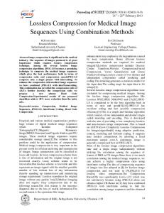
Figure 1: MLP prediction neighborhood. Before MLP processes its last level, the values of the pixels with circles in them are known. The pixels with numbers in their circles are used to predict the value of the pixel at the center, marked with a square. The numbers in the circles are the relative weights given to the predicting pixels; if all 16 points can be used for prediction, the prediction will be the weighted sum of the predicting pixels divided by 256. All unmarked pixels will also be predicted during the last level. The last level of the process is illustrated in Figure 1. The best predictions come from linear combinations of the nearest 4, 12, or 16 pixels, the coecients being chosen to perform polynomial interpolation. Prediction using 16 pixels is shown in Figure 1; the coecients are those which exactly t a polynomial of the form 3 X 3 X

i=0 j =0

aij xi y j

to 16 data points arranged as in the gure. In passing, we note that the predicting pixels are symmetrically placed, and have only three dierent weights, namely w1 = 81, w2 = ,9, and w3 = 1. Since the weights are normalized, dierent prediction methods dier only in the ratios r21 = w2=w1 and r32 = w3=w2; in this case the ratios are the same: r = r21 = r32 = ,1=9. In practice, we can obtain slightly better compression for many images by using dierent predictors for dierent levels. Using r = 0 for all but the last two levels (giving 4point prediction), r = ,0:06 for the next-to-last level, and r = ,0:12 for the last level improves compression for most of our test images by about one half percent. Note also that the corner pixels have very low weights and hardly contribute to the prediction, so we can safely omit them. These corrections are somewhat ad hoc and do not give a large improvement, so do not include them in our experimental results. Arithmetic coding can encode the prediction errors optimally with respect to any

2 MODELING BY VARIABILITY INDEX

3

given error model. Finding a good model is at least as important for compression eciency as making good predictions. Using too at a distribution gives too low a probability (and hence an excessively long code) to small error values, which occur frequently. On the other hand, using too peaked a distribution allocates too little probability to large errors. To keep the code length short, we prefer that the error modeling be done implicitly, with no need to transmit side information about the models used. Of course, the decoder must be able to mirror any error-modeling computations performed by the encoder. In this paper we introduce the notion of error modeling by variability index. In Section 2 we present and motivate the algorithm. In Section 3 we use the variability index as an experimental tool to show that prediction errors are not always Laplace distributed, as is widely assumed. We also indicate a family of distributions that can provide more accurate error models. In Section 4 we describe experiments showing that application of the variability index algorithm to Laplace distributions leads to an improvement in compression eciency of about 4 percent compared with implementations with explicit transmission of variances; further re nement by allowing a wider family of error distributions gives another half percent improvement. In Section 5 we discuss the direction of our current work.

2 Modeling by Variability Index In this section we assume that prediction errors are random variates from a Laplace (or symmetric exponential) distribution with zero mean. This assumption is based on considerable experimental evidence beginning with O'Neal [6], although in Section 3 we provide evidence that Laplace distributions are not always the best models for predictive coders. Our goal is to estimate the local variance of the pixel prediction errors in a given level of the MLP encoding. This will allow us to select the appropriate Laplace distribution (the one with the estimated variance) to use in encoding each pixel's prediction error by arithmetic coding. Using a single variance for the entire level (as in [2]) disregards local variations in the image; estimating and explicitly encoding variances for small sections of the image (also done in [2]) incurs considerable overhead. It would seem that previously encountered prediction errors of nearby pixels would be related to a given pixel's error, but there is no obvious way to use them directly. We estimate the variance by an indirect method: for each pixel we compute a variability index, a quantity strongly correlated with the local variance. On the supposition that pixels with similar variability index will have similar error models, we adaptively estimate the local variance based on the variability index. The algorithm is as follows: 1. For each pixel in the current level, we compute the variability index. 2. We sort the pixels in variability index order. 3. We initialize the variance estimate V . The choice of the initial value of V is not

3 DISTRIBUTION SELECTION

4

critical|for convenience we use the value it had one tenth of the way through the previous level. 4. For each pixel (in order of decreasing variability index): (a) We code the prediction error d, using a distribution with zero as its mean and V as its variance. (b) We use the prediction error d to update V . The variance is just the mean squared error; our variance estimate is a weighted mean squared error, computed by exponential smoothing: V := f V + (1 , f ) d 2 ; where f is a smoothing parameter. Since the prediction error d is coded in step 4(a), both the encoder and the decoder can use its value in step 4(b). Note that the variability index is used only for sorting the pixels, then discarded. We use decreasing variability index order because compression eciency is less dependent on accurate variance estimates for large variances; hence we encode pixels with large variances rst in each level, before our variance estimate has stabilized. The sorting step removes any natural ordering of the pixels, so both the encoder and the decoder must maintain the pixel coordinates. We have tried several dierent quantities for the variability index, including both intensity values and prediction errors of pixel neighborhoods of various sizes. Empirically, the most eective is simply the variance of the four nearest pixels. The smoothing parameter f must also be selected. Experiments show that the best results come from a large value like 0.992; smaller values make the estimated variance too sensitive to random uctuations in the variability index.

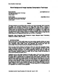
3 Distribution Selection When we code the pixels of a level in variability index order, we can plot histograms of the error distributions for dierent values of the variability index. A typical set of plots is shown in Figure 2. Two facts are apparent. First, the error distributions are not always Laplacian; in fact, for large variability index they appear closer to normal. Second, the distributions become closer to the Laplace distribution for smaller values of the variability index. This leads us to consider a family of generalized symmetric exponential distribution functions which includes both the Laplace distribution and the normal distribution. Distributions in this family have the form xn : (1) fn; (x) = n exp , n From the constraints on a probability distribution with variance 2, we can nd the values of parameters n and n: n ,(3=n) 1=2 ,(3 =n) n=2 n = ; n = : 2 ,(1=n)3 ,(1=n)

!

!

3 DISTRIBUTION SELECTION

5

Actual

Laplace

Normal Decreasing variability index ,! Figure 2: Histograms showing distributions of prediction errors. The top row shows the actual distributions of prediction errors for eight batches of 16,384 points each taken from the last level of MLP's coding of Band 4 of the Donaldsonville Thematic Mapper data set. The variability index decreases from left to right. The second and third rows show the discretized Laplace distributions and normal distributions with the same variances as the actual data in the corresponding column. The horizontal lines are at intervals of 10 percent probability; prediction errors from ,20 to +20 are plotted.

p

p

For the Laplace distribution (n = 1), we have p 1 = 1= 2 and 1 = 2; for the normal distribution (n = 2), we have 2 = 1= 2 and 2 = 1=2. We can use these distributions to optimize the exponent n in Equation (1), either image by image or for a class of images. The best values of n for our individual test images range from 1.0 to 1.9, the best overall value being 1.25. For many of our test images we obtain a further slight improvement when we vary the exponent within each level; in our experiments we use a given starting exponent and reduce it linearly toward 1 as we progress through each level. The improvement obtained by using a non-Laplace distribution is about a half percent; the extra improvement obtained by varying the exponent within a level is small, as is the improvement from selecting the optimal exponent image by image. It appears that the distributions we see are actually mixtures of normal or nearnormal distributions. High variability indices can arise only in regions with high local variance, so the mixture distribution contains contributions from only a small range of distributions. Low variability indices, on the other hand, can come either from regions with low local variance or from the not unusual occurrence of small deviates in regions with high local variance. The resulting mixture has contributions from many dierent distributions, and tends to be more peaked near zero; this gives the characteristic Laplace distribution shape.

4 COMPARATIVE RESULTS

6

4 Comparative Results Our experiments involved compressing 28 eight-bit grayscale images. We report our results both in terms of compression ratio (original size divided by compressed size) and in terms of a new measure called compression gain, described in Section 4.1. In Section 4.2 we brie y describe the test images and the compression methods compared, and we present the results in narrative, tabular and graphical form.

4.1 Compression gain

A robust measure of compression performance, called compression gain, is introduced in [2]. Here we give a slightly dierent formulation, using a more convenient scale. We de ne the compression gain by reference size ; (2) compression gain = 100 log e compressed size where the reference size and compressed size are expressed in the same units, usually either total bytes in the le or average bits per pixel. Compression gain is expressed in percent log ratio, denoted by the sign. Since loge (1 + x) x for small x, a dierence of any given small percent log ratio means almost the same thing as the same dierence expressed as an ordinary percentage. For the reference size we may choose the original le size, the zero-order entropy of the le, or the size of the compressed le produced by some standard lossless compression method. The logarithm in Equation (2) gives us additivity, so we can simply subtract the compression gains of two methods to nd the dierence between them, expressed in a percentage-like quantity. Coding eects, often expressed as percentages of code length, can be given as losses that can simply be subtracted from the compression gain of the modeling method. In this form we can clearly separate coding and modeling, and we can see how tiny the coding eects are. The gain/loss terminology is natural: larger numbers mean better compression.

4.2 Test procedures and results

The 28 images comprising our test data include 21 Landsat Thematic Mapper images and seven other images (the \USC images") widely used in compression studies. There are three Landsat data sets, each consisting of seven images (spectral bands); the locations are Washington, D.C., Donaldsonville, Louisiana (90 kilometers west of New Orleans), and Ridgely, Maryland (70 kilometers southeast of Baltimore). Each band is coded independently of the other bands; we do not attempt to make use of the correlation between bands in a data set. All images consist of 512 512 8-bit grayscale pixels except the Ridgely images, which are 368 468 pixels. Each of the Landsat data sets contains one highly compressible image (compressible to better than 8 : 1) and six \normal" images. In Table 1 we report compression ratios for all 28 images using a number of compression methods, including three versions of the MLP algorithm. The same results


7

are presented as compression gains in Table 2, and in graphical form in Figure 3. To avoid cluttering the graphs in Figure 3 we include results for only one version of MLP, and to keep the scale large we omit data for the three highly compressible Landsat images. The CCITT/ISO Joint Photographic Experts Group (JPEG) has recently proposed a standard for image compression [1] that addresses both lossless and lossy compression. We compare our results with the lossless mode of the JPEG proposed standard. The JPEG lossless mode is based on prediction by one, two, or three points, followed by Human coding or arithmetic coding; encoding proceeds in raster scan order. The standard gives some latitude to implementors; we report results from an implementation based on two-point prediction with arithmetic coding. For all except the three highly compressible Landsat images, two-point prediction provides 4 to 10 more compression gain than three-point prediction. We also include results for the Minimax coder, AT&T's original lossless compression submission to the JPEG, and for the Unix compress program. Figures for the Minimax coder are available only for the Landsat images, not the USC images. We report results for three versions of the MLP algorithm. The rst is the original MLP algorithm, with limited error modeling: we assume Laplace distributions and compute and transmit a single variance for each level. The second also uses Laplace distributions, and estimates variances using the variability index technique, with scaling factor f = 0:992. In the third we use Equation (1) with n starting at 1:5 in each level, falling to n = 1 (Laplace) by the end of each level. This is the method included in Figure 3. As noted in Section 2, there is only a small improvement when we optimize n for each image or vary the exponent within each level. Optimizing for each image requires compressing each image many times, so we omit that step in our reported results; varying the exponent within each level is a simple procedure that does improve compression slightly, so we include that step. Here we summarize the methods tested together with the abbreviations used in Tables 1 and 2 and Figure 3. Abbreviation JPEG Original

Compression Method JPEG lossless mode, with two-point prediction Our MLP method, using Laplace distributions and a single variance for each level n=1 Our MLP method, using Laplace distributions and variance estimation by variability index n = 1:5 to 1 (MLP{VI) Our MLP method using the variability index, with the exponent varying from 1.5 to 1.0 in each level MM coder AT&T Minimax coder, with two-point prediction compress Unix compress program In our experiments we nd that using MLP with the variability index technique gives the best compression for all images; it is about 7 percent better than JPEG


Image

8

Multi-level Progressive (MLP) Index JPEG Original n Variability = 1 n = 1:5 to 1 MM compress

W1 W2 W3 W4 W5 W6 W7 D1 D2 D3 D4 D5 D6 D7 R1 R2 R3 R4 R5 R6 R7 Landsat average

2.07 2.67 2.28 1.81 1.68 7.92 2.10 2.26 3.07 2.58 1.85 1.82 9.25 2.17 2.28 2.94 2.45 2.24 1.78 2.08 7.43 2.41

2.16 2.74 2.37 1.90 1.76 8.66 2.20 2.27 2.92 2.45 1.89 1.83 9.61 2.21 2.40 3.04 2.55 2.32 1.85 2.17 8.06 2.48

2.20 2.82 2.43 1.92 1.78 9.65 2.22 2.40 3.23 2.72 1.97 1.94 11.14 2.30 2.44 3.14 2.64 2.41 1.93 2.23 8.70 2.58

2.21 2.83 2.44 1.93 1.80 9.74 2.23 2.41 3.24 2.72 1.98 1.95 11.25 2.31 2.46 3.17 2.66 2.42 1.94 2.25 8.76 2.59

couple crowd lax lena man woman1 woman2 USC average

1.54 1.87 1.31 1.72 1.64 1.58 2.28 1.66

1.57 1.79 1.34 1.80 1.64 1.58 2.38 1.68

1.64 2.03 1.38 1.89 1.75 1.67 2.51 1.78

1.64 2.03 1.38 1.89 1.75 1.67 2.50 1.78

2.15 2.76 2.36 1.88 1.74 8.08 2.17 2.34 3.16 2.65 1.91 1.87 9.35 2.23 2.38 3.07 2.56 2.33 1.85 2.15 7.85 2.50

1.70 2.21 1.92 1.46 1.34 5.36 1.70 1.79 2.36 1.99 1.34 1.34 6.14 1.65 1.79 2.26 1.86 1.76 1.34 1.58 5.50 1.87 1.17 1.31 1.04 1.14 1.15 1.30 1.40 1.20

Table 1: Compression ratios (original le size divided by compressed le size) for 28 grayscale images. Figures for the Minimax coder are not available for the USC images.


Image

9

Multi-level Progressive (MLP) Index JPEG Original n Variability = 1 n = 1:5 to 1 MM compress

W1 W2 W3 W4 W5 W6 W7 D1 D2 D3 D4 D5 D6 D7 R1 R2 R3 R4 R5 R6 R7 Landsat average

| | | | | | | | | | | | | | | | | | | | | |

4.0 2.4 3.6 4.6 4.9 8.9 4.6 0.2 ,5:0 ,5:3 2.4 0.5 3.9 1.8 5.1 3.6 3.9 3.7 3.7 4.4 8.2 2.6

5.9 5.4 6.2 6.0 6.1 19.8 5.8 6.0 5.0 5.2 6.5 6.4 18.6 5.9 6.7 6.9 7.2 7.4 7.6 7.1 15.8 6.7

6.3 5.8 6.6 6.7 6.7 20.7 6.3 6.4 5.2 5.4 7.1 6.8 19.6 6.5 7.6 7.8 8.1 8.0 8.3 8.0 16.5 7.3

couple crowd lax lena man woman1 woman2 USC average

| | | | | | | |

2.0 ,4:3 2.0 4.3 0.0 ,0:1 4.2 1.1

5.9 8.4 5.1 9.3 6.7 5.6 9.3 7.0

6.3 8.3 5.3 9.4 6.7 5.5 9.2 7.0

3.6 3.4 3.5 4.0 3.6 2.0 3.5 3.2 2.8 2.7 3.2 2.8 1.1 2.7 4.5 4.4 4.1 4.1 3.7 3.7 5.5 3.4

,19:9 ,18:9 ,17:2 ,21:6 ,22:6 ,39:1 ,21:2 ,23:5 ,26:6 ,26:1 ,32:1 ,30:6 ,41:0 ,27:3 ,24:3 ,26:0 ,27:7 ,23:8 ,28:3 ,27:3 ,30:1 ,25:3

,27:4 ,35:4 ,23:5 ,41:8 ,35:2 ,19:2 ,48:8 ,32:3

Table 2: Compression gains for 28 grayscale images, expressed in percent log ratio ( ) using JPEG lossless mode compression as the reference value. Figures for the Minimax coder are not available for the USC images.


(a)

3:1

Compression Ratio

10

MLP{VI MM coder JPEG

2:1

compress

1:1

D2 W2 R3 W3 D1 R6 W1 D5 W4 wo2 len wo1 lax R2 D3 R1 R4 D7 W7 D4 R5 W5 cro man cou

Landsat Thematic Mapper images

(b)

+10

USC images

MLP{VI

Compression Gain +5 JPEG

MM coder R5 R6 R2 D4 W4 W3 D1 W1 D3 len cro cou lax R3 R4 R1 D5 W5 D7 W7 W2 D2 wo2 man wo1

Landsat Thematic Mapper images

USC images

Figure 3: (a) Compression ratios (original size divided by compressed size) arranged in order of decreasing compressibility, measured by the compression ratio using MLP{ VI. (b) Compression gains measured with respect to JPEG lossless mode, expressed in percent log ratio ( ) and arranged in order of decreasing compressibility as measured by the compression gain using MLP{VI. Landsat images are identi ed by data set and band number. Images D6, W6, and R7 are not included: they are all highly compressible, and would appear o the scale in both graphs. The USC images are identi ed by the rst three letters (or rst two letters and last digit) of their names. Figures for the Minimax coder are not available for the USC images.

5 CONCLUSIONS

11

lossless mode and almost 4 percent better than the Minimax coder. The variability index technique improves on the original MLP algorithm by over 4 percent, and using a dierent exponent in Equation (1) gives another half percent compression, at least for the Landsat images. Figures for the compress command are included only to show how poorly suited it is for image compression. As we have noted, the MLP method runs slowly. The prediction step, the computation of the variability index, and arithmetic coding all make heavy use of the processor. However, hardware continues to become faster and cheaper. A typical run of the MLP program takes about 2 minutes and 26 seconds on a Sun SPARCstation 1, the equipment with which we began this research; now we can run it in about 43 seconds on a SPARCstation 10, an improvement factor of 3.4. It really does make sense to try for maximum compression; the hardware will catch up!

5 Conclusions We conclude that using the variability index for the error modeling component of the MLP algorithm is extremely eective. It gives good estimates of local pixel variances without requiring any overhead (side information) to describe the models. In addition, the use of the variability index to classify pixels according to their local variability allows us to see that prediction errors are best modeled by a Laplace distribution only for groups of pixels with low variability; this leads us in turn to the use of dierent distributions. Since the original MLP algorithm gives results generally better than the JPEG lossless mode and comparable to the AT&T Minimax coder, and the variability index technique gives more than 4 percent better compression than the original method, we see that the variability index technique improves substantially on other available lossless image compression methods. It also retains MLP's advantages of progressivity and parallelizability. We are currently investigating several questions. We wish to nd a theoretical basis for the variability index; we expect that this will enable us to estimate the variance directly from the variability index, without the sorting step and the indirect adaptive estimation. We are also investigating the choice of exponent in Equation (1); an understanding of the factors that combine to produce the optimal exponent at a given pixel will enable us to estimate the exponent directly, leading to still better compression. A related issue is to determine the distribution mixing process that leads to the observed error distributions. In other recent work [3,5], we identify simpli cations that enable us to obtain maximum speed at some cost in compression eciency. The resulting non-progressive compression system (called FELICS) gives compression about 7 worse than MLP and about the same as the JPEG lossless mode. FELICS runs nearly 50 times faster than MLP, ve times faster than a commonly used implementation of the JPEG lossless mode, and as fast as the Unix compress program. We have also investigated a progressive version of FELICS [4] that uses MLP's pixel sequence; it obtains about 1 better compression than non-progressive FELICS at the cost of a small decrease in speed.

5 CONCLUSIONS

12

Acknowledgments. We wish to thank James C. Tilton of the NASA Goddard

Space Flight Center for supplying the images used for our experiments. We also wish to thank Allan R. Moser of E. I. duPont de Nemours and Company (Inc.) for assisting us with experimental evaluation of lossless mode JPEG compression.

References [1] \Digital Compression and Coding of Continuous-Tone Still Images, Part 1, Requirements and Guidelines," ISO/IEC JTC1 Draft International Standard 10918{ 1, Feb. 1991. [2] P. G. Howard & J. S. Vitter, \New Methods for Lossless Image Compression Using Arithmetic Coding," Information Processing and Management 28 (1992), 765{779. [3] P. G. Howard & J. S. Vitter, \Design and Analysis of Fast Text Compression Based on Quasi-Arithmetic Coding," Information Processing and Management 30 (1994), 777{794, also appears in shorter form in the proceedings of the Data Compression Conference, J. A. Storer and M. Cohn, eds., Snowbird, Utah, March 30-April 1, 1993, 98-107. [4] P. G. Howard & J. S. Vitter, \Fast Progressive Lossless Image Compression," in Image and Video Compression Conference, Symposium on Electronic Imaging: Science & Technology #SPIE{2186, San Jose, California, Feb. 9-10, 1994, 98{109. [5] P. G. Howard & J. S. Vitter, \Arithmetic Coding for Data Compression," Proc. IEEE 82 (June 1994), 857{865. [6] J. B. O'Neal, \Predictive Quantizing Dierential Pulse Code Modulation for the Transmission of Television Signals," Bell Syst. Tech. J. 45 (May{June 1966), 689{ 721.