Estimating Sampling Errors in Large-Scale Temperature Averages

2548

JOURNAL OF CLIMATE

VOLUME 10

Estimating Sampling Errors in Large-Scale Temperature Averages P. D. JONES, T. J. OSBORN,

AND

K. R. BRIFFA

Climatic Research Unit, School of Environmental Sciences, University of East Anglia, Norwich, United Kingdom (Manuscript received 23 May 1996, in final form 27 January 1997) ABSTRACT A method is developed for estimating the uncertainty (standard error) of observed regional, hemispheric, and global-mean surface temperature series due to incomplete spatial sampling. Standard errors estimated at the grid-box level [SE2 5 S 2(1 2 r¯)/(1 1 (n 2 1)r¯)] depend upon three parameters: the number of site records (n) within each box, the average interrecord correlation (r¯) between these sites, and the temporal variability (S 2) of each grid-box temperature time series. For boxes without data (n 5 0), estimates are made using values of S 2 interpolated from neighboring grid boxes. Due to spatial correlation, large-scale standard errors in a regionalmean time series are not simply the average of the grid-box standard errors, but depend upon the effective number of independent sites (Neff) over the region. A number of assumptions must be made in estimating the various parameters, and these are tested with observational data and complementary results from multicentury control integrations of three coupled general circulation models (GCMs). The globally complete GCMs enable some assumptions to be tested in a situation where there are no missing data; comparison of parameters computed from the observed and model datasets are also useful for assessing the performance of GCMs. As most of the parameters are timescale dependent, the resulting errors are likewise timescale dependent and must be calculated for each timescale of interest. The length of the observed record enables uncertainties to be estimated on the interannual and interdecadal timescales, with the longer GCM runs providing inferences about longer timescales. For mean annual observed data on the interannual timescale, the 95% confidence interval for estimates of the global-mean surface temperature since 1951 is 60.128C. Prior to 1900, the confidence interval widens to 60.188C. Equivalent values on the decadal timescale are smaller: 60.108C (1951–95) and 60.168C (1851–1900).

1. Introduction This paper addresses the often asked question: ‘‘How accurate are the hemispheric and global-mean surface temperatures records?’’ A related question is: ‘‘How different must one January’s temperature, or one year’s temperature, be from another before the two can be considered significantly different?’’ It is clear that a greater difference is required for a difference to be significant between two Januarys than between two years. Lengthening the timescale, a smaller difference would be significant if two annual decadal averages were being compared. The question posed in the first sentence is therefore incomplete, as it does not specify the timescale. The issue is not confined to instrumental temperature records but has application in other areas such as hydrology, where the accuracy of mean catchment precipitation is an important issue. The issue is, therefore, common to sciences where averages of correlated time series are derived.

Corresponding author address: Dr. Philip D. Jones, Climatic Research Unit, School of Environmental Sciences, University of East Anglia, Norwich NR4 7TJ, United Kingdom. E-mail: [email protected]

q 1997 American Meteorological Society

The errors in large-scale temperature series discussed in this paper are just the errors due to sampling. The other group of errors relate to instrumental reading or coding mistakes and potential biases or inhomogeneities in station temperature time series. For regional temperature series, large mistakes will be discovered during quality control (e.g., outlier checks) while small mistakes should be random and any errors will cancel rapidly as the number of stations involved increases in size. Supporting this, Weber and Madden (1995) use optimal averaging techniques (Gandin 1963) to estimate sampling errors and show that if realistic measurement errors (e.g., after Trenberth et al. 1992) are included, the value of the optimal average does not substantially change. Biases or inhomogeneities can lead to systematic errors (e.g., due to urbanization effects at land stations and the bucket/intake problem with sea surface temperatures). It is assumed here that these have been adequately dealt with in the station by station homogeneity assessment (see Jones 1994; Folland and Parker 1995, and references therein for details). In a related study, Smith et al. (1994) refer to these errors as data errors and assume that they are uncorrelated with each other. Some of the issues have been addressed before. The extent to which the more sparsely available nineteenth

OCTOBER 1997

JONES ET AL.

century instrumental networks monitored large-scale temperatures has been assessed using ‘‘frozen grids’’ by Jones et al. (1986a,b) and Parker et al. (1994), and using globally complete fields from the microwave sounding unit data (Spencer and Christy 1992b) by Karl et al. (1994). The same question has been investigated using model-derived grids that, because they are complete, can assist in assessing the effects of regions always missing from analyses (Trenberth et al. 1992; Madden et al. 1993; Karl et al. 1994). Although the terminology may be different, the same issues are explored in optimal interpolation or averaging by Gandin (1963), Kagan (1979), Hardin and Upson (1993), Smith et al. (1994), Shen et al. (1994), and Weber and Madden (1995), and with kriging techniques by Gunst (1995). [Cressie (1991, 106), for example, states that optimal averaging, interpolation, and kriging are essentially the same, having been developed in meteorology and geology simultaneously.] The Karl et al. (1994) study specifically addresses the effect of spatial sampling errors on the estimates of trends in regional temperature series, concluding that the error of estimation of the global-mean trend over the last 100 yr is an order of magnitude smaller than the trend [;0.58C(100 yr)21] itself. The spatial structure of the sampling error and its temporal changes is also a necessary requirement for a complete analysis of the climate change detection problem (see, e.g., Hegerl et al. 1996). Previous work has considered the issue without regard for timescale. Smith et al. (1994), for example, calculate standard errors for various regional temperature time series on seasonal and annual interannual timescales and plot the series after application of a 5-yr binomial filter for clarity. As will be shown in this paper, errors on a 5-yr timescale are smaller. There seems to be no shortcut to transferring errors from one timescale to another: errors should be calculated over the timescale of interest or the timescale on which they are to be displayed. This paper attempts to bring the previous work and the timescales together. The key parameter in this and some earlier studies is the effective number of independent samples (Neff) over the domain (region) or globe. Madden et al. (1993) refer to this as the ‘‘spatial degrees of freedom.’’ Once the significance of this concept is grasped and that this effective number reduces with increasing timescale, the more difficult problem of estimating Neff can be addressed. Both instrumental and coupled ocean–atmosphere general circulation model (GCM) control run data will be used to estimate Neff and the relationship between Neff and timescale. Depending on one’s viewpoint, the model data can be considered as providing support for the instrumental data or as a useful exercise in model validation. The paper has important implications for monitoring global temperatures, not the least of which is that the number of sites required to achieve a certain level of

2549

reliability depends on timescale. Both the methodology and the techniques can be applied to the regional and global average estimation of other variables in climatology. The paper is structured as follows. Section 2 discusses surface temperature data sources, both observed and modeled. Section 3 addresses the estimation of standard errors at the grid-box level. Section 4 considers these standard errors on the regional-to-global scale, given the spatial correlation inherent in the data, and addresses methods to estimate Neff. In section 5 the results of sections 3 and 4 are applied to instrumental and GCM temperature data and standard errors on different timescales are assessed. Section 6 summarizes the main conclusions. 2. Surface temperature data sources Two versions of observational grid-box temperature anomaly time series are used. The first is on a 58 3 58 grid-box network and is composed of surface air temperature (SAT) anomalies, referenced to the 1950–79 mean, from land stations combined with sea surface temperature (SST) anomalies, also from the 1950–79 mean, over oceanic areas. The construction of this dataset is described in Jones et al. (1991) and Jones and Briffa (1992). In this dataset (hereafter JB), both the constituent datasets (SAT and SST) were available on a 58 3 58 box grid. They were merged by taking the average of the two analyses where temperature anomalies existed from both SAT and SST. This occurred around coastlines and islands. The second dataset, referred to as IPCC, is a merger of the Jones (1994) SAT anomalies, with respect to 1961–90, with SST anomalies (from in situ measurements only) in the U.K. marine data bank (MOHSST6), also with respect to 1961–90 (Nicholls et al. 1996). MOHSST6 uses an underlying SST field for 1961–90 at 18 resolution. The 58 3 58 box value in anomaly terms is the average of at least one of the 25 constituent 18 box anomaly values. These two constituent datasets (SAT and SST) were combined using the algorithm developed by Parker et al. (1994). The land–ocean fraction was used for coastline boxes, but key ocean island SAT anomalies were given at least a weight of 0.25 (and, similarly, small coastal sea patches were given a minimum weighting of 0.25). In data-sparse ocean regions, an island with SAT data is likely to produce a more reliable estimate of the temperature anomaly than one from a few SST values in the surrounding ocean. Both observational datasets make use of SST anomalies over the ocean as a surrogate for air temperature anomalies. It has been shown by a number of authors, most recently by Parker et al. (1994), that the number of SST values in a 58 3 58 box is likely to be higher than for ship-based air temperatures (at least twice as high, if ship daytime air temperatures are ignored because of solar heating of decks). Furthermore, Trenberth

2550

JOURNAL OF CLIMATE

et al. (1992) and Parker et al. (1994) have implicitly shown that sampling errors are smaller for SST than ship-based air temperatures. Thus, even if the number of observations in a 58 3 58 box were the same, the SST anomaly value should have a smaller error at the grid-box level. Both observational datasets only extend back to the midnineteenth century. They have changes in spatial coverage through time, and both have regions (such as the mid-to-high latitudes of the southern oceans) always missing. For these reasons, we also make use of surface air temperature fields derived from the control runs of three GCMs. These are the 1000-yr control run of the Geophysical Fluid Dynamics Laboratory (GFDL) model (Stouffer et al. 1994), the 1000-yr control run of the latest Hadley Centre (HC) model (HadCM2; Mitchell et al. 1995), and the last 800 yr of the 1260-yr control run of the Max-Planck-Institut fu¨r Meteorologie (MPI) model (ECHAM1/LSG; von Storch 1994). Long GCM control runs provide complete data fields and have been used before to assess the importance of missing regions in large-scale temperature averages (Hansen and Lebedeff 1987; Madden et al. 1993). How well the GCM reproduces reality in a region with little data must be an open question, however. If the model does well in other regions, then it must be reasonable to place some faith in the variability it reproduces over the missing regions. In some respects, therefore, using models to assess error estimates could reasonably be viewed as a form of model validation. The longer GCM data are used to assess the changes to error estimates when considering large-scale and hemispheric averages on timescales longer than interannual (such as decadal and century). This is not possible using the instrumental data alone. The ability of models to produce realistic levels of variability on different timescales is an important issue in anthropogenic climate change detection (Santer et al. 1995). One of our only means of assessing how unusual the last 50 yr have been is to use model-generated estimates of natural variability. Such model estimates do not include external forcing variability from solar output changes nor changes in explosive volcanic frequency. They also have to be flux adjusted (e.g., Sausen et al. 1988) to avoid excessive model drift, and there is some controversy over the effect of these adjustments on apparent long timescale variability (Kerr 1994; Nakamura et al. 1994). Paleoclimatic data have the potential to quantify ‘‘real’’ natural variability on these timescales and some initial comparisons between these and long GCM-run temperatures suggest that model variability may be underestimated (Barnett et al. 1996). The situation may be worse as most paleoclimatic series tend to lose variability in the reconstruction, the longer the timescale (see, e.g., Briffa et al. 1996; Cook 1995). This does not preclude us from using the long GCM control runs to assist in these estimations; however, we must be very careful in the conclusions we draw.

VOLUME 10

It could be argued that any results derived from the observed data might be biased by the long-term warming that has occurred this century. To assess this, we compare the control simulation of the HC model with a perturbed simulation, also of the HC model. The perturbed simulation was forced with estimates of past greenhouse gas and sulfate aerosol concentrations from 1860 to 1990 (Mitchell et al. 1995). We also remove an estimate of the long-term warming signal (Wigley et al. 1997) from the observations and compare these results with the GCM control runs. 3. Error estimation We begin by considering the error at an individual 58 3 58 grid box. This error will be dependent on the number of individual stations or SST anomaly values within the box. The error will not be solely dependent on the number of observations, but also on the interannual variability of climate in the box. One station in a maritime region such as Ireland will have a smaller standard error than a single station value in a continental climate region such as Siberia. This is because in Siberia the spatial and interannual variability of air temperature is considerably higher. Kagan (1966; see Yevjevich 1972 for an English version), in both a theoretical and empirical study, found that the relationship between single-site precipitation standard deviations (si) and the standard deviation (Sˆ) of a multisite mean (of n sites) depended on the average intersite correlation (r¯); thus,

[

]

1 1 (n 2 1)r¯ Sˆ 2 5 s i2 n

(n $ 1).

(1)

The true areal standard deviation (S) can only be obtained from an infinitely sampled catchment, although if r¯ is close to 1 (as is the case for annual-mean temperature on a 58 grid), then Sˆ is almost equal to S even for small n. Assuming that we have estimates of s2i and r¯ that are unbiased, we can in fact obtain S 2 by letting n → ` in Eq. (1), which becomes S 2 5 s2i r¯.

(2)

Although Eq. (1) is undefined for n 5 0 (the average of zero sites has no standard deviation defined), Eq. (2) is simply a relationship between the statistics of points in a box and the variance of the true areal variance for the box. It is independent of the number of site records in a grid box. To obtain accurate estimates of singlesite variance and intersite correlation does, of course, require there to be some sites in the box, and a higher density of sites will probably lead to better estimates. We use Eq. (2) even when n 5 0, with s2i and r¯ estimated by interpolation from the statistics of neighboring boxes where estimates can be made. In a later study (Wigley et al. 1984; see also Briffa

OCTOBER 1997

JONES ET AL.

and Jones 1990), the standard error (SE) of estimation of the areal precipitation series was related to the standard deviation of the areal series (S); thus, SE 2 5 S 2

[

]

1 2 r¯ . 1 1 (n 2 1)r¯

(3)

This implies that SE2 5 S 2 if r¯ 5 0 or n 5 0, but that the error decreases (SE2 , S 2) as the common variance increases (r¯ . 0). The error decreases hyperbolically as the number of stations increases (i.e., more rapidly for low n). Combination of Eqs. (2) and (3) yields SE 2 5

s i2 r¯ (1 2 r¯) . 1 1 (n 2 1)r¯

(4)

The limiting cases of the above equation are for n 5 0, SE2 5 s2i r¯ and for n 5 `, SE2 5 0. An alternative to the above might assume S 5 Sˆ in Eq. (3), combining the result with Eq. (1) (for n . 0 only, as the latter is undefined for n 5 0), to produce

1

2

1 2 r¯ d SE 2 5 s i2 , n

(5)

with the ˆimplying that this standard error is an estimate of the true value defined in Eq. (4). Ratioing the last two equations shows that Eq. (5) would always give larger (i.e., more conservative) values than does Eq. (4): d SE 2 1 1 (n 2 1)r¯ 5 $ 1. SE 2 nr¯

(6)

The difference is generally small for temperature data (see section 3e) as our estimates of r¯ are generally in the range 0.7–0.95. In the rest of this paper we use Eq. (4), but give an example of how the estimated standard errors would increase by using Eq. (5). Application of the above to the grid-box temperature data requires estimation of the station standard deviations s2i , r¯, and a value for n. The value of n over land areas is clearly the number of stations, but over ocean areas the number of SST observations is not the same quantity. We address this issue and how to estimate s2i (and hence S 2) and r¯ next. a. Estimation of s2i We consider the analysis of the observed datasets first. For the land areas, s2i could be estimated from the stations available in a given month, preferably calculated over a common period such as the reference period associated with the grid-box temperature dataset (e.g., 1961–90 for Jones 1994). Such a calculation is problematic, however, because station availability is rarely constant and because a number of stations have only estimated averages for 1961–90. It would seem preferable, therefore, to estimate s 2i for each box from the variance (Sˆ 2) of the gridded temperature time series. This ignores differences caused

2551

by varying station density and location of available stations through time (although the latter is ameliorated by the fact that there are likely to be only small variations between individual site si values, the differences being due primarily to orography and the distance from any coast). We do not use the grid-box variance (Sˆ 2) as S2, since it is not computed from an infinitely sampled dataset. Instead we use Eq. (1) to estimate s2i as Sˆ2n/(1 1 (n 2 1)r¯), using an Sˆ 2 calculated for a modern reference period and the mean n during that period. Over ocean areas, the station concept is not appropriate. Here, estimation of s2i is only possible using a grid-box time series (i.e., the method we also use for the land areas) composed of individual measurements taken by various ships. The number of observations per box (m) is also inappropriate to use for n, as the measurements do not form a continuous series as for land stations. The SST compilations generally accept a gridbox value if there are at least three to five in situ observations in an individual month (Jones et al. 1991; Parker et al. 1994). As in situ observations are used, there is no need to consider day–night differences in SSTs that occur with skin temperatures from satellites (Reynolds 1988). We estimate the effective number of station time series in an ocean box by dividing the number of SST observations in a box (m) by 5, ensuring that n is greater than or equal to 1. We have also used divisors of 3 and 10, and find differences of no more than 1% for the standard error of the global mean temperature time series. For both ocean and land areas, Sˆ 2 has been estimated on the interannual timescale from the grid-box series using the 1951–80 time period. In this estimation, n is taken as the average number of stations available over the 30 yr for land regions and the average number of SST observations divided by 5 (i.e., 0.2 m) for oceanic areas. We use 1951–80 because it is the period of best data coverage and because a longer period, or the 1961– 90 period, might inflate Sˆ 2 (and hence s2i ) due to stronger long-term warming signals. For the interdecadal timescale, the grid-box mean and characteristic station standard deviations are computed similarly, but using the longer 1901–90 period. For the GCM data, s2i values are also estimated from the variances of the grid-box means, but by the application of Eq. (2), since we assume that these are true areal variances (i.e., S 2) computed from the effectively infinitely sampled (i.e., n 5 `) grid-box mean temperatures that the GCMs produce. b. Estimation of r¯ For boxes with many stations, r¯ could be estimated from the station data. This procedure does not produce reliable values when few station records exist. It is not possible for land boxes with only one station present or any marine boxes. [Over half the boxes in the Jones (1994) dataset have less than three stations per box (see

2552

JOURNAL OF CLIMATE

VOLUME 10

Jones 1995).] It may also be biased by nonuniform distribution of stations within a box. To estimate r¯, therefore, we make use of related studies of temperature correlation decay lengths (Briffa and Jones 1993; Jones and Briffa 1996). In these papers, grid-box temperature anomaly values have been used to derive correlation decay lengths of the form r 5 e2x/x0,

(7)

where r is the correlation between neighboring boxes, x is the distance between the box centers, and x0 is the characteristic correlation decay length. This correlation function [Eq. (7)] is positive definite on a sphere (Yaglom 1987). Values of x0 were estimated for each grid box using seasonal- and annual-mean data in Briffa and Jones (1993) and for decadal averages in Jones and Briffa (1996). In both studies only grid boxes within 6208 of latitude and 6458 of longitude of the grid box were used in the estimation of x0. Alternative functional forms using Bessel functions have been used by Vinnikov et al. (1990; see also Madden et al. 1993), based on earlier theoretical work by Kagan (1979). The x0 values calculated in this exercise enable us to estimate r¯ within an individual grid box by integrating Eq. (7) up to a distance X (the distance between opposite corners of a grid box; X being slightly greater for an equatorial than a polar box). For an individual box, X is the maximum possible distance between stations within a box: Xr¯ 5

E

X

e 2x/x0 dx,

(8)

0

giving r¯ 5

1

2

x0 1 2 e 2X/x0 . X

(9)

Use of the correlation decay length between grid-box averages (x0) for estimating correlations between stations can be shown to be valid (results not shown). c. Isotropic results Briffa and Jones (1993) and Jones and Briffa (1996) fitted Eq. (7) by taking the logarithm of the r values and using linear regression. Although both studies clearly state they omitted points when r # 0, what effect does this have on the results? This method is compared (in appendix A) with an alternative method that fits Eq. (7) iteratively to the data until the root-mean-squared error is minimized. The latter method allows all r values to be retained and does not require the taking of logarithms; this is the approach used for the remainder of this study. A related issue is that estimation based on Eq. (7) assumes an isotropic reduction in the correlation with distance. In appendix B we examine this by expanding Eq. (7) to allow for anisotropy and find that

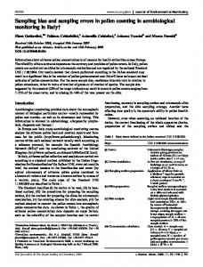
FIG. 1. Zonally averaged correlation decay lengths (km) computed from annual means of the JB (dotted line) and IPCC (dashed line) datasets, using the method of Briffa and Jones (1993) to fit the decay functions. Also shown are the results of using the new method of fitting the decay functions, applied to the IPCC dataset (continuous line).

the isotropic assumption is valid in some instances. We also find, however, that the calculation of r¯ and Neff (see section 4a) is likely to result in similar values whether an isotropic or an anisotropic function is used. The isotropic function [Eq. (7)] is, therefore, used for the remainder of this study. All model and observational (JB and IPCC) results have been computed using the isotropic function [Eq. (7)] fitted directly to the full, untransformed set of (correlation, distance) data pairs. Using the IPCC dataset (Briffa and Jones 1993 used the JB dataset) led to a considerable reduction in low and midlatitude correlation decay lengths (Fig. 1; cf. dashed and dotted lines). The possible reason for this is that the JB dataset was originally constructed over land on a 58 lat 3 108 long gridpoint basis and was reduced onto the 58 3 58 grid size used here using an algorithm developed by Parker et al. (1994). Over continental areas, one 58 3 108 grid point effectively became two 58 3 58 grid boxes. This resampling may have led to an excessive correlation between pairs of grid boxes, as these were originally the same grid point, and hence to an inflated estimate of x0. The new method of fitting the exponential functions (retain r # 0, fit nonlinearly without taking logarithms) was applied to the IPCC dataset [Fig. 1; thick continuous line compared with the dashed line that used the method of Briffa and Jones (1993) for fitting the decay functions]. As expected from the tests described in appendix A, a further reduction was obtained (particularly on either side of the equatorial maximum). These final results (using the IPCC dataset and the new fitting procedure) are used throughout the remainder of this paper. Figure 2 shows a comparison of the correlation decay lengths for annual data on the interannual timescale be-

OCTOBER 1997

JONES ET AL.

2553

and east-central Pacific Oceans (Fig. 2). This is weaker in the MPI and GFDL models than in the observations, but much too strong in the HC model [a bias also noted by Tett et al. (1997)]. Correlation decay lengths are generally lower in the extratropics and least in the highest latitudes (although observed data availability is poorer there). An exception to this is the region of higher values that occurs over the Southern Ocean, which is of a similar magnitude (in the zonal means of the observations and of the GFDL model) to the tropical values on the interdecadal timescale. (Note that some of the spikes that occur in the observed results near the high-latitude extremes are due to the few grid boxes with sufficient data being sited in locations of relatively low or high x0.) Poleward of about 308, all models exhibit similar decay lengths, with the lower values over land in the MPI model (the only dataset to exhibit a clear land–sea difference in the extratropics) leading to slightly lower zonal means. d. The influence of climate change signals

FIG. 2. Correlation decay lengths (1000 km) of annual-mean temperatures from (a) IPCC observed dataset, (b) HC control run, (c) GFDL control run, and (d) MPI control run. Contour interval is 1000 km, values ,1500 km are darkly shaded, and missing data are lightly shaded (here and in all other figures).

tween the new analysis of the observed IPCC data and the results using the three GCM control runs. Similar calculations on the seasonal and decadal timescales have been made but are shown only as zonal averages (Fig. 3). All analyses show tropical maxima on all timescales (Fig. 3), associated with high x0 over the central Indian

All three models exhibit lower midlatitude correlation decay lengths than in the observed data, with the difference being greater (and extending to higher latitudes) the longer the timescale. Is this difference due to a systematic error in the models? If so, then it is an important result from a validation point of view, but it would also reduce our confidence in applying the model control integrations to the estimation of errors on longer timescales where the observed data is poorer or insufficient (decadal and century timescales). Another explanation for these differences is that the observations contain externally forced variability in addition to the natural internally generated variability, whereas the model control runs contain only internally generated variability. Although volcanic and solar forcings might be important, the enhanced radiative forcing due to the greenhouse effect is likely to be the largest external forcing in the observations. The response of the climate system to this forcing yields a global warming signal that will be present in the observations but absent in the model integrations with their fixed radiative forcing. If the signal pattern is highly spatially coherent, then it will tend to raise the correlation decay lengths when it is superimposed on the ‘‘natural’’ variability, thus explaining the differences between model and observations. The increase will be larger on the interdecadal timescale than on the interannual timescale, since the signal is stronger (relative to the noise), the longer the timescale. To test this possibility, two approaches have been followed. The first is to add the signal to one of the model control runs, which we do by making use of a perturbed, historically forced model integration carried out using the HC model (Mitchell et al. 1995). This has been forced with past estimates of greenhouse gas and sulfate aerosol concentrations, and the 130-yr equivalent to the 1880–1990 period has been analyzed in the same

2554

JOURNAL OF CLIMATE

VOLUME 10

FIG. 3. Zonally averaged correlation decay lengths (km) computed from IPCC observed dataset (thick continuous lines), HC control run (thin continuous lines), GFDL control run (dotted lines), and MPI control run (dashed lines) on the following timescales and seasons: (a) December– February (DJF), (b) March–May (MAM), (c) June–August (JJA), (d) September–November (SON), (e) annual, (f) decadal DJF, (g) decadal MAM, (h) decadal JJA, (i) decadal SON, and (j) decadal annual.

way as the model control integrations. The second approach is to subtract the signal from the observed record and analyze the residuals. The signal is not well known, however, and simply removing trends or applying a high-pass filter would also remove any natural century– timescale variability. Instead, a model-based estimate of the signal and its time evolution (described in detail in Wigley et al. 1997) is removed, and the residual data analyzed.

Results of these tests are given in Fig. 4 for the annual and decadal means. The observational and HC control run results are repeated for comparison, and it is clear that the global warming signal (either what we removed from the observations or added to the model by using the perturbed integration) is responsible for at least part of the differences between models and observations (cf. Figs. 3e and 3j for the other models). The historically forced HC model simulation (HC forced) produces

OCTOBER 1997

JONES ET AL.

2555

lengths (it is equivalent to adding the negative of the pattern). On the basis of these additional analyses, it appears that there is no significant difference between model results and observations in the Southern Hemisphere extratropics. In the Tropics, the GFDL and (to a lesser extent) the MPI models still underestimate interannual x0, but not interdecadal x0. The overestimate there by the HC model now appears even greater. In the Northern Hemisphere extratropics, interannual decay lengths are still slightly underestimated by all models. On the interdecadal timescale, the GFDL and HC models are poor between 208 and 508N, whereas the MPI model produces values that are too low throughout the hemisphere. Global average correlation decay lengths have been produced by a number of authors. Mann and Park (1993) quote 1500 km, presumably for monthly data although the timescale is not stated. Madden et al. (1993) found a value of 1200 km from a perpetual January GCM simulation. The global-mean x0 values found here are given in Table 1. They agree quite well with the earlier work, although considerably extending those analyses. e. Observed values of x0 and r¯

FIG. 4. Zonally averaged correlation decay lengths (km) computed from IPCC observed dataset (thick continuous lines), IPCC minus Wigley et al.’s (1997) climate change signal (thick dotted lines), Wigley et al.’s (1997) climate change signal alone (dashed line), HC control run (thin continuous lines), and HC historically forced perturbed run (thin dotted lines) for annual means on (a) annual and (b) decadal timescales.

greater correlation decay lengths than the control run did in the Southern Hemisphere (Fig. 4a), and the increase is larger on the interdecadal timescale (Fig. 4b). There is very little difference in the Northern Hemisphere, except for a slight increase in the high latitudes on the decadal timescale. The correlation decay lengths of the signal alone are very high (Fig. 4b), with an interhemispheric asymmetry due to the Northern Hemisphere response to smaller-scale sulfate aerosol forcing patterns. Once subtracted from the observations, the correlation decay lengths reduce. Once again, the difference is greatest in the Southern Hemisphere, and largest on the longer timescale (Fig. 4b). The fact that a reduction does occur increases our confidence that the model-derived signal is reasonable, since subtracting a coherent pattern that is not in the observations raises the correlation decay

On the interannual timescale, Briffa and Jones (1993) and this study find that observed values of x0 range from a minimum of about 750 km in the eastern North Pacific, to about 4500 km over the tropical parts of the Pacific and Indian Oceans. This characteristic distance is where the correlation with the central point falls to 1/e. Equation (9) gives r¯ values ranging from about 0.7 at 208– 408 of latitude over the Pacific Ocean and American continents to near 0.95 over the tropical Pacific and Indian Oceans. Extending this type of analysis to the decadal timescale gives an average observed x0 value for the globe of about 3700 km, compared to 2100 km on the interannual timescale. Additional global-mean values are given in Table 1. All r¯ values given there are computed using X [see Eq. (8)] for 58 3 58 grid boxes (see section 5 for details of the conversion from model grids to observed grid). Model r¯ values are lower than observed values, due in part to the influence of the global warming signal in the observed record on x0. We are now in a position to estimate standard errors for all boxes with data, by making estimates at each grid box of s2i and r¯ and knowing n. At this point it is possible to use Eqs. (4) and/or (5) to support a number of intuitive statements. For example, if a new station is being considered, it is best not only to locate it in a box without data, but also in one with a lower r¯ value. Searches for additional data are most valuable in regions with few stations per box and where r¯ is low. The above arguments explain why additional station data in interior parts of Asia, Africa, or South America would produce a greater reduction in standard errors than additional data in Europe or North America. Such arguments only hold during the twentieth century, as even in ‘‘data rich’’

2556

JOURNAL OF CLIMATE

VOLUME 10

TABLE 1. Variability and correlation parameters computed from observational and model datasets, for seasonal and annual results on interannual and interdecadal timescales. Values are given for global-mean grid-box temperature standard deviation (S¯ in 8C), global-mean correlation decay length (x0 in km), global-mean intragrid-box cross correlation (r¯), and the number of independent samples over the globe [Neff, estimated using Eqs. (14) and (15)]. Values in parentheses for Neff were estimated from Eq. (10). DJF S¯

x0

r¯

Neff

S¯

x0

r¯

Neff

MAM

JJA

SON

Annual

OBS HC GFDL MPI OBS* HC GFDL MPI OBS* HC GFDL MPI OBS HC GFDL MPI

0.74 0.87 0.98 0.73 1509 1699 1073 1053 0.77 0.78 0.72 0.71 37.6 (17) 30.1 (54) 72.5 (75) 75.2 (138) Decadal DJF

0.63 0.83 0.94 0.67 1490 1920 1059 1021 0.77 0.79 0.72 0.70 38.6 (12) 24.0 (34) 74.4 (62) 79.9 (146) Decadal MAM

0.56 0.81 0.83 0.56 1450 1767 1058 1067 0.77 0.78 0.72 0.71 40.6 (13) 28.0 (43) 74.5 (50) 73.3 (117) Decadal JJA

0.60 0.82 0.91 0.61 1505 1636 1071 1067 0.78 0.78 0.72 0.71 37.9 (14) 32.3 (43) 72.8 (58) 73.3 (123) Decadal SON

0.43 0.56 0.54 0.40 2093 2295 1364 1272 0.83 0.81 0.77 0.74 20.5 (7) 17.4 (20) 45.6 (27) 52.2 (83) Decadal

OBS HC GFDL MPI OBS* HC GFDL MPI OBS* HC GFDL MPI OBS HC GFDL MPI

0.30 0.31 0.33 0.26 2862 2152 1521 1383 0.83 0.82 0.78 0.75 11.9 (5) 19.5 (21) 37.1 (21) 44.4 (75)

0.28 0.29 0.34 0.24 3152 2350 1482 1328 0.84 0.82 0.78 0.74 10.2 (3) 16.7 (18) 38.9 (19) 48.1 (81)

0.27 0.28 0.30 0.21 2691 2387 1566 1394 0.83 0.82 0.78 0.75 13.2 (4) 16.2 (21) 35.1 (17) 43.8 (46)

0.28 0.28 0.32 0.22 2896 2268 1583 1409 0.83 0.82 0.78 0.75 11.7 (4) 17.8 (15) 34.4 (18) 42.9 (50)

0.23 0.22 0.22 0.16 3726 3091 2388 1792 0.87 0.86 0.85 0.79 7.8 (3) 10.5 (10) 16.2 (9) 27.3 (39)

* These values are from the observed fields after infilling missing data (see section 5a). December–February (DJF), March–May (MAM), June–August (JJA), and September–November (SON).

regions the number of available stations falls in the nineteenth century. Significantly improved estimation of global-mean temperatures requires additional data in data-sparse regions and times with sparse coverage and not by simply increasing the number of stations used. 4. Hemispheric and global estimates of standard errors The basis for estimating hemispheric, global, and regional estimates of the standard errors from grid-box errors is Smith et al.’s (1994; henceforth S94) Eq. (7). In our notation this is S 2global 5 S 2/Neff,

(10)

where S is the regional mean of the S values defined in Eq. (2), and S 2global is the temporal variance of the regional mean temperature time series. Here, Neff is the effective number of independent points, a number that will be considerably less than the number of grid boxes. 2

2

S94’s purpose in introducing this equation was both to define and estimate Neff. In their study, considering only marine regions of the world, no attempt was made to estimate the contribution of unsampled regions to the overall sampling error as the present study does. In their Table 1, therefore, Neff values for 13 decades from the 1860s to the 1980s are highly dependent upon data availability. As the coverage increases, so does Neff (although results are very dependent upon the regions where data is available—S94). For a complete globe, the value for Neff will be timescale dependent but should be relatively stable, perhaps varying slightly on decadal-to-century timescales due to climate change. In section 3d, the influence of strong climate signals was shown to raise x0 and this will reduce Neff. On millennial scales, for example, Neff would be larger during the Holocene (the last 10 000 yr) than during the preceding 10 000 yr, because the latter would be dramatically influenced by the glacial/interglacial climate change. Climatic variability is the only means by

OCTOBER 1997

2557

JONES ET AL.

which Neff can change; coverage changes should be unimportant, although they seriously affect the calculation when globally incomplete temperature fields are used. If an estimate of Neff could be made, S 2global could be estimated. Analogous to this, the large-scale standard error would be SE2global 5 SE2/Neff,

(11)

where

O SE

@O cos(lat ),

Ng

SE 2 5

Ng

2 i

cos(lati )

i51

i

(12)

i51

where Ng is the total number of grid points (for the NH there will be a maximum 1296 for 58 3 58 grid boxes). A further consideration with the definition of Neff is that its true value should be independent of the gridbox size used in the calculations. Increasing the gridbox size will lead to smaller values of S 2 [an expected result of Eq. (1)] relative to S 2global so Neff must decrease according to Eq. (10). The maximum value that Neff can have is the number of grid boxes used (Ng). Here, S94’s definition, Eq. (10), will be shown later (using GCM data) to be grid-box-size dependent. For the grid-box sizes used here (of the order 58 3 58), the dependence is small. It could become a serious problem if the error estimation technique proposed here were applied to, for example, the land-only dataset developed by Hansen and Lebedeff (1987) with 40 near-equal area boxes in each hemisphere. a. Estimation of Neff A number of techniques have been proposed to estimate Neff (see discussion in Livezey and Chen 1983; Madden et al. 1993; Jones and Briffa 1996). One possible approach to estimation is to use principal components analysis of the global grid-box dataset. The effective independent sample size might then be the number of ‘‘significant’’ eigenvectors. Unfortunately there is no universally accepted criterion for judging ‘‘significance’’ in this context and different criteria give different results (Preisendorfer et al. 1981). In our study we use the approach suggested by Madden et al. (1993) to calculate a characteristic space or area A0 between independent samples. We use the spatial correlation decay function [Eq. (7)] in Madden et al.’s (1993) Eq. (A2); thus, A0 5 2pR

E

pR

e 2x/x0 sin(x/R) dx,

(13)

0

where R is the radius of the earth. The number of independent samples is then A0 divided into the surface area of the earth (4pR2). A little algebra yields Neff 5 2R/F, where

(14)

FIG. 5. The dependence of the effective independent sample size on global-mean correlation decay length, plus values computed from the IPCC observed dataset.

F5

[

]@[ ]

e 2pR/x0 1 1 R R

1 1 1 2 , 2 x0 R

(15)

where x0 is the area-weighted [using cosines as in Eq. (10)] average x0 value. Estimating Neff in this way, its value is dependent on the correlation decay function as measured by x0, and since x0 is independent of grid-box size, so is Neff. This assumes that x0 calculated here from 58 3 58 boxes would have been similar to having used the original station data. As over half the land boxes have only one station in them and few marine boxes contain more than 10 observations per month, this seems a reasonable assumption. b. Comparison of Neff estimation methods using Eqs. (10)–(15) Table 1 shows seasonal and annual Neff values for the interannual and decadal timescales for the observations and the three GCMs. Figure 5 shows Neff estimated from Eqs. (14) and (15) as a function of x0 and labels the values computed from the observed annual and decadal means. For the GCMs we can also easily calculate Neff using S94’s method [Eq. (10) here]. The average global-mean temperature time series for each GCM can be used to calculate S 2global. Values using this approach are also given in Table 1 for comparison. The much larger values of Neff [from Eq. (10)] for MPI compared to HC and GFDL is because MPI S 2global values are much lower. The MPI model has been shown to have little spectral power at interannual-to-interdecadal timescales compared to HC, GFDL, and observations (Santer et al. 1996, their Fig. 8.1). Much lower S 2global, yet only slightly lower variance at the grid-box level, implies greater canceling

2558

JOURNAL OF CLIMATE

of S2 values because of lower spatial coherence, hence higher values of Neff. Despite this, the correlation decay lengths did not reflect the weaker spatial coherence. The differences between the two methods are not very consistent, varying with model and season. Equation (10) tends to give higher values for two GCMs (HC and MPI) and lower values for GFDL. The reasons for this are possibly related to how well the exponential decay of correlation with distance [Eq. (7)] was a good approximation of the GCM temperature field and how realistic the GCM is. Reducing the difference between the two estimates may be achieved by different functional forms instead of Eq. (7). Other functional forms have been suggested (see Vinnikov et al. 1990; Madden et al. 1993). Using these, Madden et al. (1993) obtained Neff 5 135 for January results from a National Center for Atmospheric Research (NCAR) model integration and they calculate a value of 127 for annual data from the observational data of Vinnikov et al. (1990). The differences between these and Eqs. (10), (14), and (15) can be partly explained by the different timescale and by different forms of Eq. (7) used in Eqs. (14) and (15). Madden et al. (1993) estimate x0 to be approximately 1200 km (for NCAR model results), and our Eqs. (14) and (15) would then give Neff 5 58. Vinnikov et al.’s (1990) estimates use only land-based stations where x0 is somewhat lower (Fig. 2). In the previous section we stated that Eq. (10) was dependent upon grid-box size. We show this by averaging grid-box values from the HC GCM, first by averaging pairs of adjacent boxes in the zonal direction, then groups of four boxes (two zonal by two meridional). Using Eq. (10) to estimate Neff for annual data, it decreases on the interannual timescale from 20.2 (original data) to 19.7 (two-box dataset) and then to 18.7 (four-box dataset), and on the interdecadal timescale from 9.6 to 9.3 (two box) and to 9.0 (four box). In these calculations, S 2 had to be recalculated for the new coarser datasets, while S 2global is unchanged. Dependence is a relatively small but nonnegligible factor. While GCM data may help in making a better choice of functional forms, the ultimate aim of this work has been estimation of the observed SEglobal. Even if all three GCMs agreed on the best functional form, it might still differ from reality. Table 1 also includes estimates of Neff for observed data using Eq. (10) for the 1901–90 period. As stated earlier, this is not easy and a number of assumptions must be made. Grid boxes that are always missing are ignored (i.e., this Neff applies to only the region of the globe with data, and this varies through time so that it is a representative value for an area whose size is approximately half the globe; see, e.g., Fig. 1a). The values calculated are between one-third and onehalf of those obtained from Eqs. (14) and (15), marginally lower than might be expected given the data coverage used. The interannual timescale results are only partly com-

VOLUME 10

parable to those of S94, because we use land and marine regions, and because the number of independent samples will be reduced by the long-term warming that occurred during the 1901–90 period that we used (see section 3d), a reduction that would not be captured by the separate decades used by S94. Based on these intercomparisons, we choose to use Eqs. (14) and (15) to estimate Neff from the observed data in section 5. We acknowledge, however, that there is some uncertainty over the exact number of effectively independent samples covering the globe. Equations (10), (14), and (15) also apply to all other fields where estimation of the standard errors of global averages are made. In particular, Christy et al. (1995) estimate errors in their global average temperature (middle tropospheric, MSU2R, and lower stratospheric, MSU4) assuming a large number (;20 000) of temperature estimates every day. As the effective number of independent samples at the relevant levels in the atmosphere will be no greater than the number measured at the surface, the error estimates quoted for the MSU time series must be at least 10 times larger than those quoted in Spencer and Christy (1992a,b) and Christy et al. (1995). The influence of the global warming signal on x0, and hence on Neff, was explained in section 3d. Part of the reason why the effective independent sample size computed from the observed record is lower than that computed from the models (Table 1) is the influence of this signal. So what value of Neff should be used? The answer depends upon the application. If it is only natural variability that is of interest, then the higher, model-derived sample size would be more applicable. If, as here, errors are required for a record containing both variability and signal, then the lower, observationally derived sample size is applicable. This leads to an important result: fewer stations are required to observe the warming signal (because of its larger spatial scale) than are required to observe natural variability (at least over recent centuries). 5. Application of standard error estimates to the observed data a. Example calculations using observed data The entire sequence of calculations required to estimate the standard error of the global-mean temperature time series is described now for the annual-mean observations on the interannual timescale and in the next section for the model results. The first step is to compute annual-mean temperature anomalies for each grid box. For the period 1951–80 the variances (Sˆ 2) of these grid-box means are computed (Fig. 6a). The mean number of stations (or equivalent stations over the oceans; see section 3a) contributing to each box (n; Fig. 6b) during that period is also required. The characteristic station variance (an estimate of s2i ,

OCTOBER 1997

JONES ET AL.

2559

FIG. 6. Fields computed from annual means of the IPCC observed dataset of (a) grid-box mean variance (8C2) for 1951–80, (b) mean number of observations per box for 1951–80, (c) mean intersite correlation between stations in each box, (d) mean station variance (8C2), (e) mean station variance infilled to cover the globe (8C2), (f) mean number of observations per box for 1921–30, (g) mean standard error of each grid-box temperature for 1921–30 (8C), and (h) global mean of grid-box SE2 (thin lines) and SE of global-mean temperature (thick lines) from observed results (continuous lines) and HC control run results (dashed lines). Dark shading indicates values less than (a) 0.4, (c) 0.8, (d) 0.4, (e) 0.4, and (g) 0.3.

but compensating for the effect of changes in station availability) can then be computed from Eq. (1), given Sˆ 2, n, and r¯. The latter is computed via Eq. (9) from the correlation decay length (x0; Fig. 2a). The technique used for computing x0 was given in section 3. A minimum of 50 yr of data has previously been considered necessary for calculating the correlation decay lengths (e.g., Jones and Briffa 1996). Applying this criterion here, however, results in some boxes having values of Sˆ 2 (and hence values that contribute to regional and hemispheric averages) and nonzero n, but no x0 (and hence no r¯). On the interannual timescale, useful (if slightly noisy) information for these boxes can be obtained by relaxing this threshold to just 10 yr of data and spatially smoothing the results. These values are then used to fill in the field of x0 values where there is an Sˆ 2 value available. For the interdecadal timescale,

where the threshold is just seven decades of data (i.e., the correlations are computed from seven to nine pairs of values), the results are already quite noisy, and nothing is gained by lowering the threshold. Instead, the grid boxes are infilled by interpolating (smearing) values from surrounding grid boxes that do have data. This is done via the application of a Gaussian-weighted spatial filter with half-widths of 158 of latitude and 258 of equatorial longitude. Note that it is important to do this smoothing on the x0 values, rather than on the r¯ values, due to the dependence of the latter on grid-box size [X in Eq. (9)], which decreases with increasing latitude. After this filling in, r¯ can be calculated (Fig. 6c) and used in computing the field of s2i . These variances show minima in the western tropical oceans, higher values over land, and highest values over the high-latitude Northern Hemisphere landmasses (Fig. 6d). These val-

2560

JOURNAL OF CLIMATE

VOLUME 10

TABLE 2. Standard errors (8C) of global and hemispheric mean temperature estimated on the interannual timescale from observational and model datasets, for three different periods of the observational record. Observational

Global 1851–1900 1901–50 1951–95 NH 1851–1900 1901–50 1951–95 SH 1851–1900 1901–50 1951–95

Models (annual only)

DJF

MAM

JJA

SON

Annual

HC

GFDL

MPI

0.112 0.095 0.078

0.112 0.092 0.078

0.113 0.094 0.073

0.104 0.086 0.064

0.091a 0.072b 0.054c

0.119 0.095 0.078

0.073 0.057 0.046

0.060 0.049 0.042

0.239 0.179 0.143

0.157 0.118 0.094

0.091 0.070 0.055

0.146 0.114 0.093

0.120 0.090 0.070

0.175 0.133 0.107

0.112 0.085 0.068

0.101 0.082 0.069

0.092 0.083 0.075

0.158 0.141 0.124

0.221 0.186 0.156

0.148 0.129 0.113

0.136 0.115 0.096

0.162 0.136 0.112

0.092 0.076 0.061

0.059 0.052 0.045

Using the alternative, more conservative, method [Eq. (5)] yields errors of 0.099. Using the alternative, more conservative, method [Eq. (5)] yields errors of 0.078. c Using the alternative, more conservative, method [Eq. (5)] yields errors of 0.063. a

b

ues are used to compute a standard error for each grid box and then globally averaged for computing the standard error of the global-mean time series. In order to get an estimate of the standard error for the whole globe, SE must be estimated for grid boxes with no observations. (Note also that the estimate of Neff represents the number of independent samples over the globe, not the number of independent samples over the observed fraction of the globe.) Equation (4), which we use for computing SE, is defined for n 5 0 (it reduces to 5 SE2 5 s2i r¯); but if n 5 0, there is no way of computing the right-hand side. The missing boxes in the fields of s2i (Fig. 6d) and r¯ (Fig. 6c) have, therefore, to be infilled by the application of the same spatial smoothing used for interdecadal x0 (see above). This method of filling in is unrealistic for s2i over Antarctica, where it is reasonable to assume that the station variances are higher than elsewhere in the Southern Hemisphere (SH) [high-latitude Northern Hemisphere (NH) landmasses have high observed values, and GCM data show high variance over Antarctica], yet they would be filled in in some parts of the continent using data with low variance values from over the Southern Ocean. To compensate for this, the filled-in values obtained south of 508S are averaged (with equal weighting) with s2i computed from the HC GCM control run for the same location and timescale. This GCM field was first scaled such that the means of modeled and observed s2i over the observed fraction of the Southern Hemisphere were identical (this scaling factor was generally close to 1). The results of this infilling procedure are again shown for the interannual timescale (Fig. 6e). The SEs of each grid-box temperature value can now be computed from Eq. (4). But now, the n that is used is the time-varying number of observations per box. Thus, the field of standard errors will also vary with time. For this analysis, a single SE field has been computed for each decade (and for each timescale), although

it is likely that there would be small changes in SE within each decade, and certainly between seasons, due to short-term variations in the coverage of observations. As an example, the field of n for 1921–30 and the corresponding field of SE are shown in Figs. 6f and 6g, respectively. The larger errors occur over the poorly observed locations (high latitudes and the interiors of most continents). Conversely, lower errors are estimated over Europe, United States, and the Suez Canal–Red Sea shipping route where there are many observations. Lower errors over the low latitudes are due to lower temperature variability there. The globally averaged standard errors based on gridbox annual-mean temperatures have been computed using the data coverage of each decade from the 1850s to the 1990s (Fig. 6h). Improvements in data coverage have halved this error when the 1850s are compared to the 1950s. Application of Eqs. (14) and (15) using the observed globally averaged correlation decay length (x0 5 2093 km on the interannual timescale) gives Neff 5 20 independent samples (Table 1). The standard error (SEglobal) of the globally and annually averaged temperature time series (Fig. 6h) is then computed [via Eq. (11)] to be less than 0.078C for the last seven decades, although somewhat higher before 1930. Average errors for the three periods, 1851–1900, 1901–50, and 1951– 90, are given in Tables 2 and 3. b. Example calculations using model-generated data The sequence of calculations is very similar for the model results, except for changes introduced by three differences in the input data: (i) there are no missing data for the model results, so filling in is not necessary; (ii) the models already produce true areal-mean time series for each grid box; and (iii) the models have a different grid size from the observed data (for which the error estimates are required). The application of the

OCTOBER 1997

2561

JONES ET AL. TABLE 3. As in Table 2 but for the interdecadal timescale. Observational

Global 1851–1900 1901–50 1951–95 NH 1851–1900 1901–50 1951–95 SH 1851–1900 1901–50 1951–95

Model (decadal only)

DJF

MAM

JJA

SON

Decadal

HC

GFDL

MPI

0.088 0.068 0.057

0.097 0.078 0.063

0.093 0.073 0.057

0.078 0.063 0.051

0.078 0.060 0.048

0.057 0.044 0.035

0.052 0.039 0.030

0.034 0.028 0.024

0.147 0.110 0.089

0.103 0.076 0.061

0.066 0.048 0.038

0.082 0.061 0.048

0.093 0.068 0.054

0.087 0.065 0.051

0.061 0.046 0.037

0.050 0.041 0.035

0.084 0.073 0.064

0.169 0.144 0.118

0.192 0.154 0.121

0.140 0.117 0.098

0.126 0.102 0.081

0.072 0.059 0.048

0.086 0.065 0.047

0.042 0.036 0.031

HC model control run results to the estimation of observed errors of annual means on the interannual timescale is illustrated here. The variance field of grid-box mean temperatures (S 2) shows lowest variability in the tropical and some midlatitude oceans, higher variability over some landmasses, and highest variability over the Arctic Ocean and the Ross Sea (Fig. 7a). These true areal-mean variances cannot be applied directly to Eq. (3), since they are the variances on the finer HC model grid (and consequently are larger than the variance of a 58 3 58 areal mean). They are, instead, used to compute an effective station variance for the model [via Eq. (2)], which can then be resampled onto the grid of the observed dataset (it is the sampling error of the observed dataset, after all, that we require, albeit using parameters of spatial and temporal temperature variability from the GCM control runs). For each grid box, therefore, we require the model estimate of r¯, for use in Eq. (2). The correlation decay length derived from the model results on this timescale (x0; Fig. 2b) shows the enhanced tropical coherence that characterizes the HC model and little other structure. Comparison with other model integrations has been given in section 3c. From x0, r¯ can be computed for each model grid box (Fig. 7b). The intrabox cross correlations between stations implied by the model results is above 0.9 in the Tropics and in some high-latitude regions. Equation (2) is now used to estimate s2i . For the models, s2i is an effective value only because there are no stations; it is the value implied by the grid-box mean variables (variance and r¯). (Similarly, r¯ is only an effective mean correlation between stations, computed from the way correlation decays with distance between the box means themselves, as detailed in section 3.) The field of s2i , thus computed, can be resampled onto the observed grid because it is independent of grid-box size. The result is shown in Fig. 7c. This can be compared with the observed field of s2i (Fig. 6d) with greater confidence than could the fields of S 2, due to the latter’s dependence on grid size. The impact of using s2i is greatest where r¯ is lowest and is always small here since r¯ rarely falls below 0.7

(Fig. 7b). If fields that had much lower r¯ values were being compared (e.g., daily temperature or daily precipitation), then the effect of different grid sizes on the variances would be greater. We now have model estimates of s2i for the observed grid, to use in Eq. (4) for computing standard errors. Also required are values of r¯ for the observed grid. Like S 2, r¯ cannot simply be resampled onto the observed grid due to the dependence of r¯ on grid-box size. This is the highest resolution of the models used (2.58 lat 3 3.758 long) and is most different from the coarser-resolution observed grid (58 3 58). The larger the grid box, the lower the mean correlations between stations within a box, since the mean station separation increases. Although r¯ cannot be resampled onto the observed grid, x0 can because it is independent of grid-box size. Then, r¯ can be recomputed for the observed grid, using the observed grid-box sizes for X. Due to the larger grid boxes, r¯ is significantly lower for the observed grid than for the model grid (cf. Figs. 7d and 7b), supporting the statement that r¯ could not simply be resampled onto different grids. Now that model estimates of s2i and r¯ have been computed for the observed grid, they can be combined with observed n (see Fig. 6f for an example from 1921–30) in Eq. (4) to produce the standard error of each gridbox temperature (see Fig. 7e for the 1921–30 period). This is in reasonable agreement with that computed from the observations (Fig. 6g), except that errors computed from the model statistics are slightly higher over the poorly observed landmasses. As with the observations, the errors can be squared and then globally averaged (Fig. 6h) and divided by the effective number of independent samples to produce a standard error estimate [via Eq. (11)] of the global-mean temperature record (Fig. 6h). The errors computed using the spatial and temporal characteristics of the HC model variability are a little greater than those based solely on the observations (Fig. 6h), due mainly to the higher temporal variability of the model (cf. Figs. 7c and 6d).

2562

JOURNAL OF CLIMATE

VOLUME 10

FIG. 8. Decadal timescale surface temperature record for (a) global, (b) Northern Hemisphere, and (c) Southern Hemisphere means, with 61 SE (shaded) and 62 SE (thin lines) indicated. Anomalies (8C) relative to 1961–90 mean.

FIG. 7. Fields computed from annual means of HC control run of (a) grid-box mean variance (8C2), (b) mean intersite correlation between stations in each model box size, (c) mean station variance (8C2), (d) mean intersite correlation between stations in each observed grid box size, and (e) mean SE of each grid-box temperature for 1921–30 (8C). Dark shading indicates values less than (a) 0.4, (b)0.8, (c) 0.4, (d) 0.8, and (e) 0.3.

c. Comparison and implications of results on all timescales These analyses have been repeated for all datasets and for seasonal and annual values on interannual and interdecadal timescales. A summary of these results is given in Tables 2 and 3, showing the mean standard errors of the global-mean temperature record for three

periods. Also shown, for the observed annual means on the interannual timescale (Table 2) are the standard errors obtained using Eq. (5) as an alternative to Eq. (4). The more conservative approach to estimation [Eq. (5)] leads to larger standard errors on the global scale by about 10% (see footnotes to Table 2). This record is shown in Fig. 8a, together with 61 and 62 standard error ranges obtained from the observed data, for the interdecadal timescale. Hemispheric errors have been estimated too, by averaging SE2 over the appropriate hemisphere only, and dividing by the effective number of independent samples for that hemisphere [Neff(NH) or Neff(SH)]. The latter values are computed by putting the mean x 0 value for that hemisphere only into Eqs. (14) and (15), which gives the number of such samples over the globe. Halving this gives the hemispheric Neff value.

OCTOBER 1997

2563

JONES ET AL.

TABLE 4. Ratio of number of independent samples in each hemisphere for interannual and interdecadal timescales, from observational results. Timescale

Neff (NH)/Neff (SH)

Interannual DJF Interannual MAM Interannual JJA Interannual SON Interannual annual Interdecadal DJF Interdecadal MAM Interdecadal JJA Interdecadal SON Interdecadal annual

0.74 1.03 1.41 0.98 1.29 1.30 2.23 1.81 1.77 1.54

These hemispheric errors are also given in Tables 2 and 3, and (on the interdecadal timescale only) in Figs. 8b,c. Observational standard errors are generally larger than for the three models except for the HC model on the interannual timescale. The MPI model error is always smaller than that of GFDL. As would be expected, most observational errors are greater for the Southern Hemisphere compared to the Northern Hemisphere and least for the global mean. The winter hemisphere has fewer independent samples (Table 4) than the summer hemisphere, due to longer correlation decay lengths. This is also true on the interdecadal timescale, although this seasonality is superposed upon an increase in the Northern Hemisphere Neff relative to the Southern Hemisphere value, as timescale increases. This is due to the Northern Hemisphere continentality and orographic features lowering the mean correlation decay length there. The computation of the correlation decay length and the effective sample size has been extended to longer timescales for the HC model control run (Table 5). The calculation shows a continued increase of x 0 on the longer timescales, and Neff falls to less than 5 for the century timescale. Presumably, Neff for a model simulation that also contained anthropogenic climate change signals would be lower still, but note that the results may be biased by unrealistically high x 0 in the Tropics. 6. Conclusions We have developed a method for estimating the standard errors of any regional/hemispheric/global time series of a climatic variable. It is timescale dependent and grid-box-size independent. The SEs are first computed for the constituent grid-box series using the formula SE 2 5 s2i r¯ (1 2 r¯ )/[1 1 (n 2 1)r¯ ], where s2i is the characteristic variance of station time series within the grid box and r¯ is the average intersite correlation between the n stations in the box. Methods are proposed and explored for estimating s2i and r¯. The latter is estimated using correlation decay lengths (x 0 )

TABLE 5. The dependence of correlation decay length, intragridbox cross correlations, and number of independent samples on timescale, from Hadley Centre model results.

Interannual DJF Interannual MAM Interannual JJA Interannual SON Interannual annual 5-yr annual 10-yr annual 50-yr annual 100-yr annual

x0 (km)

r¯

Neff

1699 1920 1767 1636 2295 2797 3091 4134 5553

0.78 0.79 0.78 0.78 0.81 0.84 0.86 0.90 0.91

30.1 24.0 28.0 32.3 17.4 12.4 10.5 6.7 4.5

between neighboring grid-box time series and the central one. Estimation of the regional standard errors of the time series are dependent upon the areally weighted values of all the grid-box SE2 s (assuming a value of S 2 for all boxes with no data) and an estimate of the number of spatially independent grid boxes over the earth’s surface (Neff). The result of two different methods for estimating Neff using three long (800–1000 yr) GCM control integrations and observations are compared. The differences relate principally to our choice of the exponential correlation decay with distance [Eq. (7)], although a small fraction may be due to one method being grid-box-size dependent. Some benefit may be gained from further work with different functional forms to Eq. (7). Standard errors of global average temperature estimated from the observational dataset are slightly larger than those estimated from the GCMs. Part of this difference may be due to the presumed anthropogenically induced trends in the observational dataset inflating correlation coefficients between neighboring grid-box time series. The long GCM control integrations do not incorporate changes in external forcing of the climate system. If an estimate of the course of anthropogenically induced temperature change this century is subtracted from the observed data, or the results of a GCM with external forcing from a perturbed integration are used, the differences are reduced. Typical standard errors estimated for annual data on the interannual timescale since 1951 are 0.0598C, implying that individual years need to be at least 0.128C apart before they can be classed as being significantly different from one another. The reduction in data availability prior to 1950 increases errors associated with annual estimates. For the second half of the ninteenth century the standard error is 0.0918C, making it harder for two years to be significantly different from one another. The standard errors reduce on the annual interdecadal timescale to 0.0488C (1951–95) and 0.0788C (1851–1900). Reducing the standard error can only be achieved

2564

JOURNAL OF CLIMATE

VOLUME 10

by increasing the density of stations over land areas and the number of measurements per month for ocean squares. The most likely improvement in the near future will come through the incorporation of satellite estimates of SSTs. At present, the Southern Hemisphere has 60%–65% of the surface area with observations. This could increase to about 90% when the Southern Ocean satellite SST data become available. A further increase in this hemisphere could be achieved by a greater density of stations in the Antarctic. In both instances, it would require sufficient years of temperature records to derive background fields of average temperature; for example, for a 30-yr (the current base is 1961–90) period. The methodology provides a framework for making assessments of changes to standard error estimates if some new data (such as Southern Ocean satellite SSTs) were to become available. It also provides a means for the rationalization of climate networks at the regional, hemispheric, and global scale, recognizing that each climate variable has a different spatial and temporal structure to its inherent variability. Acknowledgments. This work was supported by the U.S. Dept. of Energy, Atmospheric and Climate Research Division (DE-FG02-86ER60397), NOAA, Climate and Global Change Program (Climate Change Data and Detection Element), the U.K. Department of Environment (EPG 1/1/14), and the European Community Environment and Climate Programme (ENV4-CT95-0127). We thank Tom Wigley, David Parker, and two anonymous reviewers for suggestions and detailed comments that helped us to significantly improve the discussion of the assumptions involved in the equations. The HC model data were supplied by Simon Tett (HC) and by David Viner (Climate Impacts LINK Project, Department of Environment EPG/1/1/16, who also provided computer facilities for this work). The MPI model data were supplied by Hans von Storch (MPI). The GFDL model data were supplied by Ben Santer (PCMDI, LLNL). APPENDIX A

Fitting Correlation Decay Functions Briffa and Jones (1993) and Jones and Briffa (1996) fitted the correlation decay function [Eq. (7)] by taking the logarithm of the r values and using linear regression. Although both studies clearly state they omitted points when r # 0, what effect does this have on the results? Ignoring negative r points clearly overestimated values of x 0 . This was partly compensated for by fitting the exponential function through the centroid points (x, logr) and the origin (x 5 0, logr 5 0). A true least squares fit (in transformed units) would put the line higher (see Fig. A1a, for an example point

FIG. A1. (a) Scatterplot of correlation against separation distance, between HC control run temperatures of the grid box centered at 12.58N, 3.758E and surrounding grid boxes. Isotropic exponential decay functions are shown fitted by four alternative methods (see appendix A). (b) As in (a), but correlations are plotted against an effective distance computed by normalizing the zonal and meridional distances by their anisotropic decay lengths and combining them.

from the HC model results) as x 0 is then equal to 2S x2i /S xi ri . The centroid fit gave x0 5 2S x i/S logr i. Negative r values should ideally be included in the analysis, but the difficulty is that log r is then undefined, making it impossible to fit Eq. (7) to the data analytically. To try to correct the problem of the fit looking poor in the untransformed units, we experimented with a number of options. These are 1) linear regression (least squares fit) after taking logarithms, with all negative r values ignored; 2) linear regression (centroid fit) after taking logarithms, with all negative r values ignored (as used by Briffa and Jones 1993); 3) an iterative least squares fit of nonlinear Eq. (7), without taking logarithms and with negative r values ignored; and 4) as in option 3 but with all r values retained, regardless of sign.

OCTOBER 1997

2565

JONES ET AL.

TABLE A1. Correlation decay lengths (x0 in km) and goodness of fits (rms error) computed for three test points of the HC model results, via four different isotropic methods and one anisotropic method. Two different domain sizes for computing the cross correlations were tested. The location of the test points and the size of the domains are also given. See text for explanation of the four methods of fitting the decay lengths. 1 V 2 V 3 V

Method

Test-point location: 67.58N 3.758E 12.58N 3.758E 2.58S 137.258W Point V 1

Latitude/longitude domain size: 1 6258 / 6608 M 2 622.58 / 6758 M Point V 2

Point V 3

Region M 1

Region M 2

Region M 1

Region M 2

Region M 1

Region M 2

1247 0.35 1251 0.35 1443 0.35 1231 0.35

1218 0.28 1231 0.28 1429 0.29 1170 0.28

3568 0.27 3127 0.27 3706 0.27 2996 0.27

4904 0.31 3977 0.29 4594 0.30 3568 0.29

7659 0.44 6839 0.44 10089 0.46 5804 0.43

9258 0.40 8263 0.40 11513 0.42 7427 0.40

1081 1457 1255 0.35

993 1541 1237 0.28

4255 1861 2814 0.25

5921 1684 3158 0.26

29990 1965 6271 0.32

27994 1995 6319 0.31

Isotropic (i) x0 rmse (ii) (iii) (iv) Anisotropic xz0 xm0 Ï(xz0)(xm0) Rmse

The results of this exercise are also illustrated in Fig. A1a, and in Table A1 for three example grid boxes, for the first 120 yr only of the HC model control run results. In addition, the domain of interest was varied in size as well. The original study used a domain around each central point 6208 in the meridional direction and 6458 in the zonal direction. Somewhat larger domain sizes have also been used (6258/6608 and 622.58/6758) For one of the example points (Fig. A1a and point 2 in Table A1) none of the curve fitting methods produces a good fit to the data, since the HC model correlations do not follow a simple exponential decay with distance at this particular point; indeed, the fits are quite poor in much of the Tropics. In the extratropics, Eq. (7) does describe the data quite well [the explained variance of the fit is between 30% and 50% as also found in Briffa and Jones (1993)]. The fit in the Tropics can be greatly improved by taking into account anisotropy, as we show in appendix B. However, even for the isotropic model [Eq. (7)] the method of fitting to the data can alter x 0 by as much as 30%. There are three causes of bias. First, the omission of the negative r values leads to an overestimate of the correlation decay lengths. This is apparent by comparing the dotted line (nonlinear fit, negative values ignored) against the thick continuous line (nonlinear fit, negative values included) in Fig. A1a, the latter being lower. This result carries over to the other two test points (Table A1). Second, taking logarithms (to allow linear regression) outweighs the low r values relative to the higher r values. This tends to produce an underestimate of x 0 (see Table A1), although not

for point 2 [Fig. A1a: compare method (i) versus method (iii)]. Third, the use of the centroid fit, after taking logarithms (dashed line), resulted in a lower x0 value than using a least squares fit (thin continuous line). The overall combination of these biases is that the centroid fit, after removing all r # 0 and taking logarithms (as used by Briffa and Jones 1993), causes a small overestimate of the correlation decay length compared to the better method of fitting nonlinear Eq. (7) iteratively to the full, untransformed data (as is used here, for all subsequent analyses). It is the first bias, therefore, that dominates. Finally, note that the nonlinear fitting methods are somewhat less sensitive to the domain of interest used, particularly compared to the centroid fit. The sensitivity remains high, however, which introduces some uncertainty into the x 0 values found here.

APPENDIX B

Anisotropic Correlation Decay The exponential function [Eq. (7)] assumes that the correlation decays at the same rate in the zonal and meridional directions. At many boxes over the earth’s surface and particularly in the tropical regions, temperature correlations decay much more rapidly in the meridional direction than in the zonal direction. A function was developed: r 5 e 2Ï(xz /xz0) 21(xm /xm0) 2 ,

(B1)

where xz and xm are the distances in the zonal and

2566

JOURNAL OF CLIMATE

VOLUME 10

FIG. B1. Ratio of zonal to meridional correlation decay length computed from annual-mean HC control run temperatures. Isolines are at 0.5, 1, 2, 4, and 8; values ,1 are shaded.

meridional directions and xz0 and xm0 the zonal and meridional correlation decay lengths. Equation (B1) reduces to Eq. (7) when xz0 5 xm0 . The anisotropic function has been fitted (nonlinearly) to the same three HC model test points used in appendix A, and the results are included in Table A1. The new function provides a better fit (lower rms error) than the isotropic function, particularly for the two tropical points (2 and 3). The difference between the decay lengths is also greater there. For test point 2, the scatter of points and the fit of the anisotropic decay function are shown in Fig. A1b, by plotting the r values against an effective distance, x eff 5 x 0[(xz/ xz0) 2 1 (xm/xm0 ) 2 ]1/2. This transforms the bivariate decay into a univariate decay, and r decays with length x0 (the same decay length computed for the isotropic case; Fig. A1a and Table A1). The improved fit of the anistropic function (Fig. A1b) over the isotropic function (Fig. A1a) is clear, although neither decay explains the full variance of r. The analysis has been extended to the full model fields, for the annual-mean temperature anomalies on an interannual timescale. A zonality index (Fig. B1; defined as the ratio of the zonal decay length to the meridional decay length) indicates that it is mainly the tropical region where the anisotropic function is required; elsewhere the index is near 1, indicating near isotropy. As noted above, the coherence of the HC model results appears to be too strong in the Tropics (Fig. 3) compared to the analysis of observations, and the anisotropic analysis indicates that it is the zonal coherence that is the cause (as found by Tett et al. 1997). The zonality index is also higher over the midlatitude oceans, compared to the land areas at corresponding latitudes, with the exclusion of the eastern ocean boundaries. The computation of r¯ [Eqs. (8) and (9)] uses the correlation decay length. These computations could be generalized to include different meridional and zonal decay lengths, but it is simpler to utilize a particular characteristic of the decay length functions

FIG. B2. Zonally averaged correlation decay lengths on (a) annual and (b) decadal timescales from HC control run. Isotropic decay (thin continuous lines), zonal decay (dotted lines), meridional decay (dashed lines), and the geometric mean of the zonal and meridional decays (thick continuous lines).

used [Eqs. (7) and (B1)]. This is that, surrounding a point, the area for which r . e21 is px20 if the isotropic function is used, or p(xz0)(xm0 ) for the anisotropic function. An equivalent isotropic decay length can, therefore, be defined for the anisotropic case, where x0 5 [(xz 0)(xm0 )]1/2 . This equivalent decay length has been computed for the HC model results and then zonally averaged (Fig. B2). The zonal decay lengths are particularly large at some latitudes and have been limited to one-half of the earth’s circumference at that latitude (;20 015 km at the equator). The reason being that once the ellipse of influence extends halfway around the world in each direction, it cannot get any bigger without overlapping itself. Also shown are the zonal and meridional components and the isotropic decay length computed directly, as before. It is clear that the isotropic model is satisfactory poleward of 258, where the two components are of similar magnitude. The important result is that the equivalent isotropic decay length, computed from the

OCTOBER 1997

JONES ET AL.

anisotropic components, is virtually identical to the directly computed isotropic decay length. There are slightly larger differences on the interdecadal timescale (Fig. B2b) than on the interannual (Fig. B2a), but they are still smaller than other sources of uncertainty. This provides justification for using the isotropic approach for the observations and for the other model results, and for the application of these results in the remainder of this paper. REFERENCES Barnett, T. P., B. D. Santer, P. D. Jones, R. S. Bradley, and K. R. Briffa, 1996: Estimates of low-frequency natural variability in near-surface air temperature. Holocene, 6, 255–263. Briffa, K. R., and P. D. Jones, 1990: Basic chronology statistics and assessment. Methods of Dendrochronolgy, E. R. Cook and L. A. Kairiukstis, Eds., Kluwer, 137–152. , and , 1993: Global surface air temperature variations over the twentieth century, Part 2: Implications for large-scale paleoclimatic studies of the Holocene. Holocene, 3, 77–88. , , F. H. Schweingruber, W. Karle´n, and S. Shiyatov, 1996: Tree-ring variables as proxy-climate indicators: Problems with low-frequency signals. Climatic Variations and Forcing Mechanisms of the Last 2000 Years, P. D. Jones, R. S. Bradley, and J. Jouzel, Eds., Springer, 9–41. Christy, J. R., R. W. Spencer, and R. T. McNider, 1995: Reducing noise in the MSU daily lower-tropospheric global temperature dataset. J. Climate, 8, 888–896. Cook, E. R., 1995: Temperature histories from tree rings and corals. Climate Dyn., 11, 211–222. Cressie, N. A. C., 1991: Statistics for Spatial Data. Wiley, 900 pp. Folland, C. K., and D. E. Parker, 1995: Correction of instrumental biases in historical sea surface temperatures. Quart. J. Roy. Meteor. Soc., 121, 319–367. Gandin, L. S., 1963: Objective Analysis of Meteorological Fields. Israeli Program for Scientific Translations, 242 pp. Gunst, R. F., 1995: Estimating spatial correlations from spatial– temporal meteorological data. J. Climate, 8, 2454–2470. Hansen, J. E., and S. Lebedeff, 1987: Global trends of measured surface air temperature. J. Geophys. Res., 92, 13 345–13 372. Hardin, J. W., and R. B. Upson, 1993: Estimation of the global average temperature with optimally weighted point gauges. J. Geophys. Res., 98, 23 275–23 282. Hegerl, G. C., H. von Storch, K. Hasselmann, B. D. Santer, U. Cubasch, and P. D. Jones, 1996: Detecting greenhouse gas– induced climate change with an optimal fingerprint method. J. Climate, 9, 2281–2306. Jones, P. D., 1994: Hemispheric surface air temperature variations: A reanalysis and an update to 1993. J. Climate, 7, 1794– 1802. , 1995: Land surface temperatures—Is the network good enough? Climate Change, 31, 545–558. , and K. R. Briffa, 1992: Global surface air temperature variations over the twentieth century, Part 1: Spatial, temporal and seasonal details. Holocene, 2, 165–179. , and , 1996: What can the instrumental record tell us about longer timescale paleoclimatic reconstructions? Climatic Variations and Forcing Mechanisms of the Last 2000 Years, P. D. Jones, R. S. Bradley, and J. Jouzel, Eds., Springer, 625–644. , S. C. B. Raper, R. S. Bradley, H. F. Diaz, P. M. Kelly, and T. M. L. Wigley, 1986a: Northern Hemisphere surface air temperature variations: 1851–1984. J. Climate Appl. Meteor., 25, 161–179. , , and T. M. L. Wigley, 1986b: Southern Hemisphere

2567

surface air temperature variations: 1851–1984. J. Climate Appl. Meteor., 25, 1213–1230. , T. M. L. Wigley, and G. Farmer, 1991: Marine and land temperature data sets: A comparison and a look at recent trends. Greenhouse-Gas-Induced Climatic Change: A Critical Appraisal of Simulations and Observations, M. E. Schlesinger, Ed., Elsevier, 153–172. Kagan, R. L., 1966: An Evaluation of the Representativeness of Precipitation Data (in Russian). Gidrometeoizdat, 191 pp. , 1979: The Averaging of Meteorological Fields (in Russian). Gidrometeoizdat, 213 pp. Karl, T. R., R. W. Knight, and J. R. Christy, 1994: Global and hemispheric temperature trends: Uncertainties related to inadequate spatial sampling. J. Climate, 7, 1144–1163. Kerr, R. A., 1994: Climate modeling’s fudge factor comes under fire. Science, 265, 1528. Livezey, R. E., and W. Y. Chen, 1983: Statistical field significance and its determination by Monte Carlo techniques. Mon. Wea. Rev., 111, 46–59. Madden, R. A., D. J. Shea, G. W. Branstator, J. J. Tribbia, and R. Weber, 1993: The effects of imperfect spatial and temporal sampling on estimates of the global mean temperature: Experiments with model and satellite data. J. Climate, 6, 1057– 1066. Mann, M. E., and J. Park, 1993: Spatial correlations of interdecadal variations in global surface temperatures. Geophys. Res. Lett., 20, 1055–1058. Mitchell, J. F. B., R. A. Davis, W. J. Ingram, and C. A. Senior, 1995: On surface temperature, greenhouse gases, and aerosols: Models and observations. J. Climate, 8, 2364–2386. Nakamura, M., P. H. Stone, and J. Marotzke, 1994: Destabilization of the thermohaline circulation by atmospheric eddy transports. J. Climate, 7, 1870–1882. Nicholls, N., G. V. Gruza, J. Jouzel, T. R. Karl, L. A. Ogallo, and D. E. Parker, 1996: Observed climate variability and change. Climate Change 1995: The Science of Climate Change, J. T. Houghton, L. G. Meira Filho, B. A. Callander, N. Harris, A. Kattenberg, and K. Maskell, Eds., Cambridge University Press, 133–192. Parker, D. E., P. D. Jones, A. Bevan, and C. K. Folland, 1994: Interdecadal changes of surface temperature since the 19th century. J. Geophys. Res., 99, 14 373–14 399. Preisendorfer, R. W., F. W. Zwiers, and T. P. Barnett, 1981: Foundations of Principal Component Selection Rules. SIO Reference Series, Vol. 81-4, Scripps Institute of Oceanography, 191 pp. Reynolds, R. W., 1988: A real-time global sea surface temperature analysis. J. Climate, 1, 75–86. Santer, B. D., K. E. Taylor, T. M. L. Wigley, J. E. Penner, P. D. Jones, and U. Cubasch, 1995: Towards the detection and attribution of an anthropogenic effect on climate. Climate Dyn., 12, 77–100. , T. M. L. Wigley, T. P. Barnett, and E. Anyamba, 1996: Detection of climate change and attribution of causes. Climate Change 1995: The Science of Climate Change, J. T. Houghton, L. G. Meira Filho, B. A. Callander, N. Harris, A. Kattenberg, and K. Maskell, Eds., Cambridge University Press, 408–443. Sausen, R., K. Barthel, and K. Hasselmann, 1988: Coupled ocean atmosphere models with flux corrections. Climate Dyn., 2, 154–163. Shen, S. S. P., G. R. North, and K.-Y. Kim, 1994: Spectral approach to optimal estimation of the global average temperature. J. Climate, 7, 1999–2007. Smith, T. M., R. W. Reynolds, and C. F. Ropelewski, 1994: Optimal averaging of seasonal sea surface temperature and associated confidence intervals (1860–1989). J. Climate, 7, 949–964. Spencer, R. W., and J. R. Christy, 1992a: Precision and radiosonde validation of satellite grid point temperature anomalies. Part I: MSU channel 2. J. Climate, 5, 847–857.

2568

JOURNAL OF CLIMATE

, and , 1992b. Precision and radiosonde validation of satellite gridpoint temperature anomalies. Part II: A tropospheric retrieval and trends during 1979–90. J. Climate, 5, 858–866. Stouffer, R. J., S. Manabe, and K. Ya. Vinnikov, 1994: Model assessment of the role of natural variability in recent global warming. Nature, 367, 634–636. Tett, S. F. B., T. C. Johns, and J. F. B. Mitchell, 1997: Global and regional variability in a coupled AOGCM. Climate Dyn., in press. Trenberth, K. E., J. R. Christy, and J. W. Hurrell, 1992: Monitoring global monthly mean surface temperatures. J. Climate, 5, 1405–1423. Vinnikov, K. Ya., P. Ya. Groisman, and K. M. Lugina, 1990: The empirical data on modern global climate changes (temperature and precipitation). J. Climate, 3, 662–677.

VOLUME 10

von Storch, J.-S., 1994: Interdecadal variability in a global coupled model. Tellus, 46A, 419–432. Weber, R. O., and R. A. Madden, 1995: Optimal averaging for the determination of global mean temperature: Experiments with model data. J. Climate, 8, 418–430. Wigley, T. M. L., K. R. Briffa, and P. D. Jones, 1984: On the average value of correlated time series with applications in dendroclimatology and hydrometeorology. J. Climate Appl. Meteor., 23, 201–213. , P. Jaumann, B. D. Santer, and K. E. Taylor, 1997: Relative detectability of greenhouse-gas and aerosol climate change signals. Climate Dyn., in press. Yaglom, A. M., 1987: Correlation Theory of Stationary and Related Random Functions I: Basic Results. Springer-Verlag, 526 pp. Yevjevich, V., 1972: Probability and Statistics in Hydrology. Water Resources Publications, 302 pp.