Euclidean Distance Mapping for computing microstructural gradients ...

Cement & Concrete Research (2006), 36 (6) 1091-1097

2

Euclidean Distance Mapping for computing microstructural gradients at interfaces in composite materials

3 4

H.S. Wong * and N.R. Buenfeld

5 6

Concrete Durability Group, Department of Civil and Environmental Engineering, Imperial College London, SW7 2AZ, UK

1

7 8

Abstract

9

This paper presents an image analysis procedure using Euclidean Distance Mapping to compute microstructural

10

gradients at interfaces in composite materials. This method is capable of producing phase distribution plots at

11

single pixel strip width very quickly and efficiently. Compared to conventional dilation-subtraction strip

12

analysis, the new method is faster, more flexible and is not constrained by feature geometry and boundary

13

conditions. This allows for truly random and unbiased sampling. The new method was applied to investigate

14

microstructural gradients at the interfacial transition zone (ITZ) of an ordinary Portland cement concrete. The

15

average results show strong gradients in anhydrous cement and detectable porosity at the ITZ, but this is highly

16

variable from location to location. The overall ITZ characteristics depend on the amount of calcium hydroxide

17

deposited on aggregate particles. The new method was able to measure the effect of these calcium hydroxide

18

deposits on the porosity gradient, which has not been reported before.

19

Keywords: Backscattered electron imaging (B); Image analysis (B); Interfacial transition zone (B),

20

Microstructure (B); Euclidean distance map

21 22

1.

Introduction

23

Interfaces influence the bulk properties and overall performance of composite materials. In hardened

24

concrete, interfaces exist between cement paste and steel reinforcement, fibres and also between the various

25

phases within the cement paste itself. An important interface is the paste region adjacent to aggregate particles,

26

known as the interfacial transition zone (ITZ); this is often regarded as the ‘weakest link’ that controls

27

mechanical strength and is suspected to be detrimental to most aspects of the durability of concrete.

*

Corresponding author: Tel: +44 (0)20 7594 5957; Fax: +44 (0)20 7225 2716 E-mail address: [email protected]

1

Cement & Concrete Research (2006), 36 (6) 1091-1097 28

Researchers have used image analysis on backscattered electron (BSE) images to investigate and

29

quantify microstructural gradients across the ITZ. This procedure, pioneered by Scrivener and co-workers [1, 2,

30

3], measures the distribution of phases, typically pores, anhydrous cement and calcium hydroxide, from the

31

aggregate boundary. This is done by computing the area fractions of each phase in a series of narrow and

32

equidistant strips or bands, starting from the interface and extending outward to the bulk paste. The relative

33

fraction of each phase is averaged over a large number of images taken from different aggregate particles and the

34

results plotted against distance from the aggregate surface.

35

The typical image analysis routine for quantitative phase analysis via a series of equidistant strips from

36

the interface is briefly described here. The phase of interest, for example pores, is segmented from the BSE

37

image by greyscale thresholding. A binary aggregate mask is also generated, usually by manually tracing the

38

aggregate boundary. The binary aggregate mask is then dilated for a number of iterations depending on the pixel

39

spacing and width of the strip to be created. The original aggregate mask is subtracted from the dilated image to

40

give the first strip and a logical operation AND between the strip and pore mask is performed to give the fraction

41

of pores located in the strip. To generate the subsequent strip and phase fraction, the aggregate mask is dilated

42

again and the whole process is repeated.

43

The dilation-subtraction method requires significant processing time and computer memory due to the

44

iterative nature and large number of images involved. For each strip, three images have to be created: the dilated

45

boundary mask, the strip and the phase fraction contained within the strip. Additional steps are the area

46

measurements of the strip and pores contained within it. A typical ITZ analysis of 50 frames at a 2.5μm strip

47

width up to a distance of 50μm from the aggregate will require 20 strips per interface, hence involving 60 images

48

per frame and 3000 images for the complete analysis. If a different strip width is needed, then the whole process

49

would have to be repeated. Investigation using a greater number of frames in smaller bands enables phase

50

distribution to be analysed in greater detail, but narrower strips are impractical. Another disadvantage of the strip

51

method is that special care has to be taken so that the strips are not generated beyond mid-distance to the next

52

aggregate. To implement this into an automated image analysis algorithm is difficult because a randomly

53

selected area in a typical concrete may contain aggregates separated at a distance of several microns to hundreds

54

of microns. The strips may be generated manually, but this is extremely laborious and impractical. Thus, the

55

operator is resigned to only selectively analyse paste areas where the distances between aggregate particles are

56

large, but these results are not representative because of biased sampling.

57 2


In this paper, an alternative approach to interfacial analysis using Euclidean Distance Mapping (EDM)

59

is proposed. The new method is more efficient as it does not involve a repetitive strip producing stage. The

60

method only involves two additional images per location in order to obtain a gradient plot at a single pixel

61

resolution, i.e. at one pixel wide strips. It is also more flexible than the conventional strip method because the

62

information obtained from the EDM is sufficient to generate distribution plots at any strip width without

63

requiring additional images. The new method is also applicable to any paste geometries and boundary

64

conditions. This paper presents applications of the new method to investigate microstructural gradients at the

65

ITZ, emphasising that the same technique can be used for any type of interphase boundary.

66 67

2.

Euclidean distance mapping for phase analysis

68

Euclidean distance mapping (EDM) is a basic operation used in computer vision, pattern recognition

69

and robotics [4], where high speed computation is essential. It uses distance transformation to convert a binary

70

image consisting of foreground and background pixels into a grey-scale image where each pixel has a brightness

71

value equal to its Euclidean (linear) distance to the nearest background pixel [5, 6]. This can be expressed

72

mathematically as follows. Consider a digital image M = {mij} consisting of an array of N x M unit square

73

pixels. The element in the ith row and jth column is denoted by (i, j). A binary image of M is defined by B =

74

{bi,j} where each pixel element bij ∈ {0, 1}, 0 represents black (or background) and 1 represents white (or

75

feature). The Euclidean distance mapping D = {di,j} of the binary image B = {bi,j} is defined by:

76

d i , j = min

p ≥1, q ≤ N

(i − p ) 2 + ( j − q ) 2 b pq = 0 , for all i, j

77

Since its introduction by Danielsson [4], many algorithms have been proposed for generating an

78

efficient, fast and error-free EDM. Examples of applications are segmenting touching and overlapping features

79

(watershed segmentation), computing fractal dimension and skeletonisation [6]. The EDM function is now

80

available in almost all commercial image processing software packages. The EDM is advantageous because it is

81

more isotropic and avoids directional bias that is present in pixel-by pixel morphological operations such as

82

erosion and dilation. The distance map can be constructed quickly and does not require iteration, so the run time

83

does not increase with feature size [6].

84

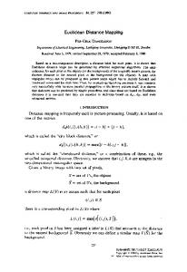
Fig. 1 shows how EDM is applied for phase analysis at interfaces using a BSE image of the paste

85

region adjacent to an aggregate particle (Fig. 1a) as an example. To determine the porosity gradient from the 3


aggregate boundary, first, the binary mask of the pore (Fig. 1b) and aggregate (Fig. 1c) phase is created. Next, an

87

EDM of the paste (Fig. 1d) is generated from the aggregate binary mask. Then, a multiplicative operation is

88

performed between the paste EDM and the pore mask, giving an EDM of the pore phase only (Fig. 1e). Observe

89

that each pore pixel in the original binary image is now transformed to a grey value that has a numerical value

90

equal to its linear distance to the nearest aggregate pixel, i.e. a particular pore pixel with grey value of x is

91

located x pixels away from the nearest aggregate boundary.

92

a) BSE image of a paste region adjacent to an aggregate particle. Field of view: 100 x 120μm

b) Pore binary mask.

d) EDM of paste from the aggregate boundary. The grey value of each pixel in the paste increases with its nearest distance from the boundary. 93

c) Aggregate binary mask

e) Distance map of the pore phase from the aggregate boundary. The brightness of each pore pixel represents its nearest distance to the aggregate.

Figure 1 Generating a Euclidean Distance Map (EDM) of the pore phase from the aggregate boundary. 4


Next, the brightness histogram of the paste and pore EDM are plotted in Figs. 2a and 2b respectively.

95

Normalising the brightness histogram of the pore EDM to the paste EDM, and converting the grey values to

96

actual distances by factoring with the pixel spacing, gives the porosity distribution from the interface at a single

97

pixel step (Fig. 2c). From this data, the porosity distribution can be re-plotted at any strip width, if desired. Fig.

98

2d gives an example where the porosity gradient is re-plotted at 5μm intervals.

99

250 200

525

Number of pixels

Number of pixels

550

500

475

150 100

50

450

0

0

50

100

150

200

250

0

Grey value

150

200

250

b) Brightness histogram of Fig. 1(e). The grey value 0 (black) representing the solid phase is not plotted.

45

45

40

40

Detectable porosity (%)


100

Grey value

a) Brightness histogram of Fig. 1(d). The grey value 255 (white) representing aggregate is not plotted.

35 30 25 20 15 10

35 30 25 20 15 10 5

5

0

0 0

10

20

30

40

50

60

Distance from aggregate (µm)

c) Porosity distribution from interface at 1pixel (0.26μm) strip width.

100

50

5 10 15 20 25 30 35 40 45 50 55 60 65 Distance from aggregate (µm)

d) Porosity distribution from interface at 5μm strip width resolution. The y-error bars represent relative standard error ( 1 / N ), where N is the number of pore pixels counted.

Figure 2 Use of EDM for quantitative phase analysis at the aggregate-paste interface

101 102

Another advantage of the new method is that it is easily applied on any geometry and boundary

103

conditions. A BSE image of an OPC concrete is shown in Fig. 3a. Note the random nature of the paste and the 5


range of separation distances between aggregates. As mentioned earlier, unless the strips are generated manually,

105

the conventional dilation-subtraction strip method can only be applied where the separation distance between

106

adjacent boundaries are at least twice the distance to the furthest strip, typically around 50μm. Therefore, for the

107

example in Fig. 3a, only the lower half of the image is suitable for strip analysis. This can create biased sampling

108

and non-representative results, no matter how many images are averaged. Figs. 3b-d show that the new method

109

is applicable to any paste geometry easily, thus all areas are included. Note that there is an uncertainty in the

110

distance map for features near the image border because influences from aggregate particles outside the image

111

have not been accounted for. Therefore, in Figs. 3b and 3c, the distance maps are cropped by an amount equal to

112

the distance of the furthest ‘strip’, in this case 50μm.

a) Concrete (w/c 0.5). The white border represents the 50μm strip. Field of view: 267 x 200μm

b) EDM of paste from aggregate boundary. The phase analysis is confined to features located 50μm from the edge of the image, i.e. contained in the box. 35


Detectable porosity

30

+/- Relative error

25 20 15 10 5 0 0

5

10 15 20 25 30 35 40 45 50 Distance from aggregate (µm)

c) Distance map of pores.

113 114 115

d) Porosity distribution from interface at 1 pixel (0.26μm) strip width.

Figure 3 Applying the EDM method on a random section of an OPC concrete. The porosity distribution from the aggregate-paste interface is obtained by normalising the brightness histogram of the pore EDM to the brightness histogram of the paste EDM. 6


3.

Example of application

117

In this section, the new method will be used to investigate spatial distribution of detectable porosity and

118

anhydrous cement at the ITZ. For this purpose, an OPC concrete at water-cement ratio 0.4 was prepared. A

119

cylindrical sample (100Φ x 250mm) was cast, demoulded after 24 hours and wrapped in cling film for 3 days.

120

After curing, an 8mm thick disc was cut from approximately 100mm from the bottom cast face, from which a

121

block sample (40 x 20mm) was sectioned. The block was freeze-dried, vacuum-impregnated with a low viscosity

122

epoxy, ground and polished using successively finer grit size down to ¼µm. To ensure a deep epoxy penetration,

123

the vacuum impregnated sample was pressurised at 2.5bar above atmosphere for 30 minutes [7]. A non-aqueous

124

solution was used as lubricant for cutting and polishing. Acetone was used as cleaning fluid.

125

A JEOL 5410LV scanning electron microscope, operated at low vacuum (9Pa), 10kV accelerating

126

voltage and 10mm free working distance was used for imaging. Thirty images (1024 x 768 pixels, pixel spacing

127

0.26μm) were captured at 500x magnification. In order to minimise risk of local variation, the sampling

128

procedure should obtain many images taken at different locations, dispersed over a large area and different

129

aggregate particles. Thus, a uniform random sampling procedure was adopted. The microscope stage was

130

programmed to move in a grid, stopping at thirty predefined, equally spaced coordinates spanning the entire

131

sample. If a frame fell entirely on an aggregate particle or entirely on paste, it was replaced by another location

132

within the neighbouring grids, chosen from a random number table.

133

Each image was captured with a constant brightness and contrast settings for reproducibility. The

134

brightness and contrast were calibrated with an aluminium-epoxy microanalytical standard so that the image

135

greyscale histogram was stretched to cover the entire greyscale, but not over-saturated at the low and high ends

136

of the spectrum. The pore phase was segmented using the ‘overflow’ method [8]; the inflection point of the

137

cumulative brightness histogram was taken as the upper threshold grey value for pores. The anhydrous cement

138

phase was segmented by using the minimum point between the peaks for hydrated paste and anhydrous phase as

139

the lower threshold value. Bond cracks appearing at the interface and air voids were excluded from the analysis.

140

We have decided not to analyse the calcium hydroxide (CH) phase due to problems in segmentation. The grey

141

values for CH and other hydrated phases tend to overlap significantly and it is very difficult to confidently

142

isolate these on the basis of grey value alone. As mentioned by Scrivener et al. [2], the distance measured on a

143

random plane section will overestimate the true normal distance from the aggregate surface. In this work, no

144

attempt was made to correct for this effect and all distances are reported as measured.

7


Fig. 4 shows the distribution of anhydrous cement particles and detectable porosity from the aggregate-

146

paste interface at one pixel strip width. Results are expressed as area percentage of the cement paste. Fig. 4a

147

clearly shows a deficit in cement grains near the boundary compared to bulk paste. The very pronounced

148

anhydrous cement gradient is due to disrupted packing of cement grains against much larger aggregate particles,

149

i.e. the ‘wall-effect’, which is generally regarded as the basis of the ITZ phenomena. The anhydrous cement

150

fraction increased steadily from 1% at the boundary to around 14% at 50μm away. However, the distribution of

151

detectable porosity from the interface, shown in Fig. 4(b), gave interesting results. At less than 5μm away from

152

the interface, there appears to be a sudden drop in detectable porosity, giving an impression that the aggregates

153

are surrounded by a thin layer of paste that is almost as dense as the bulk paste. We note that this feature has not

154

been reported before, possibly because previous studies were at lower resolution. Nevertheless, the general trend

155

is conventional; porosity decreases with increasing distance from the interface and the value at the boundary is

156

approximately twice that of the bulk region. From Fig. 4, it appears that the ITZ extends to around 50μm away

157

from the aggregate surface, with respect to both anhydrous cement and detectable porosity gradients.

158

After a thorough check on all the images and individual porosity gradients, we observed three types of

159

ITZ characteristics, shown in Fig. 5. The first appears to be a very porous ITZ, with a strong porosity gradient,

160

the detectable porosity at the interface almost three times that of the bulk paste. This may be similar to the ITZs

161

originally reported by Scrivener et al. [1, 2]. The second is much denser with large amounts of CH deposited on

162

the aggregate surface. The detectable porosity gradient is weak and there is a sudden drop in porosity at less than

163

5μm from the aggregate surface due to the presence of CH. This may be similar to that reported by Diamond and

164

Huang [9, 10]. The third type contains a mixture of ‘porous’ and ‘dense’ ITZs; the porosity gradient is evident,

165

but is not as strong as the first example. Obviously, the ‘average’ porosity gradient of the ITZ will depend on the

166

relative proportion of the ‘porous’ and ‘dense’ ITZs contained in the sample set. However, the presence, size and

167

shape of CH deposits are very irregular; we observed that some aggregate particles are almost completely lined

168

with CH in the 2D observation plane, while others are entirely free of it. Therefore, the sampling method will

169

also have an influence on the measured ‘average’ porosity gradient. For example, results obtained from studies

170

that adopt a uniform random sampling method, e.g. Scrivener et al [1, 2] will be different from those that select

171

an aggregate particle and then capture a succession of adjacent images around the chosen grain, e.g. Diamond

172

and Huang [9, 10]. This could be the reason why in the study by Diamond and Huang [10], high porosity was not

173

observed within the first 5μm of the aggregate surface.

174 8

18

28

16

26

14 12 10 8 6 4

Anhydrous cement

2


Anhydrous cement (%)

Cement & Concrete Research (2006), 36 (6) 1091-1097

Detectable porosity +/- Relative error

24 22 20 18 16 14

+/- Relative error

0

12 0

5

10 15 20 25 30 35 40 45 50

0

5



(a) 175 176

(b)

Figure 4 Detectable anhydrous cement (a) and porosity distribution (b) plots at single pixel strip width, measured from the aggregate-paste interface. Values are the average of 30 frames.

177

C

B


A

60 55 50 45 40 35 30 25 20 15 10 5 0

A B C

0

5


178 179 180 181 182

Figure 5 Detectable porosity distribution plots showing different ITZ characteristics: A) very porous ITZ; B) relatively dense ITZ with large amount of CH deposits on the aggregate surface (arrowed); and C) mixture of porous and dense ITZs. The averaged result will depend on the relative proportion of the porous and dense ITZ. Note that the bond cracks visible in A and C are not tallied. White border represents the 50μm strip (field of view: 267 x 200μm).

9


Another important issue is the degree of variability in the observed microstructural gradients at different

184

locations. Although the deficiency in anhydrous cement and excess in detectable porosity at the ITZ is evident

185

and clearly seen in the averaged results, there is however, a significant variability from location to location. Fig.

186

6 shows the coefficient of variation for the mean anhydrous cement and detectable porosity, plotted against

187

distance from the aggregate surface. The coefficient of variation ranges between 30 and 60% for detectable

188

porosity and between 60 and 120% for anhydrous cement. It is noted that the variability is particularly high in

189

the first 5μm from the aggregate surface and this is likely to be due to the variability in the amount of CH

190

deposited on aggregate particles. We also note that the size of the ‘CH influence zone’ as observed in Fig. 6

191

matches that of the one in the porosity gradient (Fig. 4b). However, it is stressed that the number of samples

192

investigated in this study is limited and the results are preliminary. Nevertheless, the high variability in the

193

microstructural gradients is real and as emphasised by Diamond and Huang [9, 10], must be given consideration

194

in computer models that attempt to simulate the microstructure of cement-based materials.

Coefficient of variation (%)

120 100 80 60 40 Detectable porosity

20

Anhydrous cement

0 0

5

10 15 20 25 30 35 40 45 50


195 196 197 198

Figure 6 Coefficients of variation for the average detectable porosity and anhydrous cement plotted against distance from aggregate surface. Note the high variability, particularly at less than 5μm from the aggregate surface.

199 200

4.

Conclusion

201

A new image analysis method for investigating microstructural gradients at interfaces in composite materials is

202

presented. The method uses Euclidean Distance Mapping to generate microstructural gradient plots at single-

203

pixel strip width. The new method is faster and more flexible than conventional dilation-subtraction strip

204

analysis, and is not constrained by feature geometry and boundary conditions. Therefore a truly random and

205

unbiased sampling procedure can be achieved. The new method was applied to investigate microstructural 10


gradients at the interfacial transition zone of an ordinary Portland cement concrete sample. The results showed

207

that although the overall ITZ can be characterised by a strong gradient in anhydrous cement and detectable

208

porosity, this is highly variable from location to location. The higher sensitivity of the new method enabled it to

209

detect previously unreported effects of calcium hydroxide deposits on the aggregate surface on the porosity

210

gradient. The measured ‘average’ characteristic of the ITZ via image analysis is dependent upon the extent of

211

CH deposition at aggregate surfaces and also on the adopted sampling procedure.

212 213

Acknowledgements

214

HSW would like to acknowledge the financial assistance provided by the Universities UK, via the Overseas

215

Research Students Awards Scheme. We thank Mr. R.A. Baxter for his help with the laboratory work.

216 217

References

218

[1]

219 220

particles, Mat Res Soc Symp Proc, 114, 77-86. [2]

221 222

K.L. Scrivener, A.K. Crumbie, P.L. Pratt, (1988) A study of the interfacial region between cement paste and aggregate in concrete, Mat Res Soc Symp Proc, 114, 87-88.

[3]

223 224

K.L. Scrivener, E.M. Gartner (1988), Microstructural gradients in cement paste around aggregate

K.L. Scrivener, A. Bentur, P.L. Pratt (1988), Quantitative characterisation of the transition zone in high strength concrete, Advances in Cement Research, 1 [4] 230-237.

[4]

225

P.E. Danielsson (1980), Euclidean distance mapping, Computer, Graphics and Image Processing, 14, 227-248.

226

[5]

A. Rosenfeld, J. Pfaltz (1968), Distance functions on digital pictures, Pattern Recognition, 1, 33-61.

227

[6]

J.C. Russ (2002), The Image Processing Handbook, Fourth edition, CRC Press, London, 744p.

228

[7]

H.S. Wong, N.R. Buenfeld, Patch microstructure in cement-based materials: Fact or artefact? Cem.

229 230 231

Concr. Res. (accepted for publication), 2005. [8]

H.S. Wong, M.K. Head, N.R. Buenfeld, Pore segmentation of cement-based materials from backscattered electron images, Cem. Concr. Res. (accepted for publication), 2005.

11


[9]

S. Diamond, J. Huang (1998), Interfacial transition zone: reality or myth? In: A. Katz, A. Bentur. M.

233

Alexander, G. Arliguie (Eds.), Proc. RILEM 2nd Int. Conf. On the Interfacial Transition Zone in

234

Cementitious Composites, RILEM Publications SARL, Paris, 35, 1-40.

235 236

[10]

S. Diamond, J. Huang (2001), The ITZ of concrete – a different view based on image analysis and SEM observations, Cem. Concr. Compos., 23, 179-188.

12

Euclidean Distance Mapping for computing microstructural gradients ...

Euclidean Distance Mapping for computing microstructural gradients ...

Suggest Documents