Evaluating Algorithm Performance Metrics Tailored for ... - CiteSeerX

Evaluating Algorithm Performance Metrics Tailored for Prognostics Abhinav Saxena Research Institute for Advanced Computer Science 650-604-3208 [email protected]

José Celaya Research Institute for Advanced Computer Science 650-604-4596 [email protected]

Sankalita Saha Research Institute for Advanced Computer Science 650-604-4593 [email protected]

Bhaskar Saha Mission Critical Technologies, Inc. 650-604-4379 [email protected]

Kai Goebel National Aeronautics and Space Administration 650-604-4204 [email protected]

Prognostics Center of Excellence NASA Ames Research Center, Moffett Field CA 94035 8. CONCLUSION.................................................................... 9 REFERENCES...................................................................... 10 BIOGRAPHIES..................................................................... 10

Abstract—Prognostics has taken center stage in Condition Based Maintenance (CBM) where it is desired to estimate Remaining Useful Life (RUL) of the system so that remedial measures may be taken in advance to avoid catastrophic events or unwanted downtimes. Validation of such predictions is an important but difficult proposition and a lack of appropriate evaluation methods renders prognostics meaningless. Evaluation methods currently used in the research community are not standardized and in many cases do not sufficiently assess key performance aspects expected out of a prognostics algorithm. In this paper we introduce several new evaluation metrics tailored for prognostics and show that they can effectively evaluate various algorithms as compared to other conventional metrics. The four prognostic algorithms are Relevance Vector Machine (RVM), Gaussian Process Regression (GPR), Artificial Neural Network (ANN), and Polynomial Regression (PR) are compared. These algorithms vary in complexity and their ability to manage uncertainty around predicted estimates. Results show that the new metrics rank these algorithms in a different manner; depending on the requirements and constraints suitable metrics may be chosen. Beyond these results, this paper offers ideas about how metrics suitable to prognostics may be designed so that the evaluation procedure can be standardized. 1 2

1. INTRODUCTION Prognostics is an emerging concept in condition based maintenance (CBM) of critical systems. Along with developing the fundamentals of being able to confidently predict Remaining Useful Life (RUL), the technology calls for fielded applications as it inches towards maturation. This requires a stringent performance evaluation so that the significance of the concept can be fully understood. Currently, prognostics concepts lack standard definitions and suffer from ambiguous and inconsistent interpretations. This lack of standards is in part due to the varied end-user requirements for different applications, a wide range of time scales involved, available domain information, domain dynamics, etc. to name a few issues. The research community has used a variety of metrics based largely on convenience with respect to their respective requirements. Very little attention has been focused on establishing a common ground to compare different efforts. This paper builds upon previous work that surveyed metrics in use for prognostics in a variety of domains including medicine, nuclear, automotive, aerospace, and electronics. [1]. The previous effort suggested a list of metrics to assess critical aspects of RUL predictions. This paper will show how such metrics can be used to assess the performance of prognostic algorithms. Furthermore, it will assess whether these metrics capture the performance criteria for which they were designed. The paper will focus on metrics that are specifically designed for prognostics beyond conventional metrics currently being used for diagnostics and other forecasting applications. These metrics in general address the issue of how well the RUL prediction estimates improve

TABLE OF CONTENTS 1. INTRODUCTION.................................................................1 2. MOTIVATION ....................................................................2 3. PREVIOUS WORK .............................................................2 4. APPLICATION DOMAIN ....................................................3 5. ALGORITHMS EVALUATED ..............................................3 6. PERFORMANCE METRICS ................................................5 7. RESULTS & DISCUSSION ..................................................7 1 1 U.S. Government work not protected by U.S. copyright. 2

IEEEAC paper #1387, Version 1, Updated November 2, 2008

1

compare different algorithms. With these ideas we hope to provide some starting points for future discussions.

over time as more measurement data become available. A good prognostic algorithm should not only improve in RUL estimation but also ensure a reasonable prediction horizon and confidence levels on the predictions.

3. PREVIOUS WORK

Overall the paper is expected to enhance a general understanding of these metrics so that they can be further refined and be accepted by the research community as standard metrics for the performance assessment of prognostics algorithms.

In a recent effort a thorough survey of various application domains that employ prediction related tasks was conducted [1]. The central idea there was to identify established methods of performance evaluation in the domains that can be considered mature and already have fielded applications. Specifically, domains like medicine, weather, nuclear, finance and economics, automotive, aerospace, electronics, etc. were considered. The survey revealed that although each domain employs a variety of custom metrics, metrics based on accuracy and precision dominated the landscape. However, these metrics were often used in different contexts depending on the type of data available and the kind of information derived from them. This suggests that one must interpret the usage very carefully before borrowing any concepts from other domains. A brief summary of the findings is presented here for reference.

2. MOTIVATION Prognostics technology is reaching a point where it must be evaluated in real world environments in a truly integrated fashion. This, however, requires rigorous testing and evaluation on a variety of performance measures before they can be certified for critical systems. For end-of-life predictions of critical systems, it becomes imperative to establish a fair amount of faith in the prognostic systems before incorporating their predictions into the decisionmaking process. Furthermore, performance metrics help establish design requirements that must be met. In the absence of standardized metrics it has been difficult to quantify acceptable performance limits and specify crisp and unambiguous requirements to the designers. Performance evaluation allows comparing different algorithms and also yields constructive feedback to further improve these algorithms.

Domains like medicine and finance heavily utilize statistical measures. These domains benefit from availability of large datasets under different conditions. Predictions in medicine are based on hypothesis testing methodologies and metrics like accuracy, precision, interseparability, and resemblance are computed on test outcomes. In finance, statistical measures are computed on errors calculated based on reference prediction models. Metrics like MSE (mean squared error), MAD (mean absolute deviation), MdAD (median absolute deviation), MAPE (mean absolute percentage error), and their several variations are widely used. These metrics represent different ways of expressing accuracy and precision measures. The domain of weather predictions mainly uses two classes of evaluation methods, error-based statistics and measures of resolution between two outcomes. A related domain of wind mill power prediction uses statistical measures already listed above. Other domains like aerospace, electronics, and nuclear are relatively immature as far as fielded prognostics applications are concerned. In addition to conventional accuracy and precision measures, a significant focus has been on metrics that assess business merits like ROI (return on investment), TV (technical value), life cycle cost other than reliability based metrics like MTBF (mean time between failure) or the ratio MTBF/MTBUR (mean time between unit replacements).

Performance evaluation is usually the foremost step once a new technique is developed. In many cases benchmark datasets or models are used to evaluate such techniques on common ground so they can be fairly compared. Prognostic systems, in most cases, have neither of these options. Different researchers have used different metrics to evaluate their algorithms, making it rather difficult to compare various algorithms even if they have been declared successful based on their respective evaluations. It is accepted that prognostics methods must be tailored for specific applications, which makes it difficult to develop a generic algorithm useful for every situation. In such cases customized metrics may be used but there are characteristics of prognostics applications that remain unchanged and corresponding performance evaluation can establish a basis for comparisons. So far very little has been done to identify common ground when it comes to testing and comparing different algorithms. In two surveys of methods for prognostics (one of data-driven methods and one of artificial-intelligence-based methods) [2, 3], it can be seen that there is a lack of standardized methodology for performance evaluation and in many cases performance evaluation is not even formally addressed. Even the ISO standard [4] for prognostics in condition monitoring and diagnostics of machines lacks a firm definition of such metrics. Therefore, in this paper we present several new metrics and show how they can be effectively used to

Several classifications of these metrics have been presented in [1] that are derived from the end use of the prognostics information. It has been argued that depending on the end user requirements one must choose appropriate sets of these metrics or their variants to appropriately evaluate the performance of the algorithms.

2

4. APPLICATION DOMAIN

of EIS measurements to compute RE+RCT and then uses prediction algorithms to predict evolution of these parameters. RE+RCT have been shown to be directly related to battery capacity and hence their evolution curve can be easily transformed into battery RUL. Another approach directly tracks battery capacity and trends it to come up with RUL estimates. In the next sections we describe our prediction algorithms and the corresponding approaches that were used to estimate battery life.

In this section we describe the application domain we used to show how these new prognostics metrics can be used to compare different algorithms. INL Battery Dataset In 1998 the Office of Vehicle Technologies at the U.S. Department of Energy initiated the Advanced Technology Development (ATD) program in order to find solutions to the barriers limiting commercialization of high-power Lithium-ion batteries for hybrid-electric and plug-in electric vehicles. Under this program, a set of second-generation 18650-size Lithium-ion cells were cycle-life tested at the Idaho National Laboratory (INL).

Battery Capacity Decay with Time

Capacity (AmpHr)

0.95

The cells were aged under different experimental settings like temperature, State-of-Charge (SOC), current load, etc. Regular characterization tests were performed to measure behavioral changes from the baseline under different aging conditions. The test matrix consisted of three SOCs (60, 80, and 100%), four temperatures (25, 35, 45, and 55˚C), and three different life tests (calendar-life, cycle-life, and accelerated-life) [5]. Electrode Impedance Spectroscopy (EIS) measurements were recorded every four weeks to estimate battery health. EIS measurements were then used to extract internal resistance parameters (electrolyte resistance: RE and charge transfer resistance: RCT, see Figure 1) that have been shown to empirically characterize ageing characteristics using a lumped parameter model for the Liion batteries [6].

RE+RCT (Ω )

0.8 0.75

Failure Threshold

0.7

0

8

16

24

32 40 Time (weeks)

48

56

64

72

Figure 2 – Battery capacity decay profile at 45°C.

5. ALGORITHMS EVALUATED In this effort we chose four data-driven algorithms to show the effectiveness of various metrics in evaluating their performance. These algorithms range from simple polynomial regression to sophisticated Bayesian learning methods. The approaches used here have been described before in [6, 7], but they are repeated here for the sake of completeness and readability. Also mentioned briefly is the procedure for how each of these algorithms was applied to the battery health management dataset.

0.035

Polynomial Regression (PR) Approach

0.03

We employed a simple data-driven routine to establish a baseline for battery health prediction performance and uncertainty assessment. For this data-driven approach, as the first step, the equivalent damage threshold in the RE+RCT (dth=0.033) is gleaned from the relationship between RE+RCT and the capacity C at baseline temperature (25ºC). Next, via extracted features from the EIS measurements, RE+RCT was tracked at elevated temperatures (here 45ºC). Ignoring the first two data points (which behave similar to what is considered as “wear-in” pattern in other domains), a second degree polynomial was used at the prediction points to extrapolate out to the damage threshold. This linear extrapolation is then used to compute the expected RUL values.

0.025 0.02 0.015

0.85

0.65

Battery Internal Resistance Parameters (RE + RCT)

0.04

EOL (64.46 weeks)

0.9

0

8

16

24

32 40 Time (weeks)

48

56

64

72

Figure 1 – Internal parameter values are used as features extracted from EIS measurements to characterize battery health. As shown in Figure 2, battery capacity was also measured in ampere hours by measuring time and currents during discharge cycle for the batteries. For the data used in our study, the cells were aged at 60% SOC and at temperatures of 25°C and 45°C. The 25°C data is used solely for training while the 45°C data is used for both training as well as testing.

Relevance Vector Machines (RVM) The Relevance Vector Machine (RVM) [8] is a Bayesian form representing a generalized linear model of the Support Vector Machine (SVM) with identical functional form [9]. Although, SVM is a state-of-the-art technique for

Different approaches can be taken to predict battery life based on the above measurements. One approach makes use 3

m( x ) = Ε[ f ( x )], k ( x, x ' ) = Ε[( f ( x) − m( x ))( f ( x') − m( x ' ))], and

classification and regression, it suffers from a number of disadvantages, one of which is the lack of probabilistic outputs that make more sense in health monitoring applications. The RVM attempts to address these very issues in a Bayesian framework. Besides the probabilistic interpretation of its output, it typically uses a lot fewer kernel functions for comparable generalization performance.

f ( x) ~ GP (m( x), k ( x, x')). The index set X ∈ ℜ is the set of possible inputs, which need not necessarily be a time vector. Given prior information about the GP and a set of training points {(xi,fi)| i = 1,…,n}, the posterior distribution over functions is derived by imposing a restriction on prior joint distribution to contain only those functions that agree with the observed data points. These functions can be assumed to be noisy as in real world situations we have access to only noisy observations rather than exact function values, i.e. yi = f(x) + , where is additive IID N(0, n2). Once we have a posterior distribution it can be used to assess predictive values for the test data points. Following equations describe the predictive distribution for GPR [11].

This type of supervised machine learning starts with a set of input vectors {xn}, n = 1,…, N, and their corresponding targets {tn}. The aim is to learn a model of the dependency of the targets on the inputs in order to make accurate predictions of t for unseen values of x. Typically, the predictions are based on some function F(x) defined over the input space, and learning is the process of inferring the parameters of this function. The targets are assumed to be samples from the model with additive noise:

t n = F (x n ; w ) + ε n

(1)

Prior y

where, n are independent samples from some noise process (Gaussian with mean 0 and variance 2). Assuming the independence of tn, the likelihood of the complete data set can be written as: p (t | w , σ ) = ( 2πσ ) 2

2 −N / 2

exp −

1 2σ

2

t − Φw

2

f test

~ N 0,

K ( X , X ) + σ n2 K ( X , X test ) K ( X test , X ) K ( X test , X test )

(5)

Posterior f test | X , y , X test ~ N ( f test , cov( f test )), where

(2)

f test ≡ Ε[ f test | X , y , X test ] = K ( X , X test )[ K ( X , X ) + σ n2 I ] −1 y ,

(6)

cov( f test ) = K ( X test , X test ) − [ K ( X test , X ) + σ n2 I ] −1 K ( X , X test ).

where, w = (w1, w2,…, wM)T is a weight vector and is the N x (N+1) design matrix with = [ (t1), (t2), … (tN),]T; in which (tN) = [1, K(xn,x1), K(xn,x2), …, K(xn,xN)]T, K(x,xi) being a kernel function.

A crucial ingredient in a Gaussian process predictor is the covariance function (K(X, X’)) that encodes the assumptions about the functions to be learnt by defining the relationship between data points. GPR requires a prior knowledge about the form of covariance function, which must be derived from the context if possible. Furthermore, covariance functions consist of various hyper-parameters that define their properties. Setting right values of such hyper-parameters is yet another challenge in learning the desired functions. Although the choice of covariance function must be specified by the user, corresponding hyper-parameters can be learned from the training data using a gradient based optimizer such as maximizing the marginal likelihood of the observed data with respect to hyper-parameters [12].

To prevent over-fitting a preference for smoother functions is encoded by choosing a zero-mean Gaussian prior distribution over w parameterized by the hyperparameter vector . To complete the specification of this hierarchical prior, the hyperpriors over and the noise variance 2 are approximated as delta functions at their most probable values MP and 2MP. Predictions for new data are then made according to: 2 2 p(t* | t ) = p(t* | w, σ MP ) p (w | t,η MP , σ MP )dw.

(4)

(3)

We used GPR to regress the evolution of internal parameters (RE+RCT) of the battery with time. Relationship between these parameters and the battery capacity was learned from experimental data [7]. Thus the internal parameters were regressed for the data obtained at and the corresponding estimates were translated into estimated battery capacity at 45ºC using the relationship learnt at 25ºC.

Gaussian Process Regression (GPR) Gaussian Process Regression (GPR) is a probabilistic technique for nonlinear regression that computes posterior degradation estimates by constraining the prior distribution to fit the available training data [10]. A Gaussian Process (GP) is a collection of random variables any finite number of which have a joint Gaussian distribution. A real GP f(x) is completely specified by its mean function m(x) and covariance function k(x,x’) defined as:

Neural Network (NN) Approach A neural network based approach was considered as an alternative data-driven approach for prognostics. A basic feed forward neural network with back propagation training was used; details on this algorithm can be found in [13, 14]. 4

As described earlier for the other approaches, data at 25oC was used to learn the relationship between internal parameter RE+RCT and the capacity C using the neural network NN1. In addition, the 45oC data was used as a test case. Here, measurements of the internal parameter RE+RCT are only available up to time tP (time at which RUL prediction is made). The available RE+RCT measurements are extrapolated after time tP in order to predict future values. This extrapolation is done using neural network NN2 which learns the relationship between RE+RCT and time. Once future values for RE+RCT are computed using NN2 these RE+RCT values are the used as an input to NN1 in order to obtain C.

(MAPE). These metrics have been included to illustrate how these metrics are useful but may not capture time varying aspects of prognostic estimates. Further, five new metrics have been introduced that inclu such features of interest. These metrics have been first defined briefly and then evaluated based on the results for battery health management as presented in the following section. Terms and Notations • UUT is the unit under test •

∆l (i ) is the error between the predicted and the true RUL

at time index i for UUT l.

The structure of NN1 consists of two hidden layers with one and three nodes respectively. For the hidden layers tansigmoid transfer functions and for the output layers logsigmoid transfer functions were chosen. Training considers random initial weights, a reduced memory LevenbergMarquardt algorithm, 200 training epochs, and meansquared error as a performance parameter.

• EOP (End-of-Prediction) is the earliest time index, i, after prediction crosses the failure threshold. • EOL represents End-of-Life, the time index for actual end of life defined by the failure threshold. • P is the time index at which the first prediction is made by the prognostic system.

The structure and training parameters of the NN2 remained fixed during the forecasting. The net was trained with data available up to week 32, and then the resulting model was used to extrapolate RE+RCT until tEOP is reached or it is clear that it will not be reached if the model does not converge. Once the next measurement point is available at week 36, the net was trained again including the new data point. The resulting model was used to extrapolate RE+RCT from tp+1=36 onwards. It is not expected that a fixed net structure and fixed training settings could perform optimally for all the training instances as measurements become available week 32 onwards. To make sure the results are acceptable for all the training instances, the initial weights were set to random and the training was repeated 30 times. This allowed the exploration of with different initial values in the optimization of the weights and allowed the exploration of different local minimums. The results of the 30 training cases were aggregated on the extrapolated values by computing the median. Cases were observed where the training stopped prematurely resulting in a net with poor performance, these cases were regarded as outliers and the use of the median was intended to diminish the impact of such outliers while aggregating all the training cases. The structure of NN2 consists of one hidden layer with three nodes, and tan-sigmoid transfer functions for all the layers. Training considers random initial weights, a reduced memory Levenberg-Marquardt algorithm, 200 training epochs, and mean-squared error as a performance parameter.

• rl(i) is the RUL estimate for the lth UUT at time ti as determined from measurement and analysis. •

r*l (i ) is the true RUL at time ti given that data is

available up to time ti for the lth UUT. •

is the cardinality of the set of all time indices at which the predictions are made, i.e. = (i | P ≤ i ≤ EOP ) .

Average Bias (Accuracy) Average bias is one of the conventional metrics that has been used in many ways as a measure of accuracy. It averages the errors in predictions made at all subsequent times after prediction starts for the lth UUT. This metric can be extended to average biases over all UUTs to establish overall bias. Bl =

1

∆l ( i ) .

(7)

i =1

Sample Standard Deviation (Precision) Sample standard deviation measures the dispersion/spread of the error with respect to the sample mean of the error. This metric is restricted to the assumption of normal distribution of the error. It is, therefore, recommended to carry out a visual inspection of the error plots to determine the distribution characteristics before interpreting this metric.

6. PERFORMANCE METRICS In this section nine different performance metrics are described. Four of them are the metrics most widely used in the community, i.e., accuracy, precision, Mean Squared Error (MSE), and Mean Absolute Percentage Error

S=

5

i =1

(∆(i) − m)2 −1

(8)

within specified limits around the actual EOL and hence the predictions may be considered trustworthy. It is expected that PHs are determined for an algorithm-application pair offline during the validation phase and then these numbers be used as guidelines when the algorithm is deployed in test application where actual EOL are not known in advance. While comparing algorithms, an algorithm with longer prediction horizon would be preferred.

where m is the sample mean of the error. Mean Squared Error (MSE) Simple average bias metric suffers from the fact that negative and positive errors cancel each other and high variance may not be reflected in the metric. Therefore, MSE averages the squared prediction error for all predictions and encapsulates both accuracy and precision. A derivative of MSE, often used, is Root Mean Squared Error (RMSE).

1

∆ (i ) 2 .

{

i =1

For prediction applications it is important to differentiate between errors observed far away from the EOL and those that are observed close to EOL. Smaller errors are desirable as EOL approaches. Therefore, MAPE weighs errors with RULs and averages the absolute percentage errors in the multiple predictions. Instead of the mean, median can be used to compute Median absolute percentage error (MdAPE) in a similar fashion. 1 i =1

100∆(i ) . r* (i )

)}

For instance, a PH with error bound of = 5% identifies when a given algorithm starts predicting estimates that are within 5% of the actual EOL. Other specifications may be used to derive PH as desired.

Mean Absolute Percentage Error (MAPE)

MAPE =

(

where i = min j | ( j ∈ ) ∧ r* (1 − α ) ≤ r l ( j) ≤ r* (1 + α ) .

(9)

- Accuracy Another way to quantify prediction quality may be through a metric that determines whether the prediction falls within specified accuracy levels at particular times. These time instances may be specified as percentage of total remaining life from the point the first prediction is made or a given absolute time interval before EOL is reached. In our implementation we define - accuracy as the prediction accuracy to be within *100% of the actual RUL at specific time instance t expressed as a fraction of time between the point when an algorithm starts predicting and the actual failure. For example, this metric determines whether a prediction falls within 20% accuracy (i.e., =0.2) halfway to failure from the time the first prediction is made (i.e., =0.5).

(10)

It must be noted that the above metrics can be more suitably used in cases where either a distribution of RUL predictions is available as the algorithm output or there are multiple predictions available from several UUTs to compute the statistics. Whereas these metrics can convey meaningful information in these cases, these metrics are not designed for applications where RULs are continuously updated as more data is available. It is desirable to have metrics that can characterize improvement in the performance of a prognostic algorithm as time approaches near end-of-life. In this paper we discuss one such application where algorithms are tracking battery health and show how newer metrics can encapsulate such information which is valuable for successfully fielded application of prognostics. Therefore, next we discuss new metrics tailored for prognostics and show how they are more informative than the ones traditionally used.

[1 − α ] ⋅ r* (t ) ≤ r l (t λ ) ≤ [1 + α ] ⋅ r* (t ) where

(12)

α : accuracy modifier : time window modifier t λ = P + λ (EOL − P ) .

r*l (i )

Prediction Horizon has been in the literature for quite some time but no formal definition is available. The notion suggests that longer the prognostics horizon more time is available to act based on a prediction that has some credibility. We define Prognostic Horizon as the difference between the current time index i and EOP utilizing data accumulated up to the time index i, provided the prediction meets desired specifications. This specification may be specified in terms of allowable error bound ( ) around true EOL. This metric ensures that the predicted estimates are

r (i) α = 20%

RUL

Prognostic Horizon (PH)

- Accuracy l

λ=0

tP

Precision Spread

MSE =

(11)

H = EOP − i

r l (i )

λ = 0.5 Time Index (i)

λ =1

t EOL

Figure 3 – Schematic depicting - Accuracy.

6

Relative Accuracy (RA)

Let (xc, yc) be the center of mass of the area under the curve M(i). Then, the convergence CM can be represented by the Euclidean distance between the center of mass and (tp, 0), where

Relative prediction accuracy is a notion similar to accuracy where, instead of finding out whether the predictions fall within a given accuracy levels at a given time instant, we measure the accuracy level. The time instant is again described as a fraction of actual remaining useful life from the point when the first prediction is made. An algorithm with higher relative accuracy is desirable.

r* (tλ ) − r (tλ )

2

C M = ( xc − t P ) 2 + yc , xc =

1 EOP 2 2 (t i +1 − t i ) M (i ) 2 i=P EOP

l

RAλ = 1 −

(13)

r* (tλ )

i=P

yc =

where t λ = P + λ (EOL − P ) .

1 EOP (t i +1 − t i ) M (i ) 2 2 i=P EOP i=P

r l (i )

r*l (i )

RUL (i)

r l (i )

t EOL

Figure 4 – Schematic showing Relative Accuracy concept.

w( r l ) RAλ ,

yc ,1

1

Case 3

3

2

t EOP

Time Index (i)

Figure 5 – Schematic for the convergence of a metric.

Relative accuracy can be evaluated at multiple time instances. To aggregate these accuracy levels, we define Cumulative Relative Accuracy as a normalized weighted sum of relative prediction accuracies at specific time instances.

i =1

(t i +1 − t i ) M (i )

Case 2

t P xc,1

Cumulative Relative Accuracy (CRA)

1

.

Case 1 Metric M(i)

tλ

CRAλ =

(15)

M(i) is a non-negative prediction error accuracy or precision metric.

tλ

tP

, and

(t i +1 − t i ) M (i )

7. RESULTS & DISCUSSION As mentioned earlier, battery health measurements were taken every four weeks. Therefore, each algorithm was tasked to predict every four weeks after week 32, which gives eight data points to learn the degradation trend. Algorithms predict RULs until the end-of-prediction is reached, i.e. the estimates show that battery capacity has already hit 70% of the full capacity of one ampere hour. Corresponding predictions are then evaluated using all nine metrics. Estimates were available for all weeks starting week 32 through week 64. Algorithms like RVM always predicted conservatively, i.e. predicted a faster degradation than actually observed. Other algorithms like NN and PR started predicting at week 32 but could not predict beyond week 60 as their estimates had already crossed the failure threshold before that. GPR, however, required more training data before it could provide any estimates. Therefore, predictions for GPR start at week 48 and go until week 60.

(14)

where w is a weight factor as a function of RUL at all time indices. In most cases it is desirable to weigh the relative accuracies higher closer to the EOL. Convergence Convergence is defined to quantify the manner in which any metric like accuracy or precision improves with time to reach its perfect score. As illustrated below, three cases converge at different rates. It can be shown that the distance between the origin and the centroid of the area under the curve for a metric quantifies convergence. Lower distance means faster. Convergence is a useful metric since we expect a prognostics algorithm to converge to the true value as more information accumulates over time. Further, a faster convergence is desired to achieve a high confidence in keeping the prediction horizon as large as possible.

Table 1 – Performance evaluation for all four test algorithms with Error Bound = 5%. Bias SSD MSE MAPE

7

RVM -7.12 6.57 84.81 41.36

GPR 5.96 15.24 184.16 53.93

NN 5.04 6.81 59.49 37.54

PR 1.87 4.26 17.35 23.05

PH RA ( = 0.5) CRA ( = 0.5) Convergence

8.46 0.60 0.63 14.80

12.46 0.86 0.52 8.85

24.46 0.82 0.65 11.41

12.46 0.34 0.55 13.36

Table 2 – Performance evaluation for all four test algorithms for predictions made within prediction horizon with Error Bound = 5%.

Prediction Horizon (5% error) 50

actual RUL

GPR NN

PA 40

RUL

Bias SSD MSE MAPE PH RA ( = 0.5) CRA ( = 0.5) Convergence

95% accuracy zone End of Life (EOL) RVM RUL GPR RUL NN RUL

30

PA RUL

RVM

20

35

40

45

50

55

60

65

GPR -1.78 1.33 3.96 30.40 12.46 0.62 0.31 4.44

NN -1.53 1.45 3.27 27.44 12.46 0.69 0.33 4.61

PR 0.22 3.33 7.75 23.25 24.46 0.95 0.58 7.36

Another aspect of performance evaluation is the requirement specifications. As specifications change the performance evaluation criteria also changes. To illustrate this point, prediction horizon was now defined on a relaxed error bound of 10%. As expected, prediction horizons become longer for most of the algorithms and hence more predictions are taken into account while computing the metrics. Table 3 shows the results with the new prediction horizons and now the NN based approach also seems to perform well on several criteria. This means that for some applications where more relaxed requirements are acceptable simpler approaches may be chosen if needed.

10

0

RVM -1.19 1.18 2.03 39.33 8.46 0.77 0.50 3.76

70

Time (weeks)

Figure 6 – Predictions from different algorithms fall within the error bound at different times. In Table 1 results are aggregated based on all available predictions. These results clearly show that the polynomial fit approach outperforms all other algorithms in almost all cases. Even though the convergence properties are not the best they are comparable to the top numbers. However, using all predictions to compute these metrics results in a wide range of values, which makes it difficult to assess how other algorithms fare even if they may not necessarily be the best. Most metrics describe how close or far the predictions are to the true value but prediction horizon indicates when these predictions enter within the specified error bound and therefore may be trust worthy (see Figure 6). PR enters the error bound early on where as all other algorithms converge slowly as times passes by. The convergence metric encapsulates this attribute and shows that algorithms like GPR converge faster to better estimates and may be useful later on. We also learned that the current convergence metric does not take into account cases where algorithms start predicting at different time instances. In such cases algorithms that start predicting early on may have a disadvantage. Although this metric works well in most cases, a few adjustments may be needed to make it robust towards extreme cases.

Table 3 – Performance evaluation for all four test algorithms for predictions made within prediction horizon with Error Bound = 10%. Bias SSD MSE MAPE PH RA ( = 0.5) CRA ( = 0.5) Convergence

RVM -1.83 1.73 5.02 37.01 12.46 0.76 0.57 5.49

GPR 0.05 4.34 10.6 31.20 16.46 0.79 0.43 3.43

NN -1.53 1.45 3.27 27.44 12.46 0.69 0.33 4.61

PR 0.22 3.33 7.75 23.25 24.46 0.95 0.58 7.36

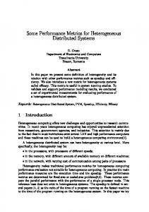
Figure 7 shows the - Accuracy metric for all four algorithms. Since all algorithms except GPR start prediction from week 32 onward, t is determined to be around 48.3 weeks. At that point only PR lies within 80% accuracy levels. GPR starts predicting week 44 onward, i.e. its t is determined to be around 54.3 week where it seems to meet the requirements. This metric signifies whether a particular algorithm reaches within a desired accuracy level halfway to the EOL from the point it starts predicting. Another aspect that may be of interest is whether an algorithm reaches the desired accuracy level some fixed time interval ahead of the EOL. In that case, for example, if t is chosen as 48 weeks then GPR will not meet the requirement. Therefore, this metric may be modified to incorporate cases where not all algorithms may be able to start predicting at the same time.

It must be pointed out that these metrics summarize all predictions, good or bad, into one aggregate, which may not be fair for algorithms that learn over time and get better later on. Therefore, next, it was decided to evaluate only those predictions that were made within the prediction horizon so that only the meaningful predictions are evaluated (Table 2). As expected the results change significantly and all the performance numbers become comparable for all algorithms. This provides a better understanding on how these algorithms compare. 8

α -λ Accuracy ( α = 0.2, λ = 0.5)

60

over late predictions. Finally, in the example discussed in this paper RUL estimates were obtained as a single value as opposed to a RUL distribution for every prediction. The metrics presented in this paper can be applied to applications where RUL distributions are available with slight modifications. Similarly for cases where multiple UUTs are available to provide data, minor adjustments will suffice.

End of Life (EOL) 80% accuracy zone

wk. 48.3

50

actual RUL RVM RUL GPR RUL NN RUL

RUL

40

PA RUL

30

wk. 54.3

20

8. CONCLUSION

10

In this paper we have shown how performance metrics for prognostics can be designed. Four different prediction algorithms were used to show how various metrics convey different kinds of information. No single metric should be expected to cover all performance criteria. Depending on the requirements a subset of these metrics should be chosen and a decision matrix should be used to rank different algorithms. In this paper we used nine metrics including four conventional ones that are most commonly used to evaluate algorithm performance. The new metrics provide additional information that may be useful in comparing prognostic algorithms. Specifically, these metrics track the evolution of prediction performance over time and help determine when these predictions can be considered trustworthy. Notions like convergence and prediction horizon that have existed in the literature for a long time have been quantified so they can be used in an automated fashion. Further, new notions of performance measures at specific time instances have been instantiated using metrics like relative accuracy and performance. These metrics represent the notion that a prediction is useful only if it is available so far in advance that it allows some time to mitigate the predicted contingency.

0

35

40

45

50

55

60

65

Time (weeks)

Figure 7 – The - Accuracy metric determines whether predictions are within the cone of desired accuracy levels at a given time instant (t ). Battery Capacity Decay with Time

Capacity (AmpHr)

0.95 0.9

(a)

0.85

(b)

0.8 0.75

Failure Threshold

0.7 0.65 0

8

16

24

32 40 Time (weeks)

48

56

64

72

Figure 8 – Battery capacity decay profile shows several features that are difficult to learn using simple regression techniques.

Whereas these metrics demonstrate several ideas specific to prognostics performance evaluation, we by no means claim this list of metrics to be near perfect. It is anticipated that as new ideas are generated and the metrics themselves are evaluated in different applications, this list will be revised and refined before a standard methodology can be devised for evaluating prognostics. This paper is intended to serve as a start towards developing such metrics that can better summarize prognostic algorithm performance.

It can be observed from the results (Figure 7) that most algorithms fail to follow the trend towards the end. These data-driven regression based techniques find it difficult to learn the physical phenomenon by which batteries degrade. As shown in Figure 8, initially the battery capacity degrades quite fast. Towards the end of the run degradation slows down. These algorithms are not able to learn this characteristic and predict an earlier EOL. Finally, we would like to mention a few key points that are important for performance evaluation and should be considered ahead of choosing the metrics. Time scales observed in various prognostic algorithms are often very different in different applications. For instance, in battery health management time scales are in the order of weeks whereas in other cases like electronics it may be a matter of hours or seconds. Therefore, the chosen metrics should acknowledge the importance of prediction horizon and weigh errors close to EOL with higher penalties. Next, these metrics may be modified to address asymmetric preference on RUL error. In most applications where a failure may lead to catastrophic outcomes an early prediction is preferred 9

REFERENCES [1]

[14]

A. Saxena, J. Celaya, E. Balaban, K. Goebel, B. Saha, S. Saha, and M. Schwabacher, "Metrics for Evaluating Performance of Prognostics Techniques," in 1st International Conference on Prognostics and Health Management (PHM08) Denver, CO, 2008.

[2]

M. Schwabacher, "A Survey of Data Driven Prognostics," in AIAA Infotech@Aerospace Conference, 2005.

[3]

M. Schwabacher and K. Goebel, "A Survey of Artificial Intelligence for Prognostics," in AAAI Fall Symposium, Arlington, VA, 2007.

[4]

ISO, "Condition Monitoring and Diagnostics of Machines - Prognostics part 1: General Guidelines," in ISO13381-1:2004(E). vol. ISO/IEC Directives Part 2, I. O. f. S. (ISO), Ed.: ISO, pp. 14, 2004.

[5]

J. P. Christophersen, I. Bloom, E. V. Thomas, K. L. Gering, G. L. Henriksen, V. S. Battaglia, and D. Howell, "Gen 2 Performance Evaluation Final Report," Idaho National Laboratory, Idaho Falls, ID INL/EXT-05-00913, July, 2006.

[6]

K. Goebel, B. Saha, A. Saxena, J. Celaya, and J. P. Christopherson, "Prognostics in Battery Health Management," in IEEE Instrumentation and Measurement Magazine. vol. 11, pp. 33 - 40, 2008.

[7]

K. Goebel, B. Saha, and A. Saxena, "A Comparison of Three Data-Driven Techniques for Prognostics," in 62nd Meeting of the Society For Machinery Failure Prevention Technology (MFPT) Virginia Beach, VA, pp. 119-131, 2008.

[8]

Tipping, M. E., "The Relevance Vector Machine," in Advances in Neural Information Processing Systems. vol. 12 Cambridge MIT Press, pp. 652-658, 2000.

[9]

V. N. Vapnik, The Nature of Statistical Learning. Berlin: Springer, 1995.

[10]

C. E. Rasmussen and C. K. I. Williams, Gaussian Processes for Machine Learning: The MIT Press, 2006.

[11]

C. K. I. Williams and C. E. Rasmussen, "Gaussian Processes for Regression," in Advances in Neural Information Processing Systems. vol. 8, D. S. Touretzky, M. C. Mozer, and M. E. Hasselmo, Eds. Cambridge, MA: The MIT Press, pp. 514-520, 1996.

[12]

K. V. Mardia and R. J. Marshall, "Maximum Likelihood Estimation for Models of Residual Covariance in Spatial Regression," Biometrika, vol. 71, pp. 135-146, 1984.

[13]

R. O. Duda, P. E. Hart, and D. G. Stork, Pattern classification, Second ed. New York: John Wiley & Sons, Inc., 2000.

T. Hastie, R. Tibshirani, and J. Friedman, The Elements of Statistical Learning: Data Mining, Inference, and Prediction, Second ed., 2003.

BIOGRAPHIES Abhinav Saxena is a Staff Scientist with Research Institute for Advanced Computer Science at the Prognostics Center of Excellence NASA Ames Research Center, Moffet Field CA. His research focus lies in developing and evaluating prognostic algorithms for engineering systems using soft computing techniques. He is a PhD in Electrical and Computer Engineering from Georgia Institute of Technology, Atlanta. He earned his B.Tech in 2001 from Indian Institute of Technology (IIT) Delhi, and Masters Degree in 2003 from Georgia Tech. Abhinav has been a GM manufacturing scholar and is also a member of IEEE, AAAI and ASME. Jose R. Celaya is a visiting scientist with the Research Institute for Advanced Computer Science at the Prognostics Center of Excellence, NASA Ames Research Center. He received a Ph.D. degree in Decision Sciences and Engineering Systems in 2008, a M. E. degree in Operations Research and Statistics in 2008, a M. S. degree in Electrical Engineering in 2003, all from Rensselaer Polytechnic Institute, Troy New York; and a B.S. in Cybernetics Engineering in 2001 from CETYS University, Mexico. Bhaskar Saha is a Research Programmer with Mission Critical Technologies at the Prognostics Center of Excellence NASA Ames Research Center. His research is focused on applying various classification, regression and state estimation techniques for predicting remaining useful life of systems and their components. He has also published a fair number of papers on these topics. Bhaskar completed his PhD from the School of Electrical and Computer Engineering at Georgia Institute of Technology in 2008. He received his MS from the same school and his B. Tech. (Bachelor of Technology) degree from the Department of Electrical Engineering, Indian Institute of Technology, Kharagpur.

10

Sankalita Saha received her B.Tech (Bachelor of Technology) degree in Electronics and Electrical Communication Engineering from Indian Institute of Technology, Kharagpur, India in 2002 and Ph.D. degree in Electrical and Computer Engineering from University of Maryland, College Park in 2007. She is currently a post-doctoral scientist working at RIACS/NASA Ames Research Center, Moffett Field, CA. Her research interests are in prognostics algorithms and architectures, distributed systems, and system synthesis. Kai Goebel is a senior scientist at NASA Ames Research Center where he leads the Prognostics Center of Excellence (prognostics.arc.nasa.gov). Prior to that, he worked at General Electric’s Global Research Center in Niskayuna, NY from 1997 to 2006 as a senior research scientist. He has carried out applied research in the areas of artificial intelligence, soft computing, and information fusion. His research interest lies in advancing these techniques for real time monitoring, diagnostics, and prognostics. He has fielded numerous applications for aircraft engines, transportation systems, medical systems, and manufacturing systems. He holds half a dozen patents and has published more than 75 papers. He received the degree of Diplom-Ingenieur from the Technische Universität München, Germany in 1990. He received the M.S. and Ph.D. from the University of California at Berkeley in 1993 and 1996, respectively.

11