IBM Power4. 1. INTRODUCTION. There is a growing gap between the peak speed of micro- processor-based systems and the delivered performance for.
Identifying Performance Bottlenecks on Modern Microarchitectures using an Adaptable Probe Gorden Griem*, Leonid Oliker*, John Shalf*, and Katherine Yelick*+ *Lawrence Berkeley National Laboratory, 1 Cyclotron Road, Berkeley, CA, 94720 + Computer Science Division, University of California, 387 Soda Hall #1776, Berkeley, CA 94720 {ggriem, loliker, jshalf, kayelick}@lbl.gov Abstract The gap between peak and delivered performance for scientific applications running on microprocessor-based systems has grown considerably in recent years. The inability to achieve the desired performance even on a single processor is often attributed to an inadequate memory system, but without identification or quantification of a specific bottleneck. In this work, we use an adaptable synthetic benchmark to isolate application characteristics that cause a significant drop in performance, giving application programmers and architects information about possible optimizations. Our adaptable probe, called sqmat, uses only four parameters to capture key characteristics of scientific workloads: working-set size, computational intensity, indirection, and irregularity. This paper describes the implementation of sqmat and uses its tunable parameters to evaluate four leading 64-bit microprocessors that are popular building blocks for current high performance systems: Intel Itanium2, AMD Opteron, IBM Power3, and IBM Power4. 1. INTRODUCTION There is a growing gap between the peak speed of microprocessor-based systems and the delivered performance for scientific computing applications. This gap has raised the importance of developing better benchmarking methods to improve performance understanding and prediction, while identifying hardware and application features that work well or poorly together. Benchmarks are typically designed with two competing interests in mind – capturing real application workloads and identifying specific architectural bottlenecks that inhibit the performance. Benchmarking suites like the NAS Parallel Benchmarks [7] and the Standard Performance Evaluation Corporation (SPEC) [1] emphasize the first goal of representing real applications, but they are typically too large to run on simulated architectures and are too complex to employ for identification of specific architectural bottlenecks. Likewise, the complexity of these benchmarks can often end up measuring the quality of the compiler’s optimizations as much as it does the underlying hardware architecture. At the other extreme, microbenchmarks such as STREAM [6] are used to measure the performance of a specific feature of a given computer architecture. Such synthetic benchmarks are often easier to optimize so as to minimize the dependence on the maturity of the compiler technology. However, the simplicity and narrow focus of these codes often makes it quite difficult to relate to real application codes. Indeed, it is rare that such probes offer any predictive value for the performance of full-fledged scientific application.
Benchmarks, often present a narrow view of a broad, multidimensional parameter space of machine characteristics. We therefore differentiate a “probe” from a “microbenchmark” or synthetic benchmark on the basis that the latter typically offers a single-valued result in order to rank processor performance consecutively – a few points of reference in a multidimensional space. A probe, by contrast, is used to explore a continuous, multidimensional parameter space. The probe’s parameterization helps the researcher uncover the peaks and valleys in a continuum of performance characteristics and explore the ambiguities of computer architectural comparisons that cannot be captured by a single-valued ranking. In this paper, we introduce the sqmat probe [9], which attempts to bridge the gap between these competing requirements. It maintains the simplicity of a microbenchmark while offering four distinct parameters to capture different types of application workloads: working-set size (parameter “N”), computational intensity (parameter “M”), indirection (parameter “I”), and irregularity (parameter “S”). By varying the parameters of sqmat, one can capture the memory system behavior of a more diverse set of algorithms as shown in Table 1. With a high computational intensity (M), the benchmark matches the characteristics of dense linear solvers that can be tiled into matrix-matrix operations (the socalled “BLAS-3” operations). For example PARATEC [10] is a material science application that performs ab-initio quantummechanical total energy calculations using pseudopotentials and a plane wave basis set. This code relies on BLAS-3 libraries with direct memory addressing, thus having a high computational intensity, little indirection, and low irregularity. However, not all dense linear algebra problems can be tiled in this manner; instead they are organized as dense matrix-vector (BLAS-2) or vector-vector (BLAS-1) operations, which require fewer operations on each element. This behavior is captured in sqmat by reducing the computational intensity, possibly in combination with a reduced working set size (N). Indirection, sometimes called scatter/gather style memory access, occurs in sparse linear algebra, particle methods, and grid-based applications with irregular domain boundaries. Most are characterized by noncontiguous memory access; thus placing additional stress on memory systems that rely on large cache lines to mask memory latency. The amount of irregularity varies enormously in practice. For example, sparse matrices that arise in Finite Element applications often contain small dense sub-blocks, which cause a string of consecutive indexes in an indirect access of a sparse matrix-vector product (SPMV). Table 1 shows an example of SPMV where one-third of data are irregularly accessed; in general the irregularity (S) would depend on the sparse matrix structure. Another example
DAXPY DGEMM MADCAP[12] SPMV
M
N
1 1 2 1
1 4 4 4
CI orig:sqmat 0.5:0.5 3.5:3.5 7.5:7.0 3.5:3.5
S 3
% irreg 0% 0% 0% 33%
Table 1: Mapping Sqmat parameters onto algorithms
of algorithmic irregularity can be found in GTC - a magnetic fusion code that solves the gyro-averaged Vlasov-Poisson system of equations using the particle-in-cell (PIC) approach [11]. PIC is a sparse method for calculating particle motion and is characterized by relatively low computational intensity, array indirection, and high irregularity. In both cases, the stream of memory accesses may contain sequences of contiguous memory accesses broken up by random-access jumps. In this paper, we describe the implementation of the sqmat probe and focus on how its four parameters enable us to evaluate the behavior of four microprocessors that are popular building blocks for current high performance machines. The processors are compared on a basis of the delivered percentage of peak performance rather than absolute performance so as to limit the bias inherent in comparisons between different generations of microprocessor implementations. We evaluate these processors and isolate architectural features responsible for performance bottlenecks, giving application developers valuable hints on where to optimize their codes. Future work will focus on correlating sqmat parameters across a spectrum of scientific applications. 2. SQMAT OVERVIEW The Sqmat benchmark is based on matrix multiplication and is therefore related to the Linpack benchmark and to linear algebra solvers in general. The Linpack benchmark is used to rank the machines of the Top500[5] supercomputer list, although the benchmark reflects only a narrow class of large dense linear algebra applications. The sqmat algorithm squares L matrices of size NxN. Each matrix is squared M times, i.e., raised to the power M. By varying M, the ratio between memory transfers and computation can be changed. In this work, we set L large enough such that the matrix-entry array is several times bigger than the cache size. Thus we expect consistent timings even after repeating the benchmark multiple times in an outer loop. Sqmat’s matrix entries can be accessed either directly or indirectly. In the direct case, matrices are continuously stored in memory using row-major ordering. For the indirect case, there is still one block of memory the values are saved in, but now the parameter S controls the degree of irregularity: S entries are stored contiguously, the next entry jumps to a random position in memory, followed by S-1 continuous, and so on. Each entry owns a pointer addressing the location of the value in memory space. Figure 1 shows an example of the memory layout for S=4. Squaring the matrices is performed in three steps. First, the values of one matrix are loaded from memory into registers; if there are more values than registers, register spills will occur. Next, the matrix is squared M times in the registers. Finally,
Floating-point memory array Pointer memory array
1
2 1
3 2
… 73 74 75 76
4 3
4
5
6
7
8
Figure 1: Example of Sqmat indirection for S=4
the results are written back to memory. We use a Java program to generate optimally hand-unrolled C-code [9], greatly reducing the influence of the C-compiler’s code generation and thereby making sure that the hardware architecture rather than the compiler is benchmarked. The innermost loop is unrolled enough to ensure that all available floating-point registers are occupied by operands during each cycle of the loop. The unrolling is not so extreme as to cause processor stalls either due to the increased number of instructions or additional branch-prediction penalties. If enough registers are available on the target machine, several matrices are squared at the same time. Since squaring the matrix cannot be done in situ, an input and output matrix is needed for computation, thus a total of 2⋅N2 registers are required per matrix. For direct access, each double-precision floating-point value has to be loaded and stored, creating 8 bytes memory-load and 8 bytes memory-store traffic. For indirect access, the value and the pointer have to be loaded. As we always use 64-bit pointers in 64-bit mode, each entry creates 16 bytes of memory-load and 8 bytes of memory-store traffic. To allow a comparison between the different architectures, we introduce the algorithmic peak performance (AP) metric. The AP is defined as the performance that could be achieved on the underlying hardware for a given algorithm if all the floating-point units were optimally used. The AP is always equal to or less than the machine peak performance (MP). For example, some architectures support floating-point multiplyadd instructions (FMA) and only achieve their peak rated flop rate when this instruction is used. However since a scalar multiply can only use the multiply-part of the instruction and not exploit the FMA, the effective maximum flop-rate (and AP) is only half the MP for that processor. Therefore to obtain a fair comparison, we evaluate performance against the AP. Figure 2 shows the algorithmic peak performance using different working set sizes (N) on the four architectures examined in our study: the Intel Itanium2, the AMD Opteron, the IBM Power3, and the IBM Power4. For each NxN matrix used by sqmat, updating an entry requires N multiplies and (N-1) adds. Therefore if the machine supports FMA (Itanium2, Power3, Power4), the AP is 11/(2⋅N) of the MP. For architectures not capable of executing FMAs (Opteron), the AP is equivalent to the MP. To measure performance, we use the IBM HPMToolkit [3] on the Power3 and Power4 under AIX. For Itanium2 and Opteron, we use the Performance Application Programming Interface (PAPI) [4] under Linux. Compilation is performed using the IBM xlc compiler on Power3 and Power4, the Portland Group’s pgcc on the Opteron, and the Intel ecc on the Itanium2. All measurements were repeated thirty times and divided into ten runs. The normalized standard deviation between measurements was generally less than 1%. To make sure that operating-system dependent page-faults would not
MFlop/s
its age and relatively meager performance, the Power3 architecture is still widely used, most notably in systems that rank in the top ten slots of the Top500 supercomputer list [5].
N=1 N=2 N=4 N=8 N=16 Peak
5000 4000 3000 2000 1000 0 Itanium2
Opteron
Pow er3
3.4. Power4 Pow er4
Figure 2: Algorithmic peak performance for varying N
affect performance, we discard the first result of each run. Note that the sqmat benchmark is simple enough to be executed on existing hardware simulators, thereby allowing us to obtain performance estimates before the actual hardware is built. This topic will be explored in future work. 3. DESCRIPTION OF THE UNDERLYING HARDWARE In this section, we describe the key components of the four processors in our study.
3.1. Itanium2 The Intel Itanium2 is a 64-bit processor with four floatingpoint units, two capable of executing one FMA per cycle while the other two perform other floating-point operations such as comparisons, however only two floating-point operations can be executed in parallel. Utilizing the maximum two FMAs per cycle using our test system running at 900 MHz, results in peak machine performance of 3.6 GFlop/s. The Itanium2 has 128 floating-point registers, so it is can accommodate matrices up to 8x8 (N=8) in size and can pack several 4x4 matrices into registers without spilling (N=4).
3.2. Opteron The primary floating point horsepower of the AMD Opteron comes from its SIMD floating-point unit accessed via the SSE2 instruction set extensions. The old x87 floating point unit and associated registers have been deprecated for all practical purposes. The Opteron can execute two double-precision floating-point operations per cycle using a single SIMD instruction on operands packed into 128-bit registers. Therefore the 1.4Ghz test system offers peak performance of 2.8 GFlop/s. The 16 128-bit floating-point registers allow a single 4x4 matrix to fit in registers without spilling (N=4); however the SIMD instructions require that two variables must be in the same 128-bit register to be operated on simultaneously. For a matrix-multiply, this cannot be guaranteed consistently, thus we expect the achieved performance to be significantly less than the algorithmic peak performance.
3.3. Power3 The IBM Power3 processor has two floating-point units capable of executing one FMA per cycle. Running at 375 MHz, this results in a peak-performance of 1.5 GFlop/s. The processor has 32 floating-point registers with an additional 32 rename registers that are not directly visible to the programmer; so one matrix of size 4x4 fits into the registers (N=4). Despite
The IBM Power4 processor has two floating-point units capable of executing one FMA per cycle. There are two processors on a die, but our experiments focus on only one processor. Running at 1.3 GHz, the peak performance is 5.2 GFlop/s. Of the 72 floating-point registers, only 32 are visible. The rest are rename registers for storing intermediate asynchronously generated results. One 4x4 matrix fits into the registers (N=4). 4. COMPUTATIONAL INTENSITY WITH UNIT STRIDE In this section, we measure the performance of directly accessing the matrix entries on the four different architectures using a fixed working set size of N=4. By studying the achieved performance for a given computational intensity (CI), we evaluate how well the architecture hides the load/store latency to and from memory. Additionally, this metric indirectly measures the effective throughput of the processor’s memory subsystem under a variety of conditions rather than its theoretical peak bandwidth. An architecture that is able to make effective use of its memory and cache subsystem will require less computational intensity to achieve a high percentage of its algorithmic peak. We define CI as the ratio of floating point operations to load and store operations. For architecture supporting FMA instructions, FMAs are counted as two separate operations. Given M⋅(2⋅N-1) operations per matrix entry and two eight-byte memory transfers for the direct access (three eight-bytes for indirect) results in a CI of M⋅(2⋅N-1)/2 for the direct case (M⋅(2⋅N-1)/3 in the indirect case). Two potential performance bottlenecks are investigated in this section. For high M we expect performance to approach AP; otherwise the functional units are not being used effectively. This is a symptom of an inability to find sufficient instruction level parallelism during instruction scheduling. For small M, especially M=1, sqmat is essentially memory bound. Since all architectures are able to overlap computation with data transfers, we expect the bottleneck to be almost entirely due to data movement to and from registers. Figure 3 shows the achieved performance for different computational intensities on all four architectures using N=4 (note that CI=M⋅7/2). It can clearly be seen that Power3 and Itanium2 are the only architectures achieving nearly 100% of algorithmic peak performance – the Opteron and Power4 trailing with 72.2% and 71.2% of AP respectively. Notice that the initial slope of the performance curves is directly proportional to the effective memory bandwidth while sqmat is still memory bound. As the CI reaches the point where it exceeds the effective bytes/flop ratio of the system, it levels off as performance becomes compute-bound – constrained by the throughput of the floating-point engine of the machine. Notice that performance continues to improve with increasing CI on the Itanium2, whereas the algorithmic peak plateaus on the other architectures. This together with the low performance for small M supports the assumption that floating-
Algorithmic peak
100% 80% 60% Itanium2 Opteron Pow er3 Pow er4
40% 20% 0% 1
10 100 1000 Com putational Intensity (CI)
10000
Figure 3: Achieved performance for unit stride (N=4)
point transfers between cache and registers are a serious bottleneck on the Itanium2 platform. This may be attributed to its inability to store floating-point operands in the L1 cache. Figure 3 also shows that the Power3 is effective at hiding the latency of cache access, while the Opteron and Power4 do not use all floating-point units effectively. For the Opteron, this is due to the SIMD nature of the SSE instructions that require two symmetric floating point operations to be executed per cycle on operands in neighboring slots of its 128-bit registers – a constraint that cannot be satisfied at all times. The Power4 does not have the same SIMD constraint as the Opteron, demonstrating that its superscalar execution unit was unable to find enough independent calculations to keep its two superscalar floating point execution units saturated. Despite similarities to the Power3 superscalar functional units, the Power4 has much deeper execution pipelines (12 vs. 3 stages in the Power3) thus putting more pressure on the instruction reordering to find instruction level parallelism (ILP). We theorize that the increased pipeline depth is either inhibiting the Power4’s ability to find sufficient ILP or is causing it to run short on the rename registers necessary to support concurrent execution of the microprocessor. 5. WORKING SET SIZE In numerous applications, tiling is used to achieve better performance – the best-known example being dense matrixmultiply. In other applications, however, there are dependencies that prevent tiling or limit the tile size. In this section, we measure the effects of choosing different working-set (or tile) sizes on the performance of the four processors. In the sqmat benchmark, the parameter N controls the working-set size as it defines the size of the NxN matrix. For small N, each matrix will fit into registers; increasing N, however, will eventually cause a register spill to L1 cache (L2 on Itanium2). Since each matrix element is accessed N times, these register spills have a dramatic impact on runtime. Results are measured for N=1, 2, 4, 8, and 16, with an expectation that performance will drop when the working-set size exceeds the number of registers on a given platform. Note that for N=1, the matrix squaring degenerates to a scalar multiply. We also investigate changes to the CI by varying M. For high M, algorithmic peak performance should be achieved when all matrix elements are in registers. The penalty for register spilling (large N) is measured by comparing performance with in-register (small N) at high M. If additional registers are available for small working set sizes, several matrices are squared concurrently, filling the pipeline with independent
calculations. These concurrent calculations are necessary to avoid significant performance penalties; most notably, even with the best result forwarding, only one calculation per cycle would be possible for N=1. This benchmark parameter allows us to answer a number of critical questions about each machine. First, does a given machine ever reach its algorithmic peak? We will consider as many as 256 matrix squaring operations on in-register data, and expect ideal AP for such a high CI; otherwise instructionscheduling problems are primarily at fault. Second, what is the optimal working-set size for each machine and does it correspond appropriately to the number of available registers? Finally, what is the cost of register spilling for large working set sizes? From the hardware designers’ perspective, these results quantify the effects of the register set size and cache access latency. From the software designers’ perspective, they show the best working-set size, around which algorithms and compilers should be designed.
5.1. Itanium2 The Itanium2 processor cannot store floating-point variables in L1 cache but only in the L2; therefore, the impact of register spills and any failure of the compiler’s instruction scheduling to effectively mask the latency of register loads is higher than for the other architectures. Figure 4(a) shows the achieved performance for varying N and M. For small and medium N, algorithmic peak performance is achieved, showing that the Itanium2 is capable of effectively using its hardware resources. For high N, the penalty of register spills can clearly be seen. However, for high computational intensity, Itanium2 is still capable of effectively hiding a certain number of register spills: N=8 achieves 95.9% for M=256. As a result, for high computational intensity, the working-set size can be chosen over a broader range than on the other evaluated architectures. For N=16, only 22.9% of AP is achieved even when M is 256. This effect is less pronounced than expected given the 7 cycles penalty to access the L2 cache, but still demonstrates that the working-set size has to be chosen carefully to avoid significant performance penalties.
5.2. Opteron With 16 128-bit and 8 MMX registers, the Opteron only has 40 floating-point double-precision registers, causing register spills when N>4. Furthermore, the probability of executing two useful instructions per cycle is rather low, since the Opteron only allows one SIMD instruction per cycle, which is executed on one 128-bit register. As a result, achieved performance is significantly less than algorithmic peak. Figure 4b shows the achieved vs. algorithmic peak performance on Opteron for varying N and M. The effects of the SIMD instructions can clearly be seen as even in the best case only 76% of AP is attained. For the N=16 case with M=256, the performance is only 16% of AP. Therefore register spills cause a dramatic slowdown (about 5x) on the Opteron system.
5.3. Power3 With 32 visible registers, register spilling occurs on the
Algorithmic peak
M=1 M=4 M=256
100% 80% 60% 40% 20% 0%
Algorithmic peak
Algorithmic peak
Algorithmic peak
N=1
N=2
N=4 N=8 (a) Itanium 2
N=16
100% 80% 60% 40% 20% 0%
The N=4 case only achieves 72% of AP, which is even more surprising since we checked the generated assembly-code and found no visible register spills. We theorize that the deeper execution pipelines of the Power4 may exhaust rename register resources – thereby constraining the amount of instruction level parallelism. For N=16, only 22% of AP is achieved, showing that the penalty for register spills is significantly higher than on the Power3, but still better than on the other architectures in our study. 6. INDIRECTION
N=1
N=2
N=4 N=8 (b) Opteron
N=1
N=2
N=4 N=8 (c) Pow er3
N=1
N=2
N=4 N=8 (d) Pow er4
N=16
100% 80% 60% 40% 20% 0% N=16
100% 80% 60% 40% 20% 0% N=16
Figure 4: Effect of working set size on algorithmic peak
Power3 for N>4. This architecture runs at the low frequency of 375 MHz with a bandwidth of 3.2 (1.6) GB/s from (to) L1 cache and 1.6 GB/s to L1 cache, while returning L1 cache-hits in one cycle; thus we expect the penalty for these spills to be small in comparison to the other architectures in our study. Figure 4c shows the achieved vs. algorithmic peak performance on the Power3. For N≤4, nearly 100% of algorithmic peak performance is achieved for large CI. For larger N, the effects of register spills can be seen, but are moderate even for the N=16 case, where 38% of peak performance is achieved. Power3 offers the most tolerant behavior of all architectures reviewed in this paper, due in part to its L1 cache that is accessible in one cycle.
5.4. Power4 With 32 visible floating-point registers, spilling will occur on Power4 for N>4. Having the same bandwidth as the Power3 (3.2/1.6 GB/s to/from L1 cache), but running at a higher frequency, we expect the penalty of these spills to be significantly higher than for the Power3. Figure 4d shows the achieved vs. algorithmic peak performance on the Power4 for varying N and M. Interestingly, the best performance is achieved for N=2 with nearly 90% of AP.
In many applications, data cannot be accessed directly but has to be accessed indirectly via pointers. In this section, we evaluate the third performance bottleneck by measuring the slowdown caused by adding one layer of indirection at a fixed working-set size of N=4. We chose a model for indirection that mimics the compressed-row format of a typical sparse-matrix multiply implementation. Note that this model offers no direct correspondence to sparse algorithms that employ list or tree traversals; however, more general conclusions can be inferred by examining the effect of irregular access frequency on the peak throughput of these microprocessors. In our indirect implementation, one continuous block of memory is allocated to store the floating-point values, while another contiguous segment is allocated for the pointers. Each floating-point variable owns a pointer, and all data accesses to those values go through a level of indirection. Both pointers and values are stored in row-major order in memory; the matrices are stored continuously in memory. The comparison between direct and indirect implementation shows how well each architecture hides the overhead caused by indirect access through computation. The slowdown can be attributed to two factors. As twice the memory load traffic is generated, the memory bandwidth may be insufficient to effectively fill the cache-lines before they are consumed. In addition, there is increased instruction overhead caused by first getting the pointer and then the value. In theory, an architecture capable of rescheduling more instructions dynamically should be able to reduce the slowdown caused by the second factor as pointer calculations and floating-point arithmetic are executed in different functional units. When comparing the direct and indirect case, performance is examined for a fixed M. However, the indirect case requires pointer access while the direct case does not, resulting in different CI for a given M. To circumvent this issue, we only use M for comparisons in this section, but keep in mind that the indirect CI in the indirect case is only 2/3 of the direct case. Figure 5 shows the slowdown of indirect versus direct access for varying M. Opteron, Power3 and Power4 behave approximately the same, with the penalty being less than 10% for M>8. This demonstrates that the bandwidth between cache and processor is high enough to deliver both addresses and values. On Power3 and Power4, this can be explained by the fact that L1 to processor bandwidth is twice that of processor to L1. It can also be seen that the longer rescheduling queue of the Power4 achieves a better performance than Power3’s shorter queue. Finally, on the Itanium2, indirection results in a signifi-
Slowdown
6
Itanium2 Opteron Power3 Power4
5 4 3 2 1 1
2
4
8
16
32
64
128 256 512
M
Figure 5: Slowdown due to indirection (N=4)
cantly higher penalty even for a high CI that is very difficult to achieve in real applications. For M=1, the penalty is a factor of 5.4x; even at M=8, the slowdown remains high at 1.5x. These results show that indirection is a significant bottleneck on Itanium2 for reasons that we’ve thus far been unable to completely understand. This issue is currently under investigation. 7. IRREGULARITY Numerous scientific applications, such as sparse matrix – vector multiply, have certain irregular patterns in their data accesses. The most typical sparse matrix representation is a row-compressed format where an index array is employed to skip over the zeros in the source matrix using indirect references of the form SourceVector[IndexArray[I]]. We therefore introduce the parameter S to model these access patterns for problems that exhibit varying degrees of irregularity. Sets of S floating-point values are stored contiguously in memory at random starting positions. Therefore when traversing the data linearly the first element is at a random position, the next S-1 elements are directly following, then the next element is at a random position, and so on (see Figure 1). The pointers are pre-computed and stored contiguously in memory. The starting address for the S contiguous floating-point values is set to N⋅8⋅S, to align the memory layout with the cache lines and thus minimize unnecessarily splitting of elements across multiple cache lines. By varying S, we can change the ratio of cache hits to cache misses. Note that performance results are compared with indirect memory access where all elements are stored contiguously (denoted as S=∞). When S is not a power of 2, we observed performance degradation for increasing S due to cache-line misalignment. Thus we restrict our experiments of S to powers of two. For all architectures, S=1,2,4,8,16 were chosen, additionally a high S of 128 is also presented. By comparing the slowdown between decreasing S and S=∞, we measure the architecture’s tolerance to cache-misses. This part of the benchmark primarily measures memory subsystem throughput. Bandwidth to memory, memory access latency and the number of outstanding cache misses an architecture can effectively handle are all key performance factors in this section.
degradation for irregular access is less than 31% even for the smallest computational intensity. These results can partly be explained by the fact that floating-point variables only get cached in the L2, making the cost of cache misses relatively less expensive in comparison to the other systems. It also shows that the architecture and/or the compiler instruction scheduler is effective at hiding the penalties of cache misses in these experiments.
7.2. Opteron Opteron performs nearly as well as the Itanium2 for totally random accesses, as seen in Figure 6b. At M=4, the penalty for 100% random access (S=1) is only a factor of 3.2, compared to 3 on the Itanium2. As the frequency of irregular access increases however, performance improves at a much slower rate than for the Itanium2. Even at S=128, when only a tiny fraction of the elements are out of unit stride (0.78%), the performance penalty is still up to 25%. These results demonstrate that the shorter memory access latency enabled by the on-chip memory controller combined with the Opteron’s ability to sustain up to eight outstanding cache misses, allows the memory system to perform well for irregular data accesses. However, the architecture is not as effective as the Itanium2 in hiding latency for small numbers of irregular accesses.
7.3. Power3 As seen in Figure 6c, the Power3 performs poorly for irregular data access. For (M=1, S=1), total random access suffers a 24x slowdown compared with the linear case (M=1, S=∞); more than six times worse than the Opteron and Itanium2. Even a slight irregularity of 128 consecutive accesses in memory performs significantly slower than the S=∞ case. The poor performance for S=1 can mostly be explained by the 35 cycle penalty of a cache-miss combined with the fact that the Power3 memory subsystem does not allow more than four prefetch streams from memory to L1 cache. It is also likely that the prefetch engines contribute to this slowdown. The prefetch engines require a long stream of contiguous accesses in order to detect a viable prefetch stream. Even a small amount of irregularity can confuse these relatively simple hardware units. When the prefetch engines cannot be engaged, the execution engine is subjected to the full round-trip memory latency as cache lines are loaded on an essentially demand-driven basis. The compiler can override this behavior with explicit prefetch directives, but there is insufficient information at compile time to make this choice. Results show that the Power3’s memory subsystem is the most intolerant of irregularity of the platforms we examined. The Power3 architecture was clearly optimized to handle dense-mode numerical kernels.
7.1. Itanium2
7.4. Power4
As Figure 6a shows, the Itanium2 performs extremely well for irregular accesses. Even with S=1, the worst slowdown (at M=2) is only 3.4 times worse than regular access, making the Itanium2 the best evaluated architecture for irregularity. For random accesses as high as 12.5% (S=8), the performance
As can be seen in Figure 6d, the cost of irregular access is high on the Power4. For (M=1, S=1), the penalty for allrandom accesses is a factor of 14.8 compared to regular accesses (M=1, S=∞). Although performing better than the
Slowdown
4
4
3
3
2
2
1
1 1 2 4 8 16 32 64 M (a) Itanium 2
Slowdown
S=1 S=2 S=4 S=8 S=16 S=128
1 2 4 8 16 32 64 M (b) Opteron
25
15
20
12
15
9
10
6
5
3 0
0 1 2 4 8 16 32 64 M (c) Pow er3
1
2 4
8 16 32 64 M (d) Pow er4
Figure 6: Slowdown due to irregularity (N=4)
Power3, even S=128 is significantly worse than the S=∞ case. Given the Power4’s comparatively deep instruction reordering capability – able to manage 200 instructions in flight per cycle – one would expect a performance comparable to the Opteron. However, such deep reordering is apparently insufficient to hide the memory latency for this level of irregularity. The 512-byte L3 cache line size partially contributes to the inefficient memory performance for highly irregular problems, but it is insufficient to fully explain the slowdown for the problems that exhibit a tiny degree of irregularity. It is likely that the hardware detection of prefetch streams is involved in this behavior. The Power4’s prefetch units require four contiguous cache line references (64 double words) to ramp up to full speed, thereby avoiding many unnecessary fetches caused by false predictions. A single indirection will cancel that prefetch stream. Thus the hardware is easily “tricked” with slight irregularity. Future work will examine this issue in detail. The Power4 has a “data cache block touch” (dcbt) instruction that immediately engage a hardware prefetch stream without the ramp-up; however the compiler does not have sufficient information to automatically insert the dcbt instruction since its benefit depends on the degree of irregularity – a determination that can only be made at runtime. Aggressively inserting the dcbt instruction will hurt performance considerably more for cases that are highly irregular than it helps for cases that less so. This highlights the limitations of relying on compile-time analysis to make appropriate instruction scheduling decisions. The Power3 and Power4 have architectural features that were designed specifically to benefit dense mode numerical kernels, but unfortunately these very same features have a deleterious effect on irregular/sparse mode algorithms. There is clearly a need to deliver architectural enhancements that address the needs of scientific codes that have both dense and irregular access patterns.
8. BALANCE In this section, we use the results of Section 7 to ask two questions regarding architectural balance in the context of irregularity: (a) how much irregularity can the architecture hide at a given computational intensity, and (b) how much computation is needed to hide the worst possible irregularity (i.e. accessing each entry at a random position). The answer to (a) is given in the S50 value: Let the performance of the indirect unit stride access (S=∞) at a given computational intensity be P∞. The smallest S achieving at least 50% of P∞ (at a fixed CI) is the S50 value. Thus the S50 tells us how much irregularity can be tolerated by the architecture with a 50% performance loss. Question (b) is answered by the M50 value: Let the performance of the indirect unit stride access (S=∞) at the lowest possible computational intensity, (M=1) be P1. The smallest M that achieves 50% of P1 given all random accesses (S=1) is the M50 value. Thus the M50 value tells us how much computational intensity is needed to hide the irregular access to maintain 50% of performance. Figure 7 shows the S50 values for computational intensity for M=1 (CI=7/3≅2.3) and M=8 (CI=56/3≅18.7). It can clearly be seen that Itanium2 performs extremely well, tolerating 50% of random memory accesses at a CI of 18.7, and showing an architectural example where the gap between internal frequency and memory accesses is bridged rather successfully. The Opteron also performs well -- tolerating 50% of random accesses at a CI of 18.7. However, at a low CI of 2.3, the S50 value is only 6.3%, performing significantly worse than the Itanium2. Power 4 only tolerates one out of 64 random accesses at a CI of 2.3 and still needs 16 consecutive elements for a CI of 18.7. This is far worse than both Itanium2 and Opteron. These results are consistent with Power4’s prefetch stream policy that requires 64 consecutive word requests to engage a stream. For low CI (M=1), more than 2% of random accesses result in a 50% performance penalty. Even for relatively high CI (M=8), only 6.3% of random accesses are tolerated. Power 3 shows the worst performance, with one out of 128 elements tolerated for M=1 and one out of 32 elements tolerated for M=8. In other words: if less than 1% of memory accesses are not consecutive, the penalty of performance on the Power3 can already be more than 50%! As irregularity of less than 1%, while relevant for dense-mode BLAS-3 codes, is unrealistic for newer scientific applications that are increasingly moving towards sparse data representations. Figure 8 presents the M50 values. The figure shows a similar behavior as the S50 figure, with Itanium2’s M50=4 (CI=9.3), Opteron’s M50=8 (CI=18.7), Power4’s M50=32 (CI=74.7), and Power3’s M50=64 (CI=149.3). Thus the Power3 needs a computational intensity of 150 to achieve a reasonable performance. Note that although the Power4 runs at a much higher internal frequency than the Power3, and subsequently widening the gap between memory and internal frequency, it outperforms the Power3. However the Power4 still performs far worse than the Itanium2 or Opteron. In conclusion, this section showed that the architecture of the Itanium2 is most forgiving for random accesses, followed
M=1 (CI=2.3) M=8 (CI=18.7)
1% 10%
0.8% 3.1%
6.3% 25% 50%
1.6% 6.3%
50%
100% Itanium2
Opteron
Pow er3
Pow er4
Figure 7: Balance in terms of S50 (N=4)
by the Opteron. The Power3 and Power4 need huge M50 and S50 values, demonstrating that they are more suitable for dense-mode algorithms. We believe that there is a large movement towards sparse representations as they emphasize time-to-solution over peak flop-rate. However, the computational intensity required to gain any advantage in moving to a sparse representation is dauntingly large for these microarchitectures. There is a clear need for architectural enhancements to improve efficiency of sparse access patterns in order to keep pace with leading numerical solver design trends. 9. CONCLUSIONS AND FUTURE WORK In this paper, we have introduced a new synthetic benchmark, called sqmat, that measures the performance of a single processor and its memory system. With only a few parameters, this adjustable probe is capable of giving an estimate for the runtime of serial codes based on their working-set size, computational complexity, and the irregularity of their memory access pattern. The results are given relative to an algorithmic peak, which allows comparisons across different floating-point unit implementations as well as different generations of microprocessor architectures. Probes like sqmat complement the capabilities of traditional benchmarks as tools that enhance understanding of performance behavior of scientific codes. The probe allows searches through a continuous parameter space of algorithm performance characteristics, thereby supporting analysis of system architectural balance and design trade-offs for microprocessors. It also points out optimizations that can be made by programmers on these architectures, such as employing large CI to compensate for irregular memory access patterns -- perhaps necessitated by a move from explicit to implicit solvers. It is important to take all of these results in context. The results on processors with the highest clock-rates in this study indicate that programmers should expect the gap between hardware peak and observed performance to continue to increase; however the high clock rates may still indicate better time-to-solution than the other machines. The decreased efficiency of the Power4 versus the Power3 despite similar superscalar functional unit and instruction set architecture illustrates the effect of deeper execution pipelines and the increasing impact of memory latency on computational efficiency as clock frequencies climb. Even a deep instruction reorder pipeline cannot hide the latency incurred by a cache miss during irregular accesses. The Opteron demonstrates that lowering the memory latency using an on-board memory controller is an effective method to attack this problem. Likewise, the Itanium2 uses a large register set and deep explicit prefetch queues to hide this
M50 in terms of CI
Irregularity as 1/S50
0%
149.3
150 100 50
74.7 9.3
18.7
Itanium2
Opteron
0 Pow er3
Pow er4
Figure 8: Balance in terms of M50 (N=4)
latency. Out-of-order instruction processing appears to have more limited effectiveness in addressing this problem. However, none of these implementation offer a sustainable path for improvement as processor core speeds continue to outstrip reductions in memory subsystem latency. There is a critical need for future microprocessors to add architectural enhancements for addressing the needs of applications exhibiting this kind of memory access irregularity. Our future plans include running the benchmark on vector machines, especially the Cray X1, which are optimized for irregular memory access. We are also planning to investigate the correlation between hardware counters and achieved performance. Our long-term goal is to isolate the architectural bottlenecks that cause the performance degradation by looking at the performance counter results. These new tools will greatly assist in evaluating system architectures optimized for scientific workloads as well as providing a better understanding of code performance on existing architectures. 10. ACKNOWLEDGEMENTS The authors would like to thank Paul Hargrove, Eric Roman, Hongzhang Shan, and Parry Husbands for their thoughtful contributions. The authors were supported by Director, Office of Computational and Technology Research, Division of Mathematical, Information, and Computational Sciences of the U.S. Department of Energy under contract number DEAC03-76SF00098. 11. REFERENCES [1] Standard Performance Evaluation Corporation, http://www.specbench.org [2] HPM Tool Kit, http://www.alphaworks.ibm.com/tech/hpmtoolkit [3] Performance Application Programming Interface, http://icl.cs.utk.edu/projects/papi/ [4] 21st Top500 Supercomputer Sites, http://www.top500.org [5] STREAM: http://www.streambench.org/ [6] NAS Parallel Benchmarks: http://science.nas.nasa.gov/Software/NPB [7] http://dit.lbl.gov/Bench/sqmat [8] M.C. Payne et al., Iterative minimization techniques for ab initio total-energy calculations: Molecular dynamics and conjugate gradients, Rev. Mod. Phys., 64 (1993) 1045--1098. [9] Z. Lin, S. Ethier, T.S. Hahm, and W.M. Tang. Size scaling of turbulent transport in magnetically confined plasmas. Phys. Rev. Lett., 88:195004, 2002. [10] J. Borrill, ADCAP: The Microwave Anisotropy Dataset Computational Analysis Package, in: Proc. 5th European SGI/Cray MPP Workshop astro-ph/9911389, 1999.