evaluation of explicit and implicit finite element ...

ISSN 1018-5593

EUROPEAN COMMISSION SCIENCE RESEARCH DEVELOPMENT

COST Action 915 Consumer-oriented quality improvement of fruit and vegetable products

Food quality modelling Edited by

Bart M. Nicolai and Josse De Baerdemaeker

EUR 18183 EN

EUROPEAN COMMISSION Edith CRESSON, Member of the Commission responsible for research, innovation, education, training and youth DG XII/B.1 — RTD actions: Cooperation with non-member countries and international organisations — European Economic Area, COST, Eureka and international organisations Contact: Ms Francisca Serra Address: European Commission, rue de la Loi 200 (SDME 1/50) B-1049 Brussels — Tel. (32-2) 29-69591; fax (32-2) 29-64289

A great deal of additional information on the European Union is available on the Internet. It can be accessed through the Europa server (http://europa.eu.int). Cataloguing data can be found at the end of this publication. Luxembourg: Office for Official Publications of the European Communities, 1998 ISBN 92-828-3309-7 © European Communities, 1998 Reproduction is authorised provided the source is acknowledged. Printed in Belgium

EVALUATION OF EXPLICIT AND IMPLICIT FINITE ELEMENT METHODS FOR SOLVING NON-LINEAR HEAT TRANSFER PROBLEMS N. ScheerlinckJ, K. A. Fikiin^, P. Verboveni, j rj e Baerdemaekerl and B. M. Nicolai'^ 1

Department of Agro-Engineering and Economics Katholieke Universiteit Leuven Kardinaal Mercierlaan 92, B-3001 Heverlee, Belgium Email: [email protected] Tel: +32 (0)16 321441 - Fax: +32 (0)16 321994

2

Flanders Centre for Postharvest Technology Katholieke Universiteit Leuven Decroylaan 42, B-3001 Heverlee, Belgium Email: [email protected] Tel: +32 (0)16 322732 - Fax: +32 (0)16 322955

3

Refrigeration Science and Technology Section, Technical University of Sofia 95 Vassil Levski Blvd., 1000 Sofia, Bulgaria Email: [email protected] - Tel./Fax: +359 (0)2 884816

ABSTRACT A finite element enthalpy method was used in combination with the Kirchhoff transformation to solve complicated non-linear heat transfer problems such as freezing of foods. Several explicit and implicit finite difference schemes for solving the resulting first order non-linear differential system were compared in terms of accuracy and CPU time. The implicit methods are unconditionally stable which allow to use much larger time steps compared with explicit methods. The backward differentiation methods and the trapezoidal rule in particular are very powerful in terms of accuracy and CPU time. 1. INTRODUCTION The quality of frozen foods is determined to a large extent by its freezing rate. Several numerical methods have been suggested to predict the freezing rate of foods. Most methods are based on the discretisation of the non-linear heat conduction equation by means of finite elements or finite differences in which the released or absorbed latent heat corresponding to the phase change is taken into account through an equivalent specific heat capacity defined over a small temperature range. To eliminate the negative effects related to the "jumping" of the equivalent specific heat capacity peak at the maximum of the latent heat effect, the enthalpy can be introduced as a new dependent variable [1]. In general, the enthalpy finite element and finite difference methods are advantageous. Recently, Fikiin [2] improved the finite difference enthalpy method for cooling and freezing of food materials by incorporating the temperature dependent thermophysical properties in a functional relationship between the volumetric specific enthalpy and the Kirchhoff function. As a consequence, the inaccuracies caused by the jump of the thermal conductivity were avoided as well. In this paper a finite element enthalpy method is used in combination with the Kirchhoff transform for solving non-linear heat transfer problems with phase changes. The resulting non-

223

linear first order differential system was solved using several explicit and implicit finite difference schemes to determine the volumetric specific enthalpy and hence the temperature as a function of time. Efficient procedures and algorithms were developed and programmed in MATLAB [3]. The different algorithms were compared in terms of accuracy and CPU time. 2. GOVERNING EQUATIONS AND FINITE ELEMENT SOLUTION Non­linear heat conduction problems with phase changes and no internal heat generation, can be defined over a 2D spatial domain ß a s p(T)c(T)—

= Vk(T)VT dt = T0(x,y) att = t0

(1)

T(x,y,t)

(2)

with ρ the density [kg m­ 3 ], c the apparent specific heat capacity [Jkg­1°C ­1], k the thermal conductivity [Wm ­ 1 ° C ­1], T the temperature [°C], T0 the initial temperature [°C], t thetime [s], and x, y Cartesian coordinates [m]. In this work only 2D and 3D axisymmetric geometries of arbitrary shape are considered. At the surface convective heat transfer is assumed k

ÕT

T — an = W~ i

(3)

with hq the surface heat transfer coefficient [Wnr^C" 1 ], n the outward normal to the surface and Ta the ambient temperature [°C]. The temperature dependent thermophysical properties can be removed from the governing equation (1) through the introduction of the volumetric specific enthalpy Η

H(T)=

r \p{T)c{T)dT r'

(4)

and through the thermal conductivity integral E, by using the Kirchhoff transformation r E{T)=\k{T)dT r'

(5)

with Τ a suitable chosen reference temperature which corresponds to the zero values of//and E [1­2]. Applying these transformations to Eqs (1) and (3) results in the following partial differential system

H(x,y,t) = H0(x,y) att = t0

(8)

with Ho = H(To). Unfortunately, when complicated geometries of arbitrary shape and complex boundary conditions have to be taken into account, there are no analytical solutions available for the partial differential system Eqs (6­8) and an approximate solution technique becomes necessary.

224

The finite element method is known as one of the most effective techniques to solve such complex equations [4­5]. Hereto the integration domain is subdivided in a mesh of finite elements and the unknown functions H(x,y,t), E(x,y,t) and T(x,y,t) are approximated by a low order polynomial which interpolate the approximate Η, E and Tat the nodes in a unique way[6]. Applying the Galerkin weighted residual method to Eqs (6­7) yields the following first order non­linear system of ordinary differential equations „dh ,, _, C — + Ke + Fu = f dt with initial conditions h(/ = / 0 ) = h 0

(9) (10)

where h, e and u are the vectors of the nodal specific volumetric enthalpy, the Kirchhoff function and temperature, respectively. C, Κ and F are the capacity, conductivity and convection matrices; and f is the thermal load vector which depends on the surface heat transfer coefficient hq and the ambient temperature Ta. In order to develop efficient algorithms for solving the obtained non­linear system, Eqs (9­10), much care should be paid to the special properties of the finite element matrices. It can be proven that the capacity and conductivity matrices C and Κ are constant [8]. The convection matrix F remains only constant when the surface heat transfer coefficient Aq is time independent [9]. These constant properties are extremely advantageous from a computational point of view, because the finite element matrices have to be calculated only once and no updating is required. Another promising property is the sparse structure of the finite element matrices which allows to use advanced and optimised matrix computation tools, to reduce the amount of memory allocation and to decrease the CPU time tremendously. In this work the non­linear differential system, Eqs (9­10), is solved for the unknown nodal specific volumetric enthalpy vector h using explicit Runge­Kutta methods, the trapezoidal rule and backward differentiation methods [10]. A comparison in terms of accuracy and CPU time will be made. Explicit schemes require only function evaluations. Usually the capacity matrixC is lumped to its diagonal formulation to avoid the solution of an algebraic system at each time step. When using implicit schemes, each time step a non­linear algebraic system has to be solved in an iterative way. For that purpose, a modified Newton­Raphson method is used [10]. Due to the special properties of the finite element matrices, the computational effort related to assembly and triangulate the Jacobian matrix can be minimised in an efficient way [9]. The explicit schemes which are considered in this work have small stability regions compared with the implicit schemes which are unconditionally stable [10]. As a consequence the implicit schemes allow to use much larger time steps compared with the explicit schemes. For the solution of Eqs (9­10) the functional relationships between the specific volumetric enthalpy, the Kirchhoff function and temperature are required. Based on the data of p(T), c(T) and MJ) the functions H(T) and E(T) are computed in advance by means of numerical integration schemes [7] and a functional relationship between the volumetric specific enthalpy// and the Kirchhoff function E is set up. A finite element code for 2D and 3D axisymmetric non­linear heat transfer using the above presented enthalpy method and finite difference schemes was developed and implemented in MATLAB [3]. The code can handle isoparametric linear and quadratic triangular and quadrilateral elements. The sparse structure of the finite element system matrices was optimised using appropriate reordening algorithms. All algorithms were programmed and executed on a HP­9000 workstation.

225

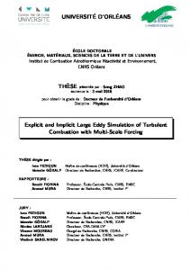
3. NUMERICAL TEST EXAMPLE AND RESULTS In this contribution the freezing of an infinite bar of Karlsruhe test substance with a rectangular cross section of 5 cm by 10 cm was considered. Although this application has no immediate practical evidence, it is convenient to highlight the properties of the different algorithms. The data of p(T), c(T) and k(T) were extracted from Fikiin [2]. A symmetric geometrical model was used and the finite element mesh consisted of 64 linear quadrilateral elements and 81 nodes (Figure 1). The initial and ambient temperatures TQ and Ta were set to 25°C and - 85°C, respectively. At the surface, an overall heat transfer coefficient hq of 15.9 Wm~2°C "l was assumed.

t ft tt tt t 30 00 20.00

■ * > !

10.00 0.00

"·

-1000

I ^s*-—

*h - · - - . ? - v .

\

-20.00

I

-30.00

T

'

-40.00

X

-50.00

t

-60 00

^.

-70.00 0.00

20.00

40.00

60.00

80.00

100.00 120.00

Urne I min I

r-

-node A - _ ^

node Β . · * .node C

A: centre node B: node between the centre and the boundary on the centre plane C: node at the boundary on the centre plane

Figure 5 Finite element mesh and time-temperature profiles at different locations For the solution of the non-linear system, Eqs(9-10) four explicit and seven implicit finite difference schemes were compared in terms of accuracy and CPU time: • Runge-Kutta (RK) methods of order 7 to 4 (7-step explicit methods) • Trapezoidal Rule (7-step of order 2 implicit method) • r-step Backward Differentiation (BDF) methods, r = 7 to 6 {order=r, implicit method). A mathematical description and discussion of these finite difference schemes can be found in Lambert [10]. The 6-step backward differentiation method with a time step of 0.1s and a relative error tolerance for h of 10~6 was used as reference method for comparing the accuracy of the several finite difference schemes. The accuracy was measured by means of the second norm of the error vector of the time-temperature profiles at the centre of the object. When implicit schemes were used the relative error tolerance for h was set to 10~4. The /--step BDF methods require r starting values. It is obvious that the initial condition is a first starting value. Other starting values are computed using the 7-step BDF method. In table 1 and 2 an overview is given of the accuracy and C PU time of the several explicit and implicit finite difference schemes as a function of the chosen time step for the solution of the non-linear system Eqs (9-10).

226

Table 2: Accuracy (°C) as a function of the time step Type EXPLICIT EXPLICIT EXPLICIT EXPLICIT IMPLICIT IMPLICIT IMPLICIT IMPLICIT IMPLICIT IMPLICIT IMPLICIT

Method 1st order RK 2nd order RK 3th order RK 4th order RK 1-step BDF 2-step BDF 3-step BDF 4-step BDF 5-step BDF 6-step BDF Trapezoidal Rule

dt=2s 6.0e-3 6.0e-3 6.0e-3 6.0e-3 2.0e-5 4.4e-6 3.3e-6 3.2e-6 3.4e-6 4.6e-6 2.5e-6

dt=4s unstable unstable 8.5e-3 8.5e-3 6.5e-4 1.5e-5 1.2e-5 1.3e-5 1.5e-5 3.0e-5 l.le-5

dt=10s unstable unstable unstable unstable 2.6e-3 9.0e-5 6.6e-5 8.7e-5 1.2e-4 2.0e-4 6.2e-5

dt=30s unstable unstable unstable unstable 1.3e-2 l.le-3 8.7e-4 l.le-3 1.3e-3 1.7e-3 4.0e-4

dt=60s unstable unstable unstable unstable 3.7e-2 5.5e-3 5.1e-3 6.2e-3 8.3e-3 1.2e-2 2.7e-3

dt=120s unstable unstable unstable unstable 1.0e-l 2.7e-2 2.7e-2 2.9e-2 3.4e-2 4.5e-2 6.7e-3

The Trapezoidal Rule is the most accurate finite difference scheme used in this work. The implicit methods are unconditionally stable which allow to use much larger time steps compared with the Runge-Kutta methods. Due to their very small stability regions, the use of explicit Runge-Kutta methods is highly restricted to the chosen time step. As a consequence, the time step should be considerable decreased to achieve the same accuracy as the implicit methods. Remark that for a given time step, the use of higher order BDF methods not results in a spectacular increase in accuracy. At the contrary, a decrease in CPU time is noticed. When using implicit schemes, each time step a non-linear algebraic system has to be solved in an iterative way. This iterative procedure is stopped when a user specified relative error tolerance for h is reached. The more severe this tolerance is chosen, the higher accuracy will be obtained. The use of higher order BDF methods requires less iteration steps to achieve a given tolerance, which results in lower CPU times. In terms of CPU time the low order Runge-Kutta methods are more attractive. From an accuracy and stability point of view their use is rather limited. Combining accuracy and CPU time, the implicit methods and the Trapezoidal Rule in particular are very powerful and most preferable. 4. CONCLUSIONS The simultaneous application of the enthalpy method and the Kirchhoff transformation is very convenient in solving complicated non-linear heat transfer problems, especially when phase changes have to be taken into account. The method is very elegant in a finite element framework as the non-linearities caused by the temperature dependent thermophysical properties are removed from the finite element system matrices. The constant properties and the sparse structure of the finite element system matrices can be exploited to develop very efficient and fast algorithms. The implicit finite difference schemes used in this work, for the integration of the differential system obtained from the finite element formulation, are unconditionally stable which allow to use much larger time steps compared with explicit methods. Although the explicit schemes are quite attractive in terms of computational effort, due to stability requirements their use is very limited. In terms of accuracy and CPU time the BDF methods and the Trapezoidal Rule in particular are very powerful.

227

Table 3: CPU time (s) as a function of the time step Type EXPLICIT EXPLICIT EXPLICIT EXPLICIT IMPLICIT IMPLICIT IMPLICIT IMPLICIT IMPLICIT IMPLICIT IMPLICIT

Method 1 st order RK 2nd order RK 3th order RK 4th order RK 1-stepBDF 2-steps BDF 3-steps BDF 4-steps BDF 5-steps BDF 6-steps BDF Trapezoidal Rule

dt=2s 539 880 1216 1561 1386 1363 1353 1362 1358 1361 1727

dt=4s unstable unstable 613 778 788 757 750 737 736 730 934

dt=10s unstable unstable unstable unstable 378 357 352 349 344 342 434

dt=30s unstable unstable unstable unstable 186 174 168 165 163 161 188

dt=60s unstable unstable unstable unstable 122 111 104 103 102 101 105

dt=120s unstable unstable unstable unstable 75 73 73 71 71 71 72

5. ACKNOWLEDG EMENTS The European Union (FAIR project CT96-1192 and PECO project CIPA CT93-0240) and the Flemish Minister of Science and Technology are gratefully acknowledged for financial support. Author Bart Nicolai' is Postdoctoral Fellow with the Flemish Fund for Scientific Research (F.W.O. Vlaanderen). 6. REFERENCES [1]

[2]

[3] [4]

[5]

[6] [7] [8]

[9]

Comini G., Nonino C. and Saro O. (1990) Performance of enthalpy-based algorithms for isothermal phase change. In: Advanced Computational Methods in Heat Transfer, Vol. 3: Phase Change and Combustion Simulation (Eds. Wrobel L.C., Brebbia C.A. and Nowak A.J.) Computational Mechanics Publications, Southampton Boston, 3-13. Fikiin K.A. (1996) Generalized numerical modelling of unsteady heat transfer during cooling and freezing using an improved enthalpy method and quasi-one-dimensional formulation. International Journal of Refrigeration, 19(2): 132-140. Anonymous (1993) Matlab-High Performance Numeric Computation and Visualization Software-User's G uide. The Math Works, Inc. Nicolai' B.M., Van den Broeck P., Schellekens M., De Roeck G., Martens T. and De Baerdemaeker J. (1995) Finite element analysis of heat conduction in lasagna during thermal processing. International Journal of Food Science and Technology 30(3):347-364 Scheerlinck N., Nicolai' Β.M., Verboven P. and De Baerdemaeker J. (1996) Finite element analysis of coupled heat and mass transfer problems with random field material properties. ASAE Annual International Meeting, Paper No. 963028, Phoenix, Arizona. Zienkiewicz O.C. and Taylor R.L. (1994) The Finite Element Method: Basic Formulation and Linear Problems, Volume 1. McGraw-hill Book Company Press W.H., Teukolsky S.A., Vetterling W.T. and Flannery B.P. (1993) Numerical Recipes in C, The Art of Scientific Computing, Volume 3. Cambridge University Press Saro O., Nonino C. and Comini G. (1995) An enthalpy-based algorithm for the analysis of phase change in nonhomogeneous media. In: Computational Modelling of Free and Moving Boundary Problems III (Eds Wrobel L.C., Sarler B. and Brebbia C.A.), Computational Mechanics Publications, Southampton Boston 127-134. Scheerlinck N., Fikiin K.A., Verboven P., De Baerdemaeker J. and Nicolai B.M. (1997) Numerical Solution of Phase Change Heat Transfer Problems with Moving

228

[10]

Boundaries using an Improved Finite Element Enthalpy Method. In: Computational Modelling of Free and Moving Boundary Problems IV (Eds Wrobel L.C., Sarler Β. and Brebbia CA.), Computational Mechanics Publications, Southampton Boston. Lambert J.D. (1991) Numerical Methods for Ordinary Differential Systems: The Initial Value Problem. John Wiley and Sons Ltd.

229

NOTICE TO THE READER Information on European Commi ssi on publi cati ons i n the areas of research and i nnovati on can be obtai ned from: ♦ CORDIS, the Community R & D Information Service For more information, contact: CORDIS Customer Service, B P 2373, L­1023 Luxembourg Tel. (352) 44 10 12­2240; fax (352) 44 10 12­2248; e­mail: [email protected] or visit the website at http://www.cordis.lu/

o Q

♦ Euroabstracts The European Commission's periodical on research publications, issued every two months. For more information, contact: RTD help desk, European Commission, DG XIII, L­2920 Luxembourg Fax (352) 43 01­32084; e­mail: rtd­[email protected]

Price (excluding VAT) in Luxembourg: ECU 26.50 * • * • _EUR_ •

OFFICE FOR OFFICIAL PUB LICATIONS OF THE EUROPEAN COMMUNITIES

• op • * • *

L­2985 Luxembourg

ISBN ΤΞ­ηΞη­33ϋΤ­7

co ω

O