Event Detection in Communication and Transportation Data

Event Detection in Communication and Transportation Data Joachim Neumann1 , Manqi Zhao2 , Alexandros Karatzoglou3 , and Nuria Oliver3 1

Jacoti Technologies, Barcelona, Spain [email protected] Google, Mountain View, USA [email protected] Telefonica Research, Barcelona, Spain [email protected], [email protected] 2

3

Abstract. The digitalization of the urban infrastructure and pervasiveness of mobile handsets allows to model the movement and communication patterns of people in the city. In this paper, we focus on automatically detecting unusual behavior (events) in the city of Barcelona by analyzing aggregated data from two urban sensors: cell phone towers and shared bicycle rentals. We use a state-of-the-art novelty detection algorithm and compare its performance to two alternative approaches. In addition, we design a simple tree classifier to distinguish between three types of unusual days: rainy days, holidays and days with special events.

1

Introduction

Our interactions in the physical world are increasingly leaving behind digital footprints. The analysis of these digital footprints by means of statistical tools and machine learning techniques has been coined Reality Mining [?]. The ultimate goal of reality mining techniques is to provide a deeper understanding about our lives, both at the individual and collective levels. Observing and modeling human behavior in urban environments is central to traffic forecasting [?], understanding the spread of biological viruses [?], designing location-based services, improving urban infrastructure and cellular network efficiency and detecting urban hotspots. A key difficulty faced by urban planners, virologists, and social scientists is that obtaining large, real-world observational data of human urban behavior is challenging and costly [?]. As websites have evolved to offer geo-located services, new sources of real-world behavioral data have begun to emerge. In addition, as city-wide urban infrastructures such as buses, subways, public utilities, and roads become digitized, other sources of real-world datasets that can be implicitly sensed are emerging. For example, recent work [?] has proposed a novel source of real-world human behavioral data from a new type of urban infrastructure: shared bicycling systems. They have successfully used bicycling station usage data to infer cultural and geographic aspects of the city and predict future station usage behavior, which corresponds to human movement in the city. Mobile phones play a key role as sensors of human behavior because they typically are owned by one individual that carries them at almost all times and are nearly ubiquitously used. While most of the previous work has focused on modeling typical human urban behavior, in this paper we turn our attention towards the automatic detection of interesting events or anomalous behavior at the city level and from two sources of digital footprints: shared bicycling and cell tower activity. Detecting atypical or novel events in an urban environment has several applications, including network management, traffic prediction and city planning. We analyze the value and limitations of two urban sensors that are part of the city infrastructure (shared bicycling and cell phone towers) and that provide partial information about the aggregated human behavior in the city. To the best of our knowledge, our work is the first to jointly analyze data obtained from these two types of urban sensors in order to detect and classify unusual behavior at the city level. Note that these large scale urban datasets tend to exhibit high levels of noise and periodic patterns. The term event is sometimes used in the time-series literature to refer to individual measurements (e.g., a call happening during a certain time of the day, a bicycle taken from a station at time t). In this work, however, we use the term event to refer to an activity that is unusual relative to normal patterns of behavior, such as unusually high or low phone call or bicycling activity. Hence, in our analysis we need to take into account both the patterns of typical and predictable behavior, along with the deviations from this behavior. This leads to one of the main challenges in event or anomaly detection: detecting anomalous periods of time requires some knowledge of what constitutes normal behavior. However, our datasets consist of both normal and anomalous (event) data mixed together without the availability of ground truth on what constitutes an event. Hence, the main contributions of this paper are:

2

– We propose a set of meaningful features that can be extracted from the two sources of real life input data: shared bicycling and cell tower activity; – We automatically detect anomalous urban behavior by adapting a state-of-the-art novelty detection approach to our datasets; – We propose a post-processing method to merge the events detected from each of the two urban sensors and automatically classify the detected anomalies into three types: weather, holidays and special events.

2

Related Work

Event detection can be regarded as one kind of anomaly or outlier detection. The survey paper [?] classifies the type of anomalies that can be detected into three categories: point, contextual and collective anomalies. If an individual data instance is considered to be an anomaly with respect to the rest of the data, then the instance is termed as a point anomaly. Unusual events in time-series, spatial or graph data are called contextual anomalies because each data point is composed of both the actual feature and its contextual attributes (e.g., time index, location information, graph topology, etc.). Finally, collective anomalies are a generalization of contextual anomalies where the goal is to detect a subsequence of a time-series, a local region of spatial data, or a subgraph as anomalous. Collective anomaly detection is generally the most challenging task of the three. In this paper we focus on anomaly detection from noisy spatio-temporal data and hence the problem that we tackle falls into the last category. A standart method that is often used for anomaly detection is the one-class Support Vector Machine (SVM) [?]. Event detection from spatio-temporal time series has been studied in the area of sensor networks. For example, Yin et al. [?] have recently proposed – and successfully applied to light sensor network data – a spatio-temporal event detection approach based on dynamic conditional random fields (DCRF), which handles the uncertainty of sensor data and allows neighborhood interactions [?]. Events are usually detected in sensor networks as a deviation from some constant background signal. These techniques cannot be easily applied to our problem because they typically assume that no pattern is recurrent in the sensor network. However, aggregate human urban behavior is often recurrent, particularly when each day’s measurement is taken as an independent data point. In [?], all the co-evolving sequences are modeled with a spatio-temporal moving average model whose parameters are estimated via standard regression. The estimation error is assumed to follow a Gaussian distribution and outliers/anomalies are detected when the measurement is two times the standard deviation away from the estimated value. This method is simple and efficient. However, the moving average model is assumed to be time-invariant and hence cannot capture the more general non-stationary processes that are found in our datasets. We shall highlight next the work by Ihler et al. [?] who use a model-based Markov chain Monte Carlo (MCMC) algorithm applied to freeway traffic data, which is assumed to be the superposition of a normal and an abnormal time series, both of which are modeled as Poisson counting processes. Moreover, there is a hidden state at each time instant which indicates the occurrence of event and the evolution of the hidden states are modeled as a two-state Markov process. The model parameters are estimated by means of the MCMC algorithm. Although this approach is certainly appealing, it would be difficult to directly apply it to our problem for several reasons: the model for freeway traffic data is very specific to the traffic problem and hence does not capture the potential events in datasets of different nature, such as ours. For example, in our shared bicycling dataset there are fewer bicycles on the road during rainy days but this kind of abnormality would not be captured by the MCMC model. In addition, the events at different time instants are all modeled to be Poisson random variables with the same parameter, which when applied to our noisy datasets would result in a high false alarm rate. Given the challenges and peculiarities of our datasets, we propose to use the general non-parametric adaptive anomaly detection algorithm proposed in [?], which is called localized p-value estimator (LPE). LPE is an efficient and provably optimal algorithm in the sense that it is uniformly most powerful for the specified false alarm level for the case that the anomaly density is a mixture of the nominal and any other density [?]. Another advantage of LPE is that it does not require the tuning of complex parameters and hence it is less sensitive than other approaches to the specific datasets.

3

Data

We analyze shared bicycling and cell phone activity data in the city of Barcelona (Spain) for 108 full weekdays, from September 1, 2009 to March 15, 2010. We had to exclude Sep. 16 to Sep. 30, 2009, Nov. 9, 2010, Nov.

3

11 to Nov. 30, 2010 and Feb. 26, 2010 because of limited access to cell phone call records. We focus our analysis on weekdays, excluding Saturdays and Sundays, because behavioral patterns typically show larger variation during weekends. We shall describe next the two datasets that are the object of our study. 3.1

The Shared Bicycle Dataset

Barcelona’s shared bicycle program, Bicing, was launched in March of 2007 and has currently about 400 stations and 115,000 subscribers. Bicycles are checked out by swiping an RFID membership card at a Bicing station kiosk, which unlocks bicycles and displays their rack location on an LCD screen. Bicing is open from 5AM to 12AM on Sunday through Thursday and 24 hours during the weekend. The Bicing website reports the status of all bicycle stations via a Google Maps visualization. We scrape this webpage every two minutes and extract three data elements per station: the station’s geo-location, the number of available bicycles and the number of vacant parking slots, based on which the percentage of availability can be derived. This dataset can be regarded as a spatial-temporal process. The data scraped from the Bicing website is noisy due to temporary station closures, maintenance work, connectivity failures, web site time-outs, etc. Hence, we employ the three-step data cleansing method that is described in [?] and [?] to detect and eliminate faulty observations. Feature extraction We compute the shared bicycling activity feature vector as follows: For each of the 390 stations that produced valid data during the period of interest, we calculate the absolute difference between two consecutive observations and average this difference in one-hour bins. Suppose the 30 original measurements – we obtain one measurement every 2 minutes – in a one-hour bin are N1 , · · · , N30 . Then the P29 hourly activity is defined as i=0 |Ni − Ni+1 |. The median of the hourly activity of all stations is calculated and normalized to values between 0 and 100 to yield the aggregated Bicing daily activity feature vector of length 24, one entry per hour (see Figure ??). 3.2

The Cell Phone Dataset

Call Detail Records (CDRs) are generated when a cell phone that is connected to a mobile phone network makes or receives a phone call or uses a service (e.g., SMS, MMS, etc.). For invoice purposes, this information is logged together with the cell tower ID which gives an indication of the geographical position of the user. We analyze the anonymized CDRs for one cell phone operator in the city of Barcelona and during the time period of study. Feature extraction We analyze a total of about 324 million phone calls and SMS messages in Barcelona in the period between from Sep. 1 and Mar. 15, 2010. In order to yield a dataset that is comparable to the aggregated Bicing activity, we extract the total number of SMS/MMS and calls that were made/received per hour in the 1392 cell towers that are inside the area that is covered by Barcelona’s shared bicycling system. Again, a normalization to [0, 100] is applied to calculate the daily cell phone activity feature vector of length 24. 3.3

Ground Truth Data

We extract two types of ground truth data: Firstly, we identify holidays from an official calendar from the city of Barcelona. Our event detection algorithm will point us to days that are not in this calendar, although these are perceived by some as holidays, e.g. December 24, or long weekends on which many Spaniards do not go to work (e.g., a Monday that is followed by a holiday). However, these days are not part of the ground truth of holidays; Secondly, we detect days with a daily precipitation ≥ 1 mm. This data suffers from a lack of spatial precision: we have only the data from Barcelona’s airport4 while precipitation in Barcelona could be locally confined. Rain is an interesting phenomenon since it affects the usage of the Bicing system while the number of cell phone calls is probably unaffected. 4

from http://www.wunderground.com

4

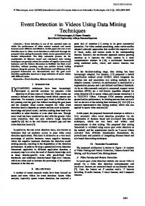
Fig. 1. Normal vs. Anomalous days: Example of aggregated normalized activity as a function of the hour for March 10, 2010 (normal day, solid line) and March 08, 2010 (anomalous day due to snow, dashed line). Bicing activity is shown in blue and cell phone activity in red. In the anomalous day, the Bicing activity decreases while the cell phone activity increases when compared to a normal day.

4

Event Detection Algorithm

Assume a training set S = {x1 , x2 , · · · , xn } and xn+1 as a test point, where in our case each point xi is a feature vector of length 24 (as previously explained). Since the activity feature vectors from both datasets have the same format, we treat them exactly the same way in the event detection stage. We will later merge the event detection results. The Localized p-value Estimator (LPE, [?]) method can be summarized as follows. First we calculate the pairwise Euclidean distances dij = kxi − xj k2 between all the points in order to form a K-nearest neighbor graph (K-NNG) by connecting each xi to the K closest points {xi1 , · · · , xiK } in S − {xi }. Note here that any distance measure d can be used instead of the Euclidian distance. We then sort the K-nearest distances for each xi in increasing order di,i1 ≤ · · · ≤ di,iK and denote RS (xi ) := di,iK , that is, the distance from xi to its K-th nearest neighbor. The LPE score function: n

pˆK (xn+1 ) =

1X I{RS (xn+1 )≤RS (xi ))} n i=1

(1)

maps the test data xn+1 to the interval [0, 1], where I{·} is the indicator function. Finally, a test point xn+1 is declared to be an “anomaly/event” at a pre-defined significance level α, if pˆK (xn+1 ) ≤ α. It is proven in [?] that asymptotically the empirical false alarm rate for LPE converges to α and the mis-detection rate is minimized under the significance level α. In real applications, the nominal training set is always acquired via human labeling. Acquiring this information is often time-consuming and - as in the case of special events - badly defined or even impossible. Interestingly, even under the unsupervised learning setup where we don’t know whether the element in S = {x1 , x2 , · · · , xn } is normal or not, the above LPE algorithm can still be applied. However, in this case, the pre-defined significance level α no longer reflects the empirical false alarm, but it becomes a parameter which reflects the percentage of anomalies that we expect in the dataset. A crucial factor in the LPE algorithm is the choice of the distance metric d(xi , xj ). In our application, since we already make our detection robust by binning the data to create the feature vector, the simple Euclidean distance yields to good performance. Start and end of the event: Since the feature vector represents a time-series, we are also interested in the start time and end time of events. For this purpose, we apply the following simple yet effective thresholdingbased method to the days that have been identified as “anomaly/event”:

5

1. Compute the difference D between the feature vector of the event day and the average feature vector among all days; 2. Pick up a threshold β; 3. Initialize with start = 1 and end = 24; 4. Repeat until end − start = 1 or no further change is made: (a) If |D(start)| ≤ β, increase by 1; (b) If |D(end)| ≤ β, decrease by 1; 5. Output: start and end; We use the start/end information to determine the duration of the event in the event classification step (see Section ??). 4.1

Evaluation of the Event Detection Algorithm

In this section, we compare our localized p-value estimation algorithm (LPE) to two alternative algorithms: the popular one-class Support Vector Machine (OCSVM) and a difference thresholding algorithm (DIFF). The DIFF method is a simple thresholding-based algorithm, in which we compute the difference between each day’s value and the average, then calculate the `1 norm of this difference vector (i.e., the total absolute difference) and finally compare this value to a threshold to declare the event. These three approaches contain tuning parameters which explicitly or implicitly control the number of detected events. For the performance comparison, we use only the Bicing dataset, because this allows us to use both holidays and rainy days as ground truth (cell phone activity is not as significantly affected by rain as bicycling is). The use of the Bicing data also allows us to utilize a larger dataset in this comparative analysis: We use 245 weekdays between August 31st 2009 and August 6th 2010 for which we have a total of about 68 million observations. In this period, we identify a total of 115 days with ground truth events: 19 holidays and 102 rainy days of which 6 overlap. Note that we are interested in minimizing the false positive rate of the algorithms in order to make sure that all detected events are real events. We therefore settled on parameter settings of the three algorithms that yields 44 detected events. The false positive rate of the algorithms increased significantly with a larger number of events, hence lowering the overall confidence on the event detection system. We understand that this is a limitation of our evaluation methodology. Also note that there is a certain level of noise in our ground truth: a few of the days that were labeled as rainy had minimal precipitation in the city of Barcelona. We therefore consider the precision of the algorithms to be more important than their recall. We adjust the parameters of all three algorithms so that they detect the exact same number of events (44) in the Bicing dataset. We adjust the parameter of the LPE algorithm to yield a maximum number of detected events while avoiding false positive detections. We then tune the parameters of the OCSVM and DIFF algorithms to yield the same number of detected events. Table ?? shows the performance of the three algorithms. Based on this, we compute the precision, recall and F1 measures, see Figure ??. Quite surprisingly, the DIFF algorithm, though simple and naive, still does a much better job than the more sophisticated the OCSVM algorithm. This phenomenon might be ascribed to the fact that OCSVM is not very robust to a highly noisy dataset such ours. We also observe that LPE clearly outperforms both OCSVM and DIFF in terms of F1, recall and precision. While we fix the precision of the LPE algorithm, its recall rate outperforms that of OCSV and DIFF. Note that the task of event detection with real-life data is inherently hard, since the definition of what constitutes an event can be ambiguous. The evaluation will thus not reflect the exact performance of the algorithms since it is very difficult to define objective ground truth, i.e., although we have information about precipitation in Barcelona we do not know whether it was strong enough to actually affect the Bicing usage. The evaluation should thus be regarded as an indication of the level of performance of the algorithms rather than a hard proof.

5

Event classification

We ran the LPE event detection algorithm on the 108 weekdays for which we had data from both data sources (Bicing and cell phone activity). After pre-processing and for each data source, we created 108 (for

6 LPE event non event detected event 44 0 detected non event 71 (3) 130 OCSVM event non event detected event 30 14 detected non event 85 (3) 116 DIFF event non event detected event 37 7 detected non event 78 (8) 123 Table 1. 2x2 frequency tables for the three methods for the 115 event days and 130 non event days. The false negatives contain a large number of rainy days: the false negatives that are holidays are given in parenthesis.

Fig. 2. Precision, recall and F1 measure for the three event detection algorithms. LPE clearly outperforms OCSVM and DIFF

each day) 24-dimensional feature vectors and used identical parameters for the event detection on both datasets. In these datasets, our algorithm detected a total of 32 events, where 29 events were found in the Bicing dataset and 18 events in the cell phone dataset (15 events were detected in both datasets). We also compute the duration of each event as the difference between its start and end points (see Section ??). We now present a simple algorithm to automatically classify these events. We are interested in classifying the type of event into three classes: rainy days, holidays and special events. The latter are days that are neither holidays nor rainy days, but that are detected as events. To this end, we employ a simple classification tree where the event is characterized by its intensity, given by the Euclidean distance to the median pattern, and its duration. The intensity and duration of all detected events (in either Bicing or cell phone data) is given as input to the tree in order to classify the type of the event. The resulting tree is depicted in Figure ??. We observe that weather events can be easily picked up by the fact that the cell phone call activity remains unchanged while the Bicing activity changes (the Bicing activity actually drops consistently, but this information was not needed in our event classification). For days where both call and Bicing usage behavior are unusual, the call behavior deviation makes the difference: if less-than-average calls were made, its a holiday while special events are characterized by more phone calls. Of particular interest are the days that fell in the category of special events, because these were unusual days that were discovered by the algorithm and for which we did not have an a priori explanation. We took a deeper look at what made such days peculiar and asked several locals for possible explanations. Their consensus is listed in Table ??. Interestingly, we were able to find a convincing explanation for all of these days. The relative increase or decrease of cell phone activity corresponds to the interpretation of these days as special events (more activity) or holidays (less activity). Note how the days before Christmas were detected as special events with an increased CDR activity while the first weekday after Christmas showed (as the holidays themselves) a decreased CDR activity. This qualitative method is of course inherently blind to events that our algorithm failed to detect (false negatives).

7

Fig. 3. Classification tree of the event types based on the CDR and Bicing events and the level of activity.

Surprisingly, there were a few days (e.g. Easter Monday) that – contrary to our expectation – were not discovered by our algorithm because they did not appear to significantly differ from the city’s usual behavior. In addition to discovering unusual behavior (events) from these type of real-life data, our algorithm characterizes each event in terms of its intensity and duration. Therefore, we are able to quantify the impact that various contextual factors (e.g., rain, holidays...) have on the city’s aggregated behavior (as perceived by the shared bicycling and cell phone activity sensors). In this regard, we found that special events like unusual amounts of snow had the largest impact on the city’s behavior, followed by holidays.

Activity Date in CDR Description 14.09 2009 more First day of school. At 2pm kids leave school 22.10 2009 more Unusual heavy rains, major public transport problems 07.12 2009 less Unofficial holiday between a Sunday and a holiday 18.12 to 24.12 2009 more Before Christmas, shopping activity 28.12 2009 less After Christmas, unofficial holiday 08.03 2010 more A lot of snow, Barcelona collapses 09.03 2010 more Day after the heavy snow public transport problems Table 2. Complete list of all days for which the CDR data has been classified as event. The consensus of possible explanations from several locals from Barcelona is given for each event

6

Conclusions

In this paper, we have shown the feasibility of an automatic event detection algorithm (LPE) applied to data from two urban sensors: shared bicycling and cell phone activity. The use of these two datasets of different nature allows us to detect more events and to characterize the event type. Moreover we show that the LPE algorithm outperforms OCVSM and DIFF in terms of event detection and shows good precision characteristics.

8

In future work, we plan to explore the impact of deviations in temporal activity patterns for more fine grained event classification. We are also interested in jointly analyzing the data from these two urban sensors at the feature level rather than at the decision level. Better spatial granularity would enable us to detect locally confined events. For this purpose, we are working on a clustering algorithm that joins stations and cell towers with similar behavior. Finally, we would like to design an online extension of LPE to allow for real-time event detection.

7

Acknowledgements

This work is funded as part of a Marie Curie Intra European Fellowship for Career Development (IEF) award (CARS, PIEF-GA-2010-273739) held by Alexandros Karatzoglou.

References 1. N. Eagle and A. S. Pentland, “Reality mining: sensing complex social systems,” Personal Ubiquitous Comput., vol. 10, no. 4, pp. 255–268, 2006. 2. E. Horvitz, J. Apacible, R. Sarin, and L. Liao, “Prediction, expectation, and surprise: Methods, designs, and study of a deployed traffic forecasting service,” in Proceed. IUI 05, July 2005. 3. L. S. Tsimring and R. Huerta, “Modeling of contact tracing in social networks,” Physica A, vol. 325, pp. 33–39, 2003. 4. D. D. Brockmann, L. Hufnagel, and T. Geisel, “The scaling laws of human travel,” Nature, vol. 439, pp. 462–465, 2006. 5. J. Froehlich, J. Neumann, and N. Oliver, “Prediction, expectation, and surprise: Methods, designs, and study of a deployed traffic forecasting service,” in Proceed. IUI 05, July 2005. 6. V. Chandola, A. Banerjee, and V. Kumar, “Anomaly detection: A survey,” ACM Comput. Surv., vol. 41, no. 3, pp. 1–58, 2009. 7. B. Sch¨ olkopf, J. C. Platt, J. C. Shawe-Taylor, A. J. Smola, and R. C. Williamson, “Estimating the support of a high-dimensional distribution,” Neural Computation, vol. 13, pp. 1443–1471, July 2001. 8. J. Yin, D. H. Hu, and Q. Yang, “Spatio-temporal event detection using dynamic conditional random fields,” in Proceedings of the Twenty-First International Joint Conference on Artificial Intelligence (IJCAI 2009), Pasadena, California, USA, 2009, pp. 1715–1720. 9. B.-K. Yi, N. D. Sidiropoulos, T. Johnson, H. V. Jagadish, C. Faloutsos, and A. Biliris, “Online data mining for coevolving time sequences,” in Proceedings of the 16th International Conference on Data Engineering, Washington, DC, USA, 2000. 10. A. Ihler, J. Hutchins, and P. Smyth, “Adaptive event detection with time-varying Poisson processes,” in Proceedings of the 12th ACM SIGKDD international conference on Knowledge discovery and data mining, New York, NY, USA, 2006, pp. 207–216. 11. M. Zhao and V. Saligrama, “Anomaly detection with score functions based on nearest neighbor graphs,” in Neural Information Processing Systems Conference, vol. 22, 2009. 12. J. Froehlich, J. Neumann, and N. Oliver, “Measuring the pulse of the city through shared bicycle programs,” in International Workshop on Urban, Community, and Social Applications of Networked Sensing Systems - UrbanSense08, Raleigh, North Carolina, USA, November 4 2008.