Evolving a Bayesian Classifier for ECG-based Age Classification in Medical Applications M. Wiggins* 1a, A. Saad*2 a, B. Litt3, and G. Vachtsevanos* *School of Electrical and Computer Engineering Georgia Institute of Tec hnology 1 Atlanta, GA 30332, USA 2 Savannah, GA 31407, USA 3 Departments of Neurology and Bioengineering, University of Pennsylvania, Philadelphia, PA 19104, USA
Abstract. Objective: Age classification of patients based on information extracted from electrocardiograms (ECG’s). The scope of this work is to develop and compare the performance of Bayesian classifiers. Methods and Material: We present a medical patient classification methodology using a genetically evolved Bayesian network classifier and biological signal characteristics. Patient age classific ation is performed based on statistical features extracted from electrocardiogram signals. The continuous signal feature variables are converted to a discrete symbolic form based on thresholding to lower the dimensionality of the signal allowing for smaller conditional probability tables to be calculated for the classifier. Two methods of network discovery from data were developed and compared: the first using a greedy hill-climb search and the second method based on evolutionary computing using a genetic algorithm (GA). Results and Conclusions: Performance of both Bayesian network discovery methods was measured using the area under the receiver operating characteristic (ROC) curve and compared to the performance of a naive Bayesian classifier. The evolved Bayesian network performed better (86.25% AUC) than both the one developed using the greedy algorithm (65% AUC) and the naïve Bayesian classifier (84.75% AUC). The methodology for evolving the Bayesian classifier can be used to evolve Bayes ian netw orks in general thereby identifying the dependencies among the variables of interest. Those dependencies are assumed to be non-existent by naïve Bayesian classifiers. Such a classifier can then be used for medical applications for diagnosis and prediction purposes. Keywords: evolved bayesian classifier; ECG-based age classification; hybrid soft computing techniques.
1. Introduction
4
QRS
3.5 3 Voltage (mV)
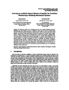
The human heart is a complex system that gives many clues about its condition in its electrocardiogram (ECG) signal (Figure 1). Trained physicians are able to recognize certain patterns in a patient's ECG signal and use them as the basis for diagnosis [1], for instance to diagnose heart ailments such as arrhythmia (using the QRS complex) [2], ischemia [3, 4], or prediction of an impending heart attack (acute myocardial infarction) [5]. Researchers have tried since the inception of computers (e.g., see [6, 7]) to develop techniques and algorithms for automated processing of ECG signals for various medical applications, whether as standalone applications or as a
2.5 2
P
1.5
T
1 0.5 0 -0.5 0
0.2
0.4
0.6 Time (s)
0.8
1
Figure 1. Electrocardiogram (ECG) Signal with the QRS complex, a Email addresses for correspondence authors:
[email protected] and
[email protected]. P- and T -waves indicated.
1
decision aid to physicians. However, patterns of an ECG signal are difficult to discern due to the multitude of characteristics that are embedded in the signal. As a result, researchers have focused on developing specific techniques to extract information from ECG’s for specific applic ations. This paper demonstrates the applicability of evolving a Bayesian Network (BN) classifier to distinguish between two groups of individuals based on ECG features derived from young and elderly, healthy adults, hereby referred to as young and elderly patient groups, respectively. If this method can distinguish between the two patient groups, a more complex classification problem, such as cardiac disease risk stratification might be attempted, with the potential of yielding better accuracy than traditional methods for fusing multiple clinical measurements. With heart disease being the biggest killer in America and a billion dollars spent each year on Atrial Fibrillation following Coronary Bypass Surgery [8], there is a wealth of classification and risk stratification problems to be addressed. This motivates a thorough investigation of classification of patient risk, through the use of biological heart signals and other patient data. The remainder of the paper is structured as follows: section 2 gives an overview of techniques and algorithms for processing ECG signals in medical applications, with a focus on applications involving classification; section 3 presents an overview of ECG signal processing, including the techniques used in this study; section 4 presents an overview of network structure discovery techniques, including the two techniques used to develop the Bayesian classifier; section 5 presents the results; section 6 presents a discussion; and section 7 concludes the paper and presents directions for future work.
2. ECG Signal Processing In order to identify the behavioral characteristics of an ECG, numerical quantifications are needed to decompose the signal into components that can be analyzed using computerized means. While many types of quantifications can be derived – referred to as signal features herein – it is often difficult to combine and assess them in meaningful and useful ways for a given application. For instance, an algorithm for detecting the QRS complex in an ECG has been reported in [9], a framework for the classification of the 12-lead ECG has been presented in [10], and an interactive framework for analyzing ECG signals has been proposed in [11]. In a clinical study, Chandy et al. collected both pre- and postoperative surface ECG signals from 300 patients undergoing coronary artery bypass graft (CABG) in order to identify differences in ECG P wave morphology, which could distinguish Atrial Fibrillation developing patients from normal patients [12]. In another study, detection of ventricular tachycardia and fibrillation by using an ECG symbolic conversion and complexity measurement was done with 100% accuracy for a large test set in [13]. Two main approaches for biological signal processing exist today. The first is the sliding window method, which involves segmentation of the data into smaller lengths. These segments are usually uniformly spaced within the original signal and may or may not have overlapping points with other windows. A feature or statistical measure is calculated for each segment, such as frequency content or signal amplitude standard deviation. Each of these calculations can then be placed in temporal order according to its location in the original signal, forming a representation of that feature’s progression through time over all windows. This compressed signal representation may be useful when looking for a change of state leading to a physiological event, such as determining the onset of a seizure from brain waves or a heart attack from ECG’s. When no significant signal or state changes are expected, the sliding window method does not hold as much promise. For this reason, the second method of biological signal feature calculation is simply feature calculation over the entire signal, as if the window in the first method was set as the entire available signal. While some variations in the signal’s characteristics might not be identified, an overall signal characteristic is obtained in a single numeric value. There are clearly a multitude of features, transformations, and statistics that can be applied to an ECG signal, including wavelet, frequency, and nonlinear transforms with statistical, temporal, and
Figure 2. Feature Extraction Block Diagram
2
Voltage (mV)
4 3 2 1 0 0
0.5
1
1.5
2
2.5
3
3.5
2.5
3
3.5
Voltage (mV)
Time (s)
2 1.5 1 0.5 0 -0.5 0
0.5
1
1.5
2
Time (s)
Figure 3. Original ECG signal (top) and ECG signal (bottom) after preprocessing by low -pass and high -pass filters.
chaotic feature extraction performed on them. While discovery of hidden patterns or subtle deviations in the signal shape or other properties are the main objectives of these labors, other purposes include compression [14, 15], coding [16], or detecting characteristic points [17] of ECG signals. For the purposes of this study, statistical features were calculated over the entire period of ECG’s obtained from a medical database. Figure 2 depicts the block diagram of the signal processing that was performed in this study. Data used for this study was obtained from the Fantasia database (available on www.physionet.org [18]). The database consists of ECG’s from twenty 21-34 and twenty 68-85 yearold subjects, hereby referred to as young and elderly patient groups, respectively. These patients were rigorously screened for any preexisting heart conditions and all were considered to be normal, healthy individuals. They underwent supine resting while continuous ECG was collected for 120 minutes at a sampling rate of 250 Hz. Each subgroup of subjects comprised an equal number of men and women. The data was imported into Matlab (Release 13) for computation. Preprocessing consisted of highpass filtering with a 4th order Butterworth filter with a cutoff of 0.004 Hz; done to remove the baseline drift DC voltage that sometimes builds on ECG electrodes [9]. A low pass 5th order butterworth filter with cut-off frequency at 20 Hz was used to remove noise as well as smooth the shape of the signal without loss of significant cardiac information content. Figure 3 shows a patient’s ECG signal prior to preprocessing (top) and after (bottom). 2.1. ECG Signal Feature Extraction The 120-minute signals were then used to calculate the feature set, F, comprising the 12 feature measures listed in Figure 4. The rationale for choosing th ese features is based on insights and bac kground in signal processing, as follows. The energy and the 4th power of the signal can show the signal’s tendency to stay either above or below the baseline, closely related to the signal’s integral. The nonlinear energy, known as the Teager energy in [19], includes amplitude and instantaneous frequency information, along with the energy component. Shannon entropy is a measure of the randomness of the amplitude values of the signal [20]. The higher the entropy, the more disordered and closer the signal is to random Brownian motion. Frequency domain based features can reveal other important characteristics of the signal [21]. The peak frequency and peak power identify at what frequency the signal oscillates with the most power and the magnitude of this power peak, respectively. The mean and median frequency features reveal the frequency value in the power spectrum where the mean and median frequencies appear, respectively. Spectral entropy is a measure of the regularity of the power spectrum of the signal [19]. This feature can give an indication of the overall frequency distribution, while the above frequency characteristics do not. Both Katz fractal dimension and the Hurst
3
parameter are measurements of the long-range dependence of the signal. These measurements can identify if a signal is becoming non-stationary, increasing in complexity, or changing its space filling properties. Most importantly, they show the signal’s self-similarity. This property can be very useful when looking for repetitions that may not be obvious to a human observer. The feature curve length tends to correlate with the above features closely, also showing the space filling property without as much sensitivity to the self-similarity measure [19]. Given the inherent variability in ECG signals among patients, each of these features offers information that can be used to distinguish between patient classes. We believe that, collectively, these features can help distinguish the two classes. The extraction of feature values from the ECG signals reduces the dimensionality of the problem to a computationally tractable level. In this process, signal information is encoded so that it can be used for classification or prediction.
Energy = ∑ xi
PeakPower = max( PSD )
2
4th Power = ∑ xi
PeakFrequency = index(max( PSD ))
4
NonlinearEnergy = ∑ −xi ⋅ xi −2 + xi2−1
CurveLength = ∑ xi − xi−1
SpectralEntropy = ∑ PSD ⋅ log( PSD )
range ( xi ) i Hurst = ln − 2 std ( xi ) KatzFractalDimension =
MeanFrequency = index( mean( PSD )) MedianFrequency = index( median( PSD )) ShannonEntropy = −∑ hist ( x) ⋅ log( hist ( x ))
k
∑
i =1
l o g ( k − 1) 2 max( ∑i ( x i − x1 ) + i 2 log 2 ∑i ( x i +1 − x i ) + 1
) + l o g ( k − 1)
Figure 4. Equations of the features in F, calculated on the ECG signals.
After extraction, feature values are discretized into binary form based on their value being above or below a certain threshold. This threshold was set using a Receiver Operating Characteristic (ROC) curve, where a feature value is predictive of the variable of interest, in this case, age.
Figure 5. ROC curve (left) created to determine the classification threshold set as the maximum of the product of the sensitivity and specificity plot (right). The diamonds represent patients from the elderly age group, while the circles represent those in the young age group. The vertical line represents the determined feature value threshold for the shown feature, peak frequency.
A location on the feature value continuum slightly greater than the maximum of the product of the sensitivity and the specificity is used as the threshold. This threshold determination is depicted in Figure 5, showing the ROC on the left and the product of sensitivity and specificity on the right. Diamonds represent elderly patients and circles represent young patients, while the vertical line shows the chosen threshold for binary discretization. This threshold is different for each of the 12 features, based on the best sep aration for that feature’s values. This technique culminates in class and feature infor-
4
mation needed to train a classifier, for instance, allowing for the computation of conditional probability tables needed to build a Bayesian Network classifier, as explained in the following sections.
3. Bayesian Network Structure Discovery A conditional probability is the likelihood of some conclusion, C, given some evidence/observation, E, where a dependence relationship exists between C and E. This probability is denoted as P (C | E ) where
P(C | E) =
P( E | C ) ⋅ P (C ) P( E)
(1)
Bayes’ theorem is the method of finding the converse probability of the conditional,
P( E | C) =
P(C | E) ⋅ P ( E ) P( C, E ) = P (C ) P(C )
(2)
This conditional relationship allows an investigator to gain probability information about either C or E with the known outcome of the other. Now consider a complex problem with n binary variables, where the relationships among them are not clear for predicting a single class output variable (e.g., node 1 in Figure 6). If all variables were related using a single joint distribution, the equivalent of all nodes being first level parents, the number of possible combinations of variables would be equal to (2n-1). For each combination, a sufficient number of samples must occur to obtain a realistic likelihood estimate. This results in the need for a very large amount of data [22, 23]. If dependence relationships between these variables could be determined resulting in independent variables being removed, fewer nodes would be adjacent to the node of interest. This parent-node removal leads to a significant reduction in the number of variable combinations, thereby reducing the amount of needed data. Furthermore, variables that are directly conditional, not to the node of interest but to the parents of the node of interest (as nodes 4 and 5 are with respect to node 1 in Figure 6), can be related, which allows for a more robust system when dealing with missing data points. This property of requiring less information based on pre-existing understanding of the system’s variable dependencies is a major benefit of Bayesian Networks [23]. Some further theoretical underpinnings of the Bayesian approach for classification have been addressed in [24] and [25].
Figure 6. Basic Bayesian Network Structure and Terminology
A Bayesian Network (BN) is a relatively new tool that identifies probabilistic correlations in order to make predictions or assessments of class membership. The first BN’s were created with expert knowledge and usually dealt with fairly well understood principles and variable relationships. Currently, many complex problems exist where a researcher may ha ve ample data for the variables of interest, but does not know the relationships between those variables in order to create the network. As mentioned previously, as the number of parents grows, the amount of data required to derive a conditional probabilit y table of the BN grows exponentially. Therefore, the number of possible parents is limited by the size of the data set available. Besides the data requirement, the network must be built in
5
a computationally viable way, while still producing accurate conditional variable dependencies [22, 23, 26]. For this study, two methods of network discovery were developed and compared: the first using a greedy hill-climb search and the second method based on evolutionary computing using a genetic algorithm. Performance of both methods was measured and compared to the classification accuracy obtained by a naive Bayesian classifier.
3.1. Naïve Bayesian Classifier Given an evidence set E = {E 1,E 2, …, En}, the joint probability in the numerator of Equation. (2), P ( C , E ), can be expanded using the definition of conditional probability to P (C , E1 ,..., En ) = P(C ) ⋅ P( E1 ,..., En | C ) = P(C ) ⋅ P( E1 | C )⋅ P(E2 ,... En | C ,E1 )
(3)
= P(C ) ⋅ P( E1 | C ) ⋅ P( E2 | C, E 1) ⋅ P( E3 ,...En | C , E1 ,E2 ) = P(C ) ⋅ P( E1 | C )⋅ P( E2 | C , E1 )⋅ P( E3 | C , E1 , E2 ) ⋅ P( E4 ,...En | C ,E1 ,E2 ,E3 )
and continuing. This expansion requires the use of significant amounts of data to determine the many probabilities. In order to reduce the num ber of required data samples, an assumption of independence can be made for the components of E, letting the joint probability take the form of
P( C, E1 ,..., En ) = P(C ) ⋅ P( E1 | C) ⋅ P( E2| C) ⋅ P( E3| C) L ,
(4)
n
= P(C )∏ P ( Ei | C) i =1
The use of this independence assumption is at the basis of the “naïve” Bayesian classifier. A network is created with only one node representing the class of interest and all other nodes as its 1st level parents. The joint probability of the node of interest is then computed as in Equation. (4). While the independence assumption may seem as a simplifying one and would therefore lead to less accurate classification, this has not been true in many applications. For instance, several datasets are classified in [27] using the naïve Bayesian classifier, decision tree induction, instance-based learning, and rule induction. These methods are compared showing the naïve classifier as the overall best method. To use a Bayesian Network as a classifier, first, one must assume that data correlation is equiv alent to statistical dependence. Though this is not true from a pure mathematical standpoint, for purposes of medical diagnosis when no dependencies can be determined with a high degree of certainty, correlation between the two variables is assumed to give similar information. We also must assume that the data gathered accurately portrays the system, and with small datasets, this can be a difficult idea to accept or cross validate.
3.2. K2 Algorithm Researchers have proposed various techniques for BN structure discovery without the above independence assumption, the most notable being Cooper and Herskovits, who developed the K2 algorithm, a greedy-hill climb algorithm [23]. This method starts with a graph and repetitively adds nodes/edges to maximize the following model-selection crit erion,
Γ
q
K 2 criterion = ∏ j =1
Γ
(∑
(∑
k
aijk
)
a + ∑ k sijk k ijk
6
ri
)
∏ k =1
Γ ( aijk + sijk ) Γ ( aijk )
,
(5)
where • i, j, and k are the indexes of the child node, of the parents of the child node, and of the possible values of the child node, respectively, • q is the number of different instantiations of parent nodes, • ri is the number of values that the child node can assume, • s is the number of times that the child node has the value of the k th index value of the node, and • a is the number of times that the parents and the child correlate pos itively in discrete cases. This selection criterion is basically a measure of how well the given graph correlates to the data. This method requires a complete dataset without any missing data points and a hierarchical causal ordering of nodes. This means that the nodes are listed so that any node preceding a given node can be its parent, while those following it cannot [22, 23, 26]. As a greedy-hill climb algorithm, the K2 algorithm suffers from a major limitation: it can terminate the search after encountering the first local maximum without finding the overall global maximum. Several methods for random restarts, such as simulated annealing and best-first search, have been proposed to eliminate this problem. Nonetheless, these methods are more computationally expensive, but in many cases, can still improve the network’s accuracy when dealing with large data sets [22].
3.3. GA for Network Structure Discovery A Genetic algorithm (GA) is another tool that can be used to discover the Bayesian network structure. The general GA-evolved BN algorithm framework is shown in Figure 7. The algorithm can be designed to begin with an initial BN structure population and then assesses fitness of these structures. Iteratively, random crossovers and mutations of networks within a population are tested, and the most fit of the population is kept for future generations. As generations pass, the population evolves leaving the fitter structures, while those performing poorly are discarded. This method is quite useful due to the inherent randomness that alleviates the local maximum problem as seen in the K2 algorithm. An improvement is also gained since the structure of the resulting network is dynamic without regard to individual node-to-node fitness measures that have not been proven to be optimum or accurate [26]. These method characteristics allow intelligent model construction without requiring an ex haustive search of all possible structure combinations of nodes.
Figure 7. Block Diagram of Genetic Algorithm Structure Discovery of Bayesian Networks.
7
4. Method We developed a total of four Bayesian classifiers: two using the naïve Bayesian approach, assuming conditional independence of all features, and two classifiers where the conditional dependencies between features are to be determined using structure discovery methods. The first of the two naïve Bayesian classifiers was built using all twelve features for classification and the second using a subset of the features. The first of the two methods for network structure discovery is based on the K2 algorithm (described in section 3.2), and the second is based on evolutionary computation us ing a genetic algorithm. Typically, the set of nodes presented in section 3.2 is causally ordered, before the algorithm begins structure discovery. The main benefit of this order is reducing the search space of possible node-tonode connections. With a set comprising only 12 nodes, this would produce relatively little computational benefits. Also, with this data set, where features do not have a truly casual relationship, any ordering would not be beneficial, and might even hinder the network discovery by ruling out possible solutions. The network discovery methods begin with the full set of nodes with no edges between them. When a greedy algorithm is used, the utility of adding an edge between any two nodes is assessed and the edge with the maximum scoring utility is chosen and added. In the work reported herein, the score for adding nodes to the network was calculated using the Cooper-Herskovits scoring criterion given in Equation (5) [22, 23, 26]. The second BN structure discovery method implemented uses a GA. The variables coded in the GA as well as their ranges are as follows: • p - The number of parents that the node of interest has [between 2 and 7]. • pp - The number of parents that each of the p parents has [between 0 and 2]. • f - The feature that corresponds to each of the p and pp nodes (one of the 12 features listed in Figure 4).
Figure 8. The chromosome of the GA is composed of the integer number of parents and the feature that each node contains.
This chromosome information, depicted in Figure 8, was encoded with integer coding with p being the first in the chromosome. Then, pp requires seven integers to code, allowing for each of the 7 possible parent nodes to have a different number of parents itself. For instance, one node can have 2 parents while another node can have none. This allows for greater variability in the possible structures being evaluated. The individual feature, f, that corresponds to each of the individual nodes also accounts for all twenty one possible node connections; seven from the parents of the node of interest and up to two parents of each of these seven parents. These encoded values add significantly to the size and complexity of the chromosome and slightly degrades the usefulness of the genetic algorithm crossovers and mutations due to some of the alleles being unused for a given structure. But, as seen in nature, many genes of an organism stay inactive through their lifetime and ar e passed down to future
8
generations for later mutations or crossovers to activate, so this is seen as safeguarding diversity and consistent gene transmission, not a complexity drawback. The GA was run for 100 generations. In each generation, the best individual is kept, and the follo wing crossover and mutation operations are applied: 2 arithmetic crossovers, 2 heuristic crossovers, 2 simple crossovers, 4 boundary mutations, 6 non-uniform chromosome mutations, 4 non-uniform nucleotide mutations, and 4 uniform nucleotide mutations. Please see [28] for detailed information about these GA operators. Two examples of the resulting networks are shown in Figure 9. The left one contains 6 parents of the node of interest with several 2, 1, and 0 secondary parents. The network on the right side has only 2 primary parents of the node of interest each having 2 and 0 parents respectively. This results in a very small, compact network. Due to the fact that no features are removed from the pool of possible parents once they are selected, they can be parents of other nodes or even picked multiple times as the parent of the same node. For instance, in the left plot of Figure 9, Spectral Entropy has 3 parents due to the fact that it was selected as a primary parent of the node of interest twice, allowing it to have up to 4 parents. With these options, the BN can then assume a wide range of structures, given that only twelve possible features exist.
Figure 9. Potential networks proposed by the genetic algorithm.
To assess the accuracy of the network with such a small sample size, a leave-one-out approach was used. This validation met hod entails training the node probabilities on all but one of the patients, and testing on the remaining patient. This type of k-fold cross validation is done once for each of the patients yielding an average representation of the quality of the network bu ilding method. In order to make full use of the conditional relationship between the layers of the network, any value in the testing set had a 10% chance of exclusion. This was repeated 50 times for every trained network, allowing for a fairly diverse set of testing for each network built. The metric used to determine the fitness of the network structures is the area under the curve (AUC) of the ROC curve. This assessment is performed on the class probabilities output by the age node that the network is trying to predict; giving a numeric AUC value that represents how well the network distinguishes between (classifies) the two groups. ROC Curve - AUC=0.8175 1
0.9
0.9
0.8
0.8
0.7
0.7
Sensitivity
Sensitivity
ROC Curve - AUC=0.8475 1
0.6 0.5 0.4
0.6 0.5 0.4
0.3
0.3
0.2
0.2
0.1
0.1
0 0
0.2
0.4
0.6
0.8
0 0
1
0.2
0.4
0.6
0.8
1-Specificity
1-Specificity
Figure 10. Receiver Operating Characteristic curves for the naïve Bayesian Classifiers. The left one is based on using all twelve features while the right uses the three 1st level parents discovered by the GA-evolved Bayesian Network. 9
1
Figure 11. Bayesian network built from modified-K2 algorithm with an AUC of 65%.
Figure 12. Two cases (left and right) of classification of old and young patients using the network developed by the modified K2 algorithm.
5. Results The naïve Bayesian network with all twelve features included has an AUC of 84.75%, while a classifier that uses only the 1st level parents found by the GA method, arrives at an AUC of 81.75%, using the leave-one-out method. The ROC of these classifiers is shown in Figure 10. The network built using a greedy method similar to the K2 algorithm, performed poorly. The resulting network structure is shown in Figure 11, with an overall AUC of 65%. This separation between the two classes is not adequate for medical applic ations. ROC plots for individual tests of the greedily built network are shown in Figure 12. The left plot shows a cas e with fairly good separation while, testing the same network with different missing data points, the right plot shows a case that is hardly above random guessing. This is a measure of how robust the network is to various missing data points: the greater the variance in AUC given a constant graph, the less robust the corresponding network. The GA-evolved BN had much better results, having an AUC of 86.1% after 100 generations, ROC Curve - AUC=0.8625
1
0.9
0.8
Sensitivity
0.7
0.6
0.5
0.4
0.3
0.2
0.1
0 0
0.1
0.2
0.3
0.4
0.5
0.6
0.7
0.8
0.9
1
1-Specificity
Figure 13. Genetic algorithm evolved BN structure using a subset of 8 of the 12 features and the ROC curve of the age classification result. 10
which is considered a good separation. Figure 13 contains the resulting network as well as the ROC curve for the resulting classification. Figure 14 shows the fitness values of the best network of every generation approaching 86% AUC asymptotically, while the average individual network only reaches approximately 73% AUC. The network fitness of the GA-evolved classifier converges asymptotically to the best individual very quickly, within the first 12 generations, while still showing good mixing in the average fitness measure trace. Moreover, the resulting network is also much more robust, with most networks overall testing sets having between 83% and 85% AUC.
Figure 14. Fitness measure of both the best individual BN (upper trace) and the average population fitness (lower trace).
6. Discussion The naïve Bayesian classifier, though having a respectable AUC and being very easy to implement, is still a high priority research topic to discern why it is a good classifier [20,21,23]. It may seem that a more intelligent selection of input feature relationships would make more full use of the sample information resulting in higher accuracy. Friedman et al. [29] did a comparison of the naïve Bayesian Classifier and Bayesian networks and found that the increased complexity of the Bayesian network often offered no significant improvement and sometimes degraded the overall accuracy. Nevertheless, the high level of classification accuracy obtained by the GA-evolved Bayesian classifier technique confirms the merits of the proposed approach for using statistical features extracted from ECG signals as predictors of age class membership. When comparing the two network discovery methods, the genetic algorithm developed a structure that had an overall higher AUC. Also, the GA-evolved BN was developed with a 10% chance that any node would be missing data, while the modified K2 had all the data. Therefore, the GA not only looked for the best network, but also for the network that performed the best under any type of missing data condition. We believe the overall success of the GA-evolved BN is partially due to the GA’s evolution, searching for the best overall combination of nodes. The K2 greedy method did not take into account the overall best combination of nodes, but just the greedy addition of single nodes, so that the best combination could not be discovered unless it happened to be the same as the first encountered local maximum. The GA’s ability to combine multiple features’ results in an intrinsically better network, due to the greater scope of the search space covered, allowing more focus to exp lore the effects of interaction among multiple features that may in turn lead to better classification. This goal is also being pursued by other researchers []. The resulting networks had similar composition of nodes. The GA-evolved BN contained the extra node of mean frequency while removing both peak frequency and spectral entropy, all being frequency measures that could have contained similar information. Both networks also included curve length, Katz fractal dimension and mean or median frequency as a parent of the age node. This instance resulted in a similar number of nodes for both the greedy and GA-evolved networks, 9 and 8, respectively. However, the difference in the number of connections or edges between the two methods
11
is significant, 13 and 8 respectively. Fewer parents to the node of interest make the conditional probability tables more accurate and easier to build. For example, the greedily built network has age with 7 binary parents, resulting in 127 (27-1) possible data combinations. Such a large number of combinations require large amounts of sample data to accurately assess probabilities for each of these outcomes. The evolved network presents age with 3 parents, making a total of 7 possible data outcomes. This reduction in data needed is very important if the network is to be used in practice and to save both resources and time through lower data collection.
7. Conclusion and Directions for Future Work This paper presents an age classification method using statistical features of ECG’s analyzed by a GA-evolved Bayesian classifier. The comparison of a greedy hill-climb and the genetic algorithmbased method for network structure discovery shows a large increase in classification accuracy for the latter, as measured by the area under the curve (AUC) of the Receiver Operating Characteristic (ROC) curve. Moreover, the accuracy of the GA-evolved Bayesian classifier is greater that of a naïve Bayesian one (86.1% vs. 81.75%), with the latter assuming that dependencies among the features do not exist. The GA-evolved Bayesian classifier has indeed identified these dependencies among statistical features of ECG’s. Interesting results have resulted from a relatively small group of features. For instance, curve length, Katz fractal dimension, and the Hurst parameter are highly correlated features and therefore offer little new information. Future improvements will incorporate more diverse features coming from several additional domains, e.g., wavelet, frequency, and nonlinear features. With more varied feature inclusion, further improvements of classification accuracy may be accomplished. Further data segmentation techniques could be used in future studies as well. For instance, by windowing the data to individual QRS complexes or combinations of them, more relevant transition information might be derived and subsequently used as additional input to the classifier. A limitation of this study has been the method for binary discretization used after feature extraction. Currently, the same set of data is used in this threshold determination as for the test of the final network. This data reuse is not chosen, but required due to a small data set. While this small sample set does not allow for expansion of the network into more than binary variables, a 3-level discretized input variable set could also allow further probabilistic differentiation between classes. Overall, a larger sample set could allow further improvements as well. Further exploration of the encoding of the network structure could also be performed. This would enable more meaningful crossover changes to occur, allowing for better overall evolution, and determining the best network much more quickly and efficiently. Also, the fitness function should penalize for overly complex networks that make sufficient data collection impossible. The next step is to move this technology toward use on a medical problem with complex classific ation problems that would benefit from feature exploitation in a Bayesian Network. The medical community has relied on limited variable combination methods for much too long, especially while there are advanced methods of data mining and decision-making to be harnessed. The BN is an excellent method for making decisions based on collected information and makes those decisions in a very similar way to that of a physician: by taking each individual piece of information and assessing probabilities of how it affects the final diagnosis. The only difficulty with a BN is determining the structure that produces the highest possible classification and/or prediction accuracy. With a genetic algorithm evolving the Bayesian classification network, it is not only systematic to implement, but as it turned out, provides very good classification accuracy. Nevertheless, the accuracy of the naïve Bayes ian classifier (assuming conditional independence among features) exceeds that of the evolved Bayesian case, warranting future investigation into the nature of the conditional dependence of statistical features extracted from ECG signals. Performance comparison to evolved artificial neural network (ANN) based classifiers [30] is also a promising direction for future work.
12
8. Acknowledgments The authors gratefully acknowledge the Dana Foundation for the grant that supports this research.
9. References 1. 2. 3. 4. 5. 6. 7. 8. 9. 10. 11. 12. 13. 14. 15. 16. 17. 18.
19.
20. 21. 22. 23.
Addison, P.S., et al., Evaluating arrhythmias in ECG signals using wavelet transforms. IEEE Engineering in Medicine and Biology Magazine, 2000. 19(5): p. 104-9. Tsipouras, M.G., D.I. Fotiadis, and D. Sideris, An arrhythmia classification system based on the RR-interval signal. Artificial Intelligence in Medicine, 2005. 33(3): p. 237-250. Papaloukas, C., et al., An ischemia detection method based on artificial neural networks. Artificial Intelligence in Medicine, 2002. 24(2): p. 167-78. Zimmerman, M.W. and R.J. Povinelli. On improving the classification of myocardial ischemia using Holter ECG data. in Computers in Cardiology 2004, 19-22 Sept. 2004. 2004. Chicago, IL, USA: IEEE. Rabelo, A., Jr., et al., An expert system for diagnosis of acute myocardial infarction with ECG analysis. Artificial Intelligence in Medicine, 1997. 10(1): p. 75-92. Stallman, F.W. and P. H.V., Automatic recognition of electrocardiographic waves by digital computer. Circulation Research, 1961. 9: p. 138-143. Thomas, L.J., Jr., et al., Automated cardiac dysrhythmia analysis. Proceedings of the IEEE, 1979. 67(9): p. 1322-1337. Steinberg, J.S., Postoperative atrial fibrillation: a billion-dollar problem. Journal of the American College of Cardiology, 2004. 43(6): p. 1001-1003. Kohler, B. -U., C. Hennig, and R. Orglmeister, The principles of software QRS detection. Engineering in Medicine and Biology Magazine, IEEE, 2002. 21(1): p. 42-57. Nugent, C.D., et al., An intelligent framework for the classification of the 12-lead ECG. Artificial Intelligence in Medicine, 1999. 16(3): p. 205-22. Bortolan, G. and W. Pedrycz, An interactive framework for an analysis of ECG signals. Art ificial Intelligence in Medicine, 2002. 24(2): p. 109-32. Chandy, J., et al., Increases in P -wave dispersion predict postoperative atrial fibrillation after coronary artery bypass graft surgery. Anesthesia & Analgesia, 2004. 98(2): p. 303-10. Zhang, X.-S., et al., Detecting ventricular tachycardia and fibrillation by complexity measure. Biomedical Engineering, IEEE Transactions on, 1999. 46(5): p. 548-555. Wei, J.-J., et al., ECG data compression using truncated singular value decomposition. Information Technology in Biomedicine, IEEE Transactions on, 2001. 5(4): p. 290-299. Hilton, M.L., Wavelet and wavelet packet compression of electrocardiograms. Biomedical Engineering, IEEE Transactions on, 1997. 44(5): p. 394-402. Ramakrishnan, A.G. and S. Saha, ECG coding by wavelet-based linear prediction. Biomedical Engineering, IEEE Transactions on, 1997. 44(12): p. 1253-1261. Li, C., C. Zheng, and C. Tai, Detection of ECG characteristic points using wavelet transforms. Biomedical Engineering, IEEE Transactions on, 1995. 42(1): p. 21-28. Goldberger, A.L., et al., PhysioBank, PhysioToolkit, and PhysioNet : Components of a New Research Resource for Complex Physiologic Signals. Circulation, 2000. 101(23): p. 215e220. D'Alessandro, M., et al., Epileptic seizure prediction using hybrid feature selection over multiple intracranial EEG electrode contacts: a report of four patients. Biomedical Engineering, IEEE Transactions on, 2003. 50(5): p. 603-615. Tu, C., Y. Zeng, and X. Yang, Nonlinear processing and analysis of ECG data., in Technology & Health Care. 2004, IOS Press. p. 1-9. Clayton, R.H., A. Murray, and R.W.F. Campbell. Frequency analysis of self-terminating ventricular fibrillation. in Computers in Cardiology 1994. 1994. Heckerman, D., A Tutorial on Learning With Bayesian Networks. 1995, Microsoft Res earch. Neapolitan, R., Learning Bayesian Networks. 2004, London: Pearson Printice Hall.
13
24. 25. 26. 27. 28. 29. 30.
Krishnapuram, B., et al., A Bayesian approach to joint feature selection and classifier design. Pattern Analysis and Machine Intelligence, IEEE Transactions on, 2004. 26(9): p. 1105-1111. Bressan, M. and J. Vitria, On the selection and classification of independent features. Pattern Analysis and Machine Intelligence, IEEE Transactions on, 2003. 25(10): p. 1312-1317. Larranaga, P., et al., Structure learning of Bayesian networks by genetic algorithms: a pe rformance analysis of control parameters. IEEE Transactions on Pattern Analysis and Machine Intelligence, 1996. 18(9): p. 912-26. Domingos, P. and M. Pazzani, On the optimality of the simple Bayesian classifier under zeroone loss. Machine Learning, 1997. 29(2-3): p. 103-30. Houck, C., J. Joines, and M. Kay, A Genetic Algorithm for Function Optimization: A Matlab Implementation. NCSU-IE TR, 1995: p. 95-109. Friedman, N., D. Geiger, and M. Goldszmidt, Bayesian network classifiers. Machine Learning, 1997. 29(2-3): p. 131-63. Saxena, A. and A. Saad, Genetic Algorithms for Artificial Neural Net-based Condition Monitoring System Design for Rotating Mechanical Systems. Journal of Applied Soft Computing, Elsevier, Submitted 2005: p. 18 pages.
14