Evolving and growing microstructures of materials using biologically inspired CA David Basanta∗ King’s College, London Mechanical Engineering Department London, UK
Peter J. Bentley University College, London Computer Science Department London, UK
Mark A. Miodownik King’s College, London Mechanical Engineering Department London, UK
Elizabeth A. Holm Materials and Process Science Sandia National Laboratories Albuquerque, NM, USA
Abstract The properties of engineering structures, such as robotic arms, aircrafts or bridges, rely on the properties of the materials used to build them. The internal architecture of the material or microstructure determines its properties and therefore, its study is of great interest for engineers and material scientists. Although there are tools that can provide 2D microstructural information, tools that can be used to obtain 3D characterisations of microstructures for routine analysis are not yet available to material scientists. In this paper we will describe Microconstructor. Microconstructor comprises a genetic algorithm that evolves populations of Cellular Automata inspired by developmental biology that self organise into 3D patterns that can be used for microstructural analysis.
1
their discipline as the field that studies the relationships between microstructures and properties of materials [12].
Unfortunately for material scientists and for the engineers that need to understand the properties of the materials they use, most microstructural tools yield only 2D images or visual characterisations. Since the laws of physics work in three dimensions, two dimensional (2D) characterisations are insufficient for microstructural analysis. Though several efforts have been carried out to create tools and techniques to obtain three dimensional (3D) visual characterisations starting from 2D images, these methods, such as serial sectioning [10] and X-ray synchrotron methods [20], are time and labour consuming, not very reliable and not suitable for routine microstructural analysis.
Introduction
Different materials have different properties such as strength, fatigue resistance, corrosion resistance or electrical conductivity. These properties dictate what can and cannot be done with a material and consequently, determine the limitations and capabilities of the engineering structures that can built using them. This difference in properties is attributable to the fact that they have different internal architectures or microstructures. Microstructures are so important in materials science that some material scientists define 1 Corresponding author. E-mail:
[email protected]. Postal address: Mechanical Engineering department, King’s College, Strand, WC2R 2LS, London, UK.
One alternative approach to this problem is to use Evolutionary Computing to find 3D patterns whose properties match the ones of the 2D images obtained using conventional microstructural tools. This approach, which will be explored in this paper, can potentially be used not only to study and visualise existing materials but also to explore and design new ones. The next section will introduce some notions of materials science, cellular automata (CA) and developmental biology needed to understand our model of CA. Next, the biologically inspired CA, EmbryoCA, and its use in Microconstructor are described. Subsequently, experiments to test the pattern generation capabilities of EmbryoCA are shown and its results analysed. The final section will present the conclusions about Microconstructor.
2
Background
2.1
isations of the microstructure though all these techniques produce 2D images. Using quantitative stereology, these images can yield useful microstructural information such as grain sizes and aspect ratios, that can be used to extrapolate information of the 3D structure they were taken from.
Microstructures
A microstructure can be defined as the phases and constituents that are visible on a microscope rather than atomic or macroscopic scale [25]. A phase is a collection of elements in the microstructure that share the same physical properties such as same atomic structure. Microstructural analysis is important because a change in the arrangement of these constituents represents a change in the properties of the material. Microstructures can be of different types. Most metals are polycrystal and therefore, contain several crystals or grains separated by boundaries. Grains are not featureless themselves and they can have more than one type of crystal embedded in them. Figure 1 illustrates the microstructure of an ODS ferritic superallow, showing small spherical yttria crystals (β phase) embedded in bigger ferrite crystal (α phase) [16]. It is not difficult to find microstructures like the one described, they contain just one grain so there are no grain boundaries separating the different crystals. Also, the grains contain just two types of features or phases. These type of microstructures are called single crystal two phase microstructures and its 3D characterisation will be the focus of this work.
2.2
Stereology
Stereology is the science that studies the geometrical relationships between a structure that exists in 3D and the images of that structure that are fundamentally 2D [23]. One of the main reasons to use stereology is to obtain the 3D geometric properties of materials from the geometric properties of the 2D microscope images. These 3D geometric properties can be used to find out the mechanical and electrical properties of the material. Some of the most commonly used stereological measurements are area and volume fraction, two point correlation, surface to area and surface to volume fraction and particle size distribution. 2.2.1
Area and Volume fraction
In traditional stereology, the area fraction of a microstructural section taken from a material is calculated using a grid of points. The grid of points is placed on the section to count the number of them that fall into a specific phase whose area fraction is being measured and this is divided by the total number of points in the grid [23]. This information can be used to extrapolate the equivalent value when applied to the whole volume of the material under study: the volume fraction. 2.2.2
Two point correlation
Two point correlation functions are widely used in materials science to characterise microstructures [14]. The two point correlation function is described in the following equation: f (d) =
Figure 1. Example of a two phase single crystal microstructure: an ODS ferritic superalloy matrix with spherical yttria particles. Image taken from [16].
Ns 1 X nd Ns2 i=0
(1)
where d is the correlation distance, Ns is the total number of particles that belong to a given phase in the matrix and nd is the number of particles of the phase being characterised that are separated at distance d from particle i.
As it could be expected from the definition of microstructure, microscopes are the primary tools for microstructural analysis. There are several microscopy techniques such as optical microscopy, scanning electron microscopy (SEM) [7], electron backscatter diffraction (EBSD) [22], transmission electron microscopy (TEM) [7] and atomic force microscopy (AFM) [25]. Different microscopy techniques produce different types of character-
2.2.3
Surface to Area and Surface to Volume fraction
For this test, line probes are used to count the number of times that the lines cross the boundaries between two different phases [23]. This stereological test obtains a measure of the surface of the particles that belong to a specific phase against the volume (or area if the test is done on a 2D image) of the microstructure under study. 2
2.2.4
Particle Size Distribution
tial patterns. Nature has managed to create morphologies and forms of extraordinary complexity and sophistication. It is a process of construction and growth in which pattern and structure emerges from the interactions between proteins and genes and cells, with the environment [11]. Genes encode proteins and proteins perform almost all the tasks needed for development such as catalysing the synthesis of other cell components, inhibiting or promoting the expression of certain genes as well as making inter cellular communication possible. From a computer science or engineering perspective, development is about construction and self organisation [11] and it can successfully be applied to solve complex problems in other areas of science and engineering like evolvable hardware [8].
A particle size distribution (PSD) is a distribution of sizes of particles per unit area. The test to compute particle size distributions is more complex than other tests since it involves making assumptions about the shapes of the particles in the microstructure (in most cases, it is assumed that all the particles are spheres of different radii) [25]. The validity of these assumptions has a great impact on the quality of the results of this test.
2.3
Cellular Automata
CA were introduced in the 1940s by Von Neumann to study self replication [26]. CA are interesting because being simple, they can display very complex behaviours and patterns, like the ones needed to represent 3D microstructural patterns. CA have been used to model and solve all sorts of problems. They have been used to compute density classification [17], study pattern formation [15], they have been used in materials science [21], testing digital circuits [4] and to model developmental processes [2]. Despite their virtues, it is difficult to evolve them to perform computations [18] or do something like pattern generation [1]. While work has been carried out to use CA based machines, in which the cells represent the population evolved by a GA, to perform computations [24], little work has been done to address the problem of sensitivity to changes. As other dynamical systems, CA models are, in general, very sensitive to changes in the rule set: a change in one of the rules can get amplified time step after time step and eventually, the patterns generated by two very similar sets of rules are very different. It is due to that sensitivity that most models of CA are not evolvable: evolution needs to be able to do smooth, gradual changes to be effective [5], in systems that can disrupted by minor modifications, adaptative improvements by random selection and mutation cannot occur [9].
2.4
3
The model of CA that we have developed to grow 3D microstructures, EmbryoCA, is a model of 3D CA inspired by developmental biology and built using the principles of the EfA model. The main aims of the EmbryoCA model are to be able to grow any binary 3D spatial pattern needed to characterise single crystal 2-phase microstructures and to be evolvable. In this work, the evolvability of a CA model is considered as the capability of the model of being effectively and efficiently modified by evolution.
3.1
EmbryoCA as a developmental biology model
The automata in the EmbryoCA model are cell-like effector automata. They are autonomous entities capable of moving in a 3D space, creating copies of themselves and dying. Each automaton has an identical rule set or genome. The genes are regulated by both the environment (the other automata in the neighbourhood) and the elements created by expressing the genes that, in this model, will be called proteins. A protein may promote certain types of actions (for instance, moving to another location) or may inhibit the expression of some gene (for instance, inhibiting the expression of a gene that promotes the automaton to move). As usual with CA models, both time and space are discrete and each time step, the appropriate genes of each automaton are expressed and the interplay of the different proteins will determine which action, if any, will take place.
Effector Automata
Effector Automata (EfA) is a model of CA designed and created by Lohn and Reggia to evolve self replication [13]. In the EfA model, automata are not attached to an specific location and can move to other locations, create copies of themselves and die. The output of a rule in an EfA is the action to be performed by the automaton when its internal state and its configuration of neighbours are the ones specified in the rule.
2.5
EmbryoCA
3.2
EmbryoCA as a CA model
There are significant differences between the EmbryoCA model and other CA models, including the Effector Automata model. An EmbryoCA is specified with a list of rules that have the following format:
Developmental biology
Developmental biology is an obvious source of inspiration for anyone interested in using evolution to grow spa3
if (variable = value) then do consequence where variable can be either the internal variable that keeps track of the number of divisions that the automaton has gone through, or the number of neighbours in one of the six directions of a 3D euclidean space (north, south, east, west, up and down). There are two types of consequences for a rule: actions (move, divide and die) and antiactions (inhibiting the automaton from either moving, dividing or dying). At a given time, an automaton may have more than one applicable rule and a conflict resolution mechanism will decide what action to follow. For each timestep, starting from an Initial Configuration (IC) that contains only one cell, every automaton is treated with the following algorithm: 1. Get list of rules whose precondition is true. 2. for every applicable rule: Figure 2. Example of how rules are applied. The effect of the rules on the automaton in the centre of the 2D lattice, upper right corner, is shown in the bottom. The rules that are active for that automaton at that time step and given its internal variable and configuration of neighbourhood are underlined. The action move north is selected after applying the conflict resolution mechanism.
(a) if the consequence is an action, increase the counter associated with the action. (b) if the consequence is an antiaction, decrease the counter associated with the action. 3. Pick the action with the higher counter. 4. If selected action’s counter is higher than threshold, execute action.
provided 2D input. To compare a 2D microstructural image obtained from a microscope and a 3D pattern grown by an EmbryoCA, both characterizations of the microstructure are probed with stereological tests [23]. The closer the results of the tests performed on the 3D pattern are to those of the 2D input, the better and fitter the individual. Some of the features of the EmbryoCA model described in the previous section are easier to explain in the context of artificial evolution. The fact that rulesets do not need to be exhaustively specified is quite important if a GA is to evolve 3D CA. In a GA in which every individual of the population is a conventional CA with a fully specified ruleset and assuming a Moore neighbourhood (an automaton has to consider 26 locations when applying a rule [19]), the size of the ruleset would be 226 . Even if the CA model used is semi totalistic as is the case of the EmbryoCA model, each individual would represent a rule set with 106 entries. These sizes severely restrict the size of the population of the GA. As a consequence of the fact that more than one rule may be applicable at any given time by an automaton, the actions executed are not, in most cases, determined by a single rule
Figure 2 shows an example of how the rule set is used with the automata in a 2D lattice. In the example, the rule set, shown in the upper left corner, contains only six rules (an unusually low size for a rule set). With that rule set and the configuration of the neighbourhood and the internal variable shown in the upper right side, there are three rules that could be applied. The conflict resolution mechanism has to decide between the action move north and the action divide south but since the third active rule cancels the action of the second one, the action of the first one is applied.
4
Evolving EmbryoCA
Microconstructor implements a GA whose population is composed of rule sets, each of them defining a different EmbryoCA. The evaluation of an individual takes place once the EmbryoCA has self organized into a 3D pattern after iterating it for a number of time steps. The fitness depends on how much the 3D pattern generated resembles the user 4
and therefore, a change of a few rules in the ruleset does not carry the same weight that the same changes in a conventional CA. Thanks to this, small changes in an individual’s genotype translate into comparatively small changes in the phenotype, making the EmbryoCA model more evolvable than other CA models.
5
More specifically, the aim of these experiments is to see how Microconstructor performs when it has to work with different types of 2D inputs. The inputs can be seen in fig. 3. They represent a fairly ample selection of potential inputs that could be presented to Microconstructor. There are regular symmetrical inputs, random, high and low volume fraction inputs, inputs with highly clustered and low clustered particles and with particles of different shapes.
Fitness
The fitness function of Microconstructor is a multi objective fitness function in which several stereological tests are performed in both, the user provided 2D input and on the 3D characterisations grown by the individuals of the GA population. The results of these tests provide a measure of the stereological closeness of the 2D and 3D microstructural characterisations. The tests that are performed use five different stereological measures: volume and area fraction, surface to volume and area fraction, two point correlation, number of particles and particle size distribution. Using a multi objective fitness function means that a number of issues related to how the different criteria should be compared and weighted, should be addressed. The sum of weighted global ratios method has been shown to be an effective method of doing that [3]. Using this technique, the fitness of an individual is not computed immediately after the phenotype is obtained but after having matured all the individuals in the population. The fitness of the individual for each of the objectives is normalised using the maximum and the minimum found during the run of the GA as shown in eq. 2.
N orm(F itnessi ) =
Figure 3. Inputs used for the experiments. a) Circle with small volume fraction (circle). b) Circle with higher volume fraction (circle2). c) Three squares regularly spaced (dice3). d) Five squares regularly spaced (dice5). e) Random shape (random1). f) Striped pattern (stripes). g) Rectangle (rectangle). h) Square with low volume fraction (square1). i) Square with high volume fraction (square2).
F itnessi − minF itness (2) maxF itness − minF itness
where N orm(f itnessi ) is the normalised fitness for a given objective that will be used in subsequent stages of the GA, f itnessi is the temporal fitness for the objective calculated after measuring different features of the lattice associated to an individual, maxF itness is the maximum value for the objective found so far in the current run of the GA whereas minF itness is the minimum. The total fitness of an individual is the weighted sum of the values of the individual in all the five criteria. All of them are considered equally important so they are all weighted by 51 in the total fitness.
Each input has been tested 10 times with different randomly created initial populations and the results achieved for each stereological objective as well as the overall fitness have been recorded. The GA used to evolve the EmbryoCA is fairly standard. It is a generational GA with tournament based selection, 2 point crossover and elitism representing 10% of the population. More details about the exact configuration of the GA can be found in table 1.
7 6
Results and discussion
Experiments The first noticeable result of the experiments is that Microconstructor has found fairly good solutions for all the different inputs, never failing to achieve less than 93% match between the stereological measures taken from the inputs and the ones taken from the winning candidates of the population (see fig 4). It can also be seen that not all
Most embryologies find it difficult to generate certain kinds of patterns [6]. The experiments described in this paper investigate the embryology modelled with EmbryoCA and the limits of the complexity and sophistication of the patterns that can be generated. 5
Feature CA dimensions Mutation rate Rule set size Population size Selection Max. number generations Crossover Time steps to evaluate a CA Elitism
Value 20x20x20 0.05 100 100 Tournament (3) 500 2 point 20 10%
that the second. Despite the similarities, the results are quite different, whereas ’circle2’ gets the best overall results of all the inputs, ’circle’ is second to ’random’ in terms of worst performance. Though the comparatively bad results achieved by Microconstructor with ’circle’ are consistent across most of the criteria, the biggest difference comes with the volume fraction (see fig. 5) and particle size distribution criteria (see fig. 6). This fact is quite surprising, specially with the PSD since, theoretically, it should be as hard to achieve a good result with ’circle’ as it is with ’circle2’, both inputs representing almost the same PSD with the first being exactly like the second in a smaller scale. That could be explained if there were candidates with good PSD values but poor overall fitness.
Table 1. Configuration of the GA used for the experiments.
inputs represented the same challange nor all the criteria of the multi objective fitness function were achieved with the same degree of success.
Figure 5. Average value for the volume fraction objective achieved by Microconstructor for each of the inputs.
Figure 4. Average fitness with standard deviation achieved by Microconstructor for each of the inputs.
Figures 5, 6, 7, 8 and 9 represent the results achieved by Microconstructor for the volume fraction, particle size distribution, number of particles, surface to volume fraction and 2 point correlation respectively. The worst overall result was achieved by Microconstructor when the input was the one labelled ’random’. That looks quite reasonable because that input includes the biggest and most diverse collection of particles of the inputs set. It is also worth mentioning that apart from the particle size distribution test, the results obtained in the remaining criteria fall well within the range of the results obtained for the other inputs. More surprising is the difference between the results obtained for inputs ’circle’ and ’circle2’. They represent, roughly, the shame circular shape though the second is clearly bigger (and therefore has a higher volume fraction)
Figure 6. Average value for the particle size distribution objective achieved by Microconstructor for each of the inputs.
Figure 7 shows that inputs with one particle (’circle’, ’circle2’, ’rectangle, ’square1’ and ’square2’) get better results in this test than the other ones. That does not mean that there is a correlation between inputs with small number of particles and the results of the number of particles test. Actually, after the inputs with a single particle, it is the input with the largest number of particles, ’random’, the one who gets the best value for this test. Furthermore, ’dice 5’ is 6
similar in features to ’dice3’ but contains a higher number of particles, and still gets a better result.
Figure 9. Average value for the 2-point correlation objective achieved by Microconstructor for each of the inputs. Figure 7. Average value for the number of particles objective achieved by Microconstructor for each of the inputs.
As opposed to what was shown in the number of particles test, the surface to volume/area fraction shows better results for the inputs that have more than one particle (see fig. 8.
Figure 10. Average fitness for each of the five criteria measured achieved by Microconstructor on the different inputs.
8
Conclusions
This paper has described Microconstructor, a system that uses biologically inspired CA to obtain 3D characterisations of microstructures. The experiments described earlier have shown that complex 3D patterns of microstructural relevance can be obtained and that these patterns have similar stereological properties to the user provided inputs. This paper has also shown that it is possible to create a model of self organisation that while retaining the ability to show complex behaviours, typical of CA models, is also evolvable by a GA.
Figure 8. Average value for the surface to volume fraction achieved by Microconstructor for each of the inputs.
Figure 10 shows the results that have been obtained by averaging the values of the different inputs for each specific criteria. The two criteria that are more related, number of particles and particle size distribution, are respectively the easiest and hardest criteria to achieve in these experiments. It is no surprise that the number of particles is an easier criteria than particle size distribution but it was quite surprising to find that also two point correlation is easier than particle size distribution. Two point correlation takes on account the distance of every single pixel of the characterisation to every other one, so it contains a lot of information about the input and hence it could potentially be quite difficult to satisfy.
Acknowledgements This work was performed in part at Sandia National Laboratories, a multiprogram laboratory operated by Sandia Corporation, a Lockheed Martin Company, for the United States Department of Energy under Contract DE-AC0494AL85000. 7
[10] M. V. Kral, M. A. Mangan, G. Spanos, and et al. Threedimensional analysis of microstructures. MATER CHARACT, 45:17–23, 2000. [11] S. Kumar and P. J. Bentley. An introduction to computational development. In On Growth, form and development. Editors Kumar, S. and Bentley, P. J. Academic Press, pp. 1-44., 2003. [12] K. J. Kurzydlowski and B. Ralph. The quantitative description of the microstructure of materials. CRC Press, Boca Raton, 1995. [13] J. Lohn and J. Reggia. Discovery of self-replicating structures using a genetic algorithm. 1995 IEEE International Conference on Evolutionary Computing, pp. 678683., 1995. [14] T. A. Mason and B. L. Adams. Use of microstructural statistics in predicting polycrystalline material properties. Metall. Mater. Transactions 30A(1999) p. 969-979., 1999. [15] J. Miller. Evolving developmental programs for adaptation, morphogenesis and self-repair. Proceedings of the European Conference on Artificial Life 2003, Dortmund, Germany, Vol. 2801, pp. 256-265, 2003. [16] M. Miodownik, J. W. Martin, and E. A. Little. Secondary recrystallization of two ods ferritic superalloys: Ma956 and ma 957. Journal of Material Science and Technology 10: 102, 1994. [17] M. Mitchell. Computation in cellular automata. In T. Gramss, S. Bornholdt, M. Gross, M. Mitchell, and T. Pellizzari, Nonstandard Computation, pp. 95–140. Weinheim: VCH Verlagsgesellschaft, 1998. SFI Working Paper 96-09074, 1996. [18] M. Mitchell, J. P. Crutchfield, and P. T. Hraber. Evolving cellular automata to perform computations: Mechanisms and impediments. Physica D, 75, 361-369,1994, 1994. [19] E. F. Moore. Machine models of self reproduction. American Mathematical Society Proceedings of Symposia in Applied Mathematics 14 17-33, 1962. [20] S. Nielsen, E. Lauridsen, J. J. D., and H. Poulsen. A threedimensional x-ray diffraction microscope for deformation studies of polycrystals. Mater. Sci. Eng. A, 319-321:179– 181, 2001. [21] D. Raabe. Cellular automata in materials science with particular reference to recrystallization simulation. Ann. Rev. Mater. Res. 32, 53-76 (2002)., 2002. [22] V. Randle and O. Engler. Texture analysis: Macrotexture, microtexture and orientation mapping. Gordon and Breach, Amsterdam, Holland, ISBN 90-5699-224-4., 2000. [23] J. C. Russ and R. T. Dehoff. Practical stereology, second edition. Kluwer Academic, New York, 2000. [24] M. Sipper. The evolution of parallel cellular machines: Toward evolware. Biosystems 42 (1997) 29-43, 1996. [25] E. E. Underwood. Quantitative Stereology. Addison Wesley, Reading, Massachusetts, 1970. [26] J. von Neumann. Theory of self-reproducing automata. University of Illinois Press, 1966.
Figure 11. An example of the development of a 3D microstructure using an EmbryoCA.
References [1] D. Basanta, P. J. Bentley, M. A. Miodownik, and E. A. Holm. Evolving cellular automata to grow microstructures. In Genetic Programming, Proceedings of the 6th European Conference, EuroGP 2003, pages 1–10, Berlin, 2003. Springer. [2] P. J. Bentley and S. Kumar. The abcs of evolutionary design: Investigating the evolvability of embryogenies for morphogenesis. Proceedings of the Genetic and Evolutionary Computation Conference (GECCO ’99), pp. 164-170, July 1417, 1999, Orlando, Florida, USA, 1999. [3] P. J. Bentley and J. P. Wakefield. Finding acceptable solutions in the pareto-optimal range using multiobjective genetic algorithms. Chawdhry, P.K., Roy, R., and Pant, R.K. (eds) Soft Computing in Engineering Design and Manufacturing. Springer Verlag London Limited, Part 5, 231-240., 1997. [4] F. Corno, M. S. Reorda, and G. Squillero. Exploiting the selfish gene algorithm for evolving hardware cellular automata. Proceedings of the 2000 congress on evolutionary computation CEC00. IEEE Press, pp. 1401-1406, 2000. [5] R. Dawkins. The Blind Watchmaker: Why the Evidence of Evolution Reveals a Universe Without Design. Penguin, 1986. [6] R. Dawkins. The evolution of evolvability. In On Growth, form and development. Editors Kumar, S. and Bentley, P. J. Academic Press, pp. 239-255, 2003. [7] J. Goldstein, D. Newbury, P. Echlin, D. Joy, C. Fiori, and E. Lifshin. Scanning electron microscopy and x-ray microanalysis. Kluwer Academic/Plenum Publishers. Hardbound, ISBN 0-306-40768-X. November 1981, 686 pp, 1981. [8] P. Haddow, G. Tufte, and P. Van Remortel. Evolvable hardware: pumping life into dead silicon. In On Growth, form and development. Editors Kumar, S. and Bentley, P. J. Academic Press, pp. 405-423, 2003. [9] S. Kauffman. The origins of order. Self-organization and selection in evolution. Oxford University Press, Oxford, UK, 1993.
8