Full Citation: Huizinga J, Mouret J-B, Clune J (2014) Evolving Neural Networks That Are Both Modular and Regular: HyperNeat Plus the Connection Cost Technique. Proceedings of the Genetic and Evolutionary Computation Conference. 697-704
Evolving Neural Networks That Are Both Modular and Regular: HyperNeat Plus the Connection Cost Technique Joost Huizinga
Evolving AI Lab Department of Computer Science University of Wyoming
[email protected]
Jean-Baptiste Mouret ISIR, Université Pierre et Marie Curie-Paris 6 CNRS UMR 7222 Paris, France
[email protected]
Jeff Clune
Evolving AI Lab Department of Computer Science University of Wyoming
[email protected]
ABSTRACT
1.
One of humanity’s grand scientific challenges is to create artificially intelligent robots that rival natural animals in intelligence and agility. A key enabler of such animal complexity is the fact that animal brains are structurally organized in that they exhibit modularity and regularity, amongst other attributes. Modularity is the localization of function within an encapsulated unit. Regularity refers to the compressibility of the information describing a structure, and typically involves symmetries and repetition. These properties improve evolvability, but they rarely emerge in evolutionary algorithms without specific techniques to encourage them. It has been shown that (1) modularity can be evolved in neural networks by adding a cost for neural connections and, separately, (2) that the HyperNEAT algorithm produces neural networks with complex, functional regularities. In this paper we show that adding the connection cost technique to HyperNEAT produces neural networks that are significantly more modular, regular, and higher performing than HyperNEAT without a connection cost, even when compared to a variant of HyperNEAT that was specifically designed to encourage modularity. Our results represent a stepping stone towards the goal of producing artificial neural networks that share key organizational properties with the brains of natural animals.
An open and ambitious question in the field of evolutionary robotics is how to produce robots that possess the intelligence, versatility, and agility of natural animals. A major enabler of such complexity in animals lies in the fact that their bodies and brains are structurally organized in that they exhibit modularity and regularity, amongst other attributes [22, 30]. A network is considered modular if it contains groups of highly interconnected nodes, called modules, which are only sparsely connected to nodes outside the module [8, 17, 22]. In addition to such topological modularity, an even stronger case for modularity can be made if such topological modules correspond to the performance of sub-functions, a property called functional modularity [22]. Theoretical and empirical evidence suggests that modularity speeds up evolvability, which is the rate of evolutionary adaptation [1, 8, 17–19]. Modularity improves evolvability by allowing building blocks (modules) to be rewired for new functions and—because the e↵ects of mutations tend to be confined within a module—by allowing evolution to tinker with one module without global e↵ects [17]. Regularity can be defined as: “the compressibility of the description of the structure” [22]; as a structure becomes more regular, less information is required to describe it. Common forms of regularity include repetition, symmetry and self-similarity. It has been shown that regularity improves both performance and evolvability [5, 7, 14, 15], and increasingly does so on more regular problems [10]. Legged locomotion, for example, can greatly benefit from the reuse of information [5, 10, 14–16]. Despite the advantages of modularity and regularity, these properties do not naturally emerge in evolutionary algorithms without special techniques to encourage them [8–10, 17]. While these properties enhance evolvability and ultimately performance, such long-term advantages do not typically grant an immediate fitness boost to individuals that exhibit them. Evolution has been shown to forgo long-term benefits in performance and evolvability if there is no shortterm benefit [7, 37, 38]. Encouraging the evolution of modularity has been a longstanding interest in the field, yielding a variety of strategies to promote it [8,12,14,15,17,31,32,35,36]. One general strategy is to design developmental systems featuring encodings biased towards modular structures [14, 15, 31, 32, 35]. While e↵ective, these heavily biased encodings often produce net-
Categories and Subject Descriptors I.2.6 [Artificial Intelligence]: Learning—Connectionism and neural nets
Keywords Artificial Neural Networks; Modularity; Regularity; HyperNEAT; NSGA-II
Permission to make digital or hard copies of all or part of this work for personal or classroom use is granted without fee provided that copies are not made or distributed for profit or commercial advantage and that copies bear this notice and the full citation on the first page. Copyrights for components of this work owned by others than the author(s) must be honored. Abstracting with credit is permitted. To copy otherwise, or republish, to post on servers or to redistribute to lists, requires prior specific permission and/or a fee. Request permissions from
[email protected]. GECCO’14, July 12–16, 2014, Vancouver, BC, Canada. Copyright is held by the owner/author(s). Publication rights licensed to ACM. ACM 978-1-4503-2662-9/14/07 ...$15.00. http://dx.doi.org/10.1145/2576768.2598232.
697
INTRODUCTION
works that adhere very closely to a specific structure, leaving little room to adapt when circumstances require a di↵erent topology. Another method was demonstrated by Kashtan and Alon [17], who showed that alternating environments with modularly varying goals can give rise to modular networks. Unfortunately, it can be difficult to define modularly varying goals for many tasks. Moreover, the frequency of alternating between these environments must be finely tuned for the e↵ect to emerge [8, 12]. Espinosa-Soto and Wagner [12] found that modularity can be evolved by selecting for a new task while retaining selection for previously acquired functionalities. However, it is non-trivial to decide on a sequence of sub-tasks that will eventually provide a complex, functionally modular solution to a specific task. In this paper we will build upon a di↵erent, recently published method that yields the evolution of modular networks. In 2013, Clune, Mouret and Lipson showed that applying a cost for network connections leads to modular networks [8], and does so in a wider range of environments than a previous leading method [17]. This connection-cost technique (CCT) is biologically plausible, as many connection costs exist in natural networks, such as the cost to build and maintain connections, slower propagation through long connections, and the physical space occupied by long connections [30]. Connection costs may thus help explain the ubiquitous modularity found in natural networks [8, 30]. Furthermore, the CCT is computationally inexpensive and can be easily incorporated into the fitness of any evolutionary algorithm, especially multi-objective algorithms [11]. The most common method for producing regular networks is to use a generative encoding (also called an indirect or developmental encoding) [10, 14–16, 27, 29, 31]. The encoding of an individual defines how its genotype is mapped to its phenotype, and a generative encoding implies an indirect mapping such that elements in the genotype might describe more than just a single element in the phenotype. Generative encodings are often based on natural developmental systems, such as gene regulatory networks, cell division, or chemical gradients, making them more biologically plausible than direct encodings [29]. In generative encodings, compact genomes describe a much larger phenotype via the reuse of genomic information, giving rise to regular structures. In fact, if we consider the genotype as a compression of the phenotype, large phenotypes encoded by small genotypes are regular by definition [22]. To generate regularity we employ the HyperNEAT [27] algorithm, which encodes neural networks with a generative encoding called Compositional Pattern Producing Networks (CPPNs) [26]. CPPNs produce spatial patterns that exhibit regularity with variation (Fig. 1a). These spatial patterns define the connectivity across the geometric layout of nodes, enabling HyperNEAT to produce networks that exhibit structural regularity [9]. This paper demonstrates that the combination of HyperNEAT with the Connection Cost Technique –HyperNEAT-CCT– produces networks that are both modular and regular.
2. 2.1
(a) Example CPPN
(c) H-XOR
(b) Retina
(d) 5-XOR
Figure 1: Example CPPN and geometric layouts. (a) A CPPN example (see section 2.1). (b) Geometric layout for the Retina Problem. (c) Geometric layout for the H-XOR problem. (d) Geometric layout for the 5-XOR problem. Note that, the z coordinates of all nodes are 0. connectivity of a network is determined by supplying the x, y, and, z coordinates of two neurons as inputs to the CPPN, after which the weight of the connection between those neurons is set to the weight output of the CPPN (Fig. 1a). To set the biases of neurons, the x, y and z coordinates of a single node are supplied to the CPPN together with a null position for the other inputs, and the bias is read from a separate bias output node (Fig. 1a). Because it has been demonstrated that the original HyperNEAT has trouble creating modular networks [4], we have implemented HyperNEAT with the Link-Expression Output (LEO) [36], an additional output neuron determining whether connections are expressed (Fig. 1a). This extension allows HyperNEAT to separate network connectivity from weight patterns, enhancing its ability to evolve sparsely connected, yet functional, sub-units. Connecting a Gaussian seed to LEO further increases HyperNEAT’s ability to produce modular networks [36]. The Gaussian seed consists of an additional hidden node with a Gaussian activation function, added to the network upon initialization. This node is connected to two inputs by one inhibitory and one excitatory connection, such that their sum represents the di↵erence along one axis. Because the Gaussian activation function produces strong activations only for values close to 0, it will ‘fire’ only when distances between nodes are short, thus encouraging shorter connections, which may help in discovering modular solutions [36]. However, by planting the Gaussian seed inside the CPPN, there is no guarantee that the seed will be preserved throughout evolution. Whenever there is no immediate benefit for shorter connections, which may occur at any point in a run, the Gaussian seed might disappear completely from the population. We believe that, due to its persistence as a selection pressure, the CCT will generally outperform the locality seed. That is because there exist many situations in which the advantages of short connections are not immediate while solving problems in challenging or changing environments. To test that hypothesis we include a treatment featuring HyperNEAT, LEO, and the Gaussian seed.
METHODS HyperNEAT
To generate a network, HyperNEAT requires a geometric layout of nodes (see Fig. 1b-d for the layouts for problems in this paper). Given one of these layouts and a CPPN, the
698
In our implementation the seed is exclusively employed for the x inputs, which was reported to be the most successful variant [36]. The weights from the input to the Gaussian seed are 0.6 and 0.6, respectively. The LEO node starts with a sigmoid activation function (a hyperbolic tangent) and a negative bias ( 1). A link is expressed when the LEO node returns a value 0, which provides a behavior similar to the step function used in [36]. HyperNEAT evolves CPPNs genomes via the NeuroEvolution of Augmenting Topologies (NEAT) algorithm [28]. The three important parts of the NEAT algorithm are (1) an intelligent method for crossover between networks, (2) protecting diversity through speciation and (3) complexification, which means starting with networks that have few nodes and connections, and adding them across evolutionary time. In this paper we have implemented HyperNEAT within the PNSGA algorithm from [8], which is programmed within the Sferes21 platform [23]. The resulting algorithm di↵ers from NEAT in two ways. First, speciation, which encourages genomic diversity in NEAT, is replaced by a behavioral diversity objective, an adaptation employed in several other publications [20, 33]. Second, crossover has been removed for simplicity. We follow previous publications by the authors of HyperNEAT in maintaining the name HyperNEAT to algorithmic variants that have its key components (e.g. CPPNs, complexification, and diversity) [20, 33].
2.2
periments, following [8], the probability of the connection cost factoring into a fitness comparison is 25%. The population is initialized with randomly generated, fully connected networks without hidden nodes, as is prescribed for NEAT [28]. Parents are chosen via tournament selection (tournament size of 2), where the winner is the one that dominates the other, with ties broken randomly. Parents are copied and the copies are mutated following [8]. The mutation operators: add connection (9%), remove connection (8%), add node (5%), and remove node (4%), are executed at most once. Change weight (10%) and, for CPPNs, change activation function (10%) mutations are performed on a per connection and per node basis. Mutation rates were chosen as the result of a preliminary parameter sweep for high performance. For CPPN-based treatments the activation functions are randomly selected from the following set: Gaussian, linear, sigmoid and sine. Biases are handled by an additional input that always has an activation of 1, meaning the connection between a node and this input determines the bias for that node. Survivors were selected from the mixed population of o↵spring and parents. For all experiments the population size was 1000 and the only stopping condition was the maximum number of generations, which was either 25000 or 50000, depending on the problem.
2.4
Experiments
There are four di↵erent treatments: (1) HyperNEAT, (2) HyperNEAT with the Gaussian Seed (HyperNEAT-GS) [36], (3) HyperNEAT with the Connection Cost Technique (HyperNEAT-CCT), and (4) a direct encoding with the Connection Cost Technique (DirectEncoding-CCT), which is the main algorithm from [8]. Each HyperNEAT treatment features LEO (explained above). All treatments are evolved according to the same evolutionary algorithm described in section 2.3, and every treatment optimizes at least two objectives: performance on the test problem and behavioral diversity. Treatments employing CCT add minimizing connection costs as a third objective. Behavioral diversity of an individual is calculated by storing the output for every possible input in a binary vector (< 0 is false, 0 is true) and then taking the average Hamming distance to the binary vector of all other individuals in the population. The connection-cost is calculated as the sum of squared lengths of all connections in the phenotype [8].
2.3
Test problems
We have tested all treatments on three modular and regular problems from [8]: the Retina Problem (originally introduced in [17]), the 5-XOR problem, and the Hierarchical XOR problem. The Retina Problem simulates a simple retina that receives visual input from 8 pixels (Fig. 2a). The left and right halves of the retina may each contain a pattern of interest known as an “object”. The patterns, shown in figure 2b, are flattened versions of those from [8] and are defined such that each pattern has a mirror image on the other side of the retina, providing at least one symmetry that can be discovered. The network is tested on all 256 possible patterns and the task for the network is to indicate whether there is (> 0) or is not (< 0) an object present at both the left and the right side of the retina. Note that, while the problem is modularly decomposable, there also exist perfect-performing, nonmodular solutions [8, 17].
Evolutionary Algorithm
(c) 5-XOR
We incorporate the CCT into the multi-objective PNSGA algorithm [8], an extended version of NSGA-II [11]. These algorithms optimize individuals on several tasks at once, and try to preserve and select for all individuals that have some unique trade-o↵ between between objectives, such as being very good at one task but terrible at the others, or being average at all tasks. PNSGA extends NSGA-II by assigning a probability to an objective, which determines the frequency that this objective will factor into selection. By assigning a lower probability to the connection cost objective, we can implement the intuition that performance on the task is more important than a low connection cost. For these ex-
(a) Retina
(b) Retina objects
(d) H-XOR
Figure 2: Experimental Problems. (a) The general structure of the Retina Problem, where the network has to answer whether there is both a left and a right object present. (b) The patterns that count as objects for the Retina Problem. (c) The H-XOR problem, consisting of 2 identical, hierarchically nested XOR problems. (d) The 5-XOR problem, which contains 5 separate XOR problems.
1 All of the source code used to perform these experiments is available on EvolvingAI.com.
699
The 5-XOR problem (Fig. 2c) includes five independent XOR problems that a network must solve in parallel. Performance on this task is the average performance over all five XOR tasks. The problem has regularity because of the repeated XORs and it is modularly decomposable because each XOR can be solved separately. The Hierarchical XOR problem (H-XOR) (Fig. 2d) consist of two separable, hierarchically nested XOR problems (the XOR of two XORs). As with the 5-XOR problem, separability and repetition make that both modularity and regularity are expected to be beneficial in this problem.
2.5
nection indicates the strength of that connection. Similarly, we depict the bias of each node as a circle inside each node, where green circles indicate a positive bias, red circles indicate a negative bias, and the size of the circle indicates the strength of the bias. Statistical tests are performed with the Mann-Withney-U rank sum test, unless otherwise specified. Shaded areas in graphs represent 95% bootstrapped confidence intervals of the median, generated by sampling the data 5000 times. Triangles below graphs indicate when values for HyperNEATCCT are significantly higher than for the treatment with the corresponding symbol and treatment color (p < 0.05).
Metrics and Visualizations
3.
When reporting the performance across runs we always consider the ‘best’ individual of the population, where ‘best’ means the first individual when sorting on performance first and modularity second. Ties are broken arbitrarily. The structural modularity of our networks is measured by the widely-used modularity Q-score [24]. For functional modularity we use two measures from [8]: modular decomposition and sub-problems solved. To calculate modular decomposition we split the network to maximize modularity, as described in [24], with the maximum number of allowed splits equal to the number of sub-problems, and test whether inputs corresponding to di↵erent sub-problems end up in di↵erent modules. To calculate the number of sub-problems solved we check, for every sub-problem, whether there exists a node in the network that linearly separates the positive and negative classes of that sub-problem. If such a node exists the sub-problem is considered solved. Following [8], we visualize modularity by moving nodes to the location that minimizes the summed length of their connections, while holding inputs and outputs fixed (Fig. 3c). This optimal neural placement (ONP) visualization is inspired by the fact that neurons in some natural organisms are located optimally to minimize the summed length of the connections between them [2, 3]. Nodes in the ONP visualizations are colored according to the best modular split. The maximum number of splits performed depends on the problem: the Retina Problem and H-XOR problems are split in two parts, while the 5-XOR problem is split in 5 parts. Nodes that solve one of the sub-problems are depicted with a large colored border surrounding them. Because modularity di↵erences are not visually apparent at the lower and higher levels (all treatments produce some modular and some nonmodular networks) the networks within each treatment are sorted according to their modularity and those around the middle of this list are depicted in this paper. As mentioned in section 1, regularity can be defined as the compressibility of the data describing a structure. However, since this minimum description length is impossible to calculate exactly [21], we approximate the regularity by compressing the network using the Lempel-Ziv-Welch compression algorithm. To approximate regularity, we write the network weights and biases to an ASCII string, compress it, and test by which fraction the string size was reduced. Because order matters, we repeat this process for 500 di↵erent permutations of the weights and biases and take the average as the regularity value. When visualizing regularity we leave nodes in their actual geometric locations so as not to distort regularities (e.g. Fig. 4). In this visualization we color excitatory connections green and inhibitory connections red. The width of the con-
3.1
RESULTS The Retina Problem
In the retina experiment, the performance of HyperNEATCCT is significantly higher at nearly every generation than both HyperNEAT and HyperNEAT-GS (Fig. 3a); even after the medians of all treatments have reached perfect performance, lower-performing runs in the HyperNEAT and HyperNEAT-GS treatments make those treatments perform significantly worse than HyperNEAT-CCT. In terms of modularity, the level for HyperNEAT hardly changes over time, while the modularity of HyperNEAT-CCT progressively increases; the di↵erence becomes significant after 12000 generations (Fig. 3b). The modularity of HyperNEAT-GS, on the other hand, spikes during the first few generations, but then it decreases over time to a significantly lower level than HyperNEAT-CCT (Fig. 3b). This behavior is evidence for our hypothesis that the Gaussian seed may not be an e↵ective way to promote modularity in cases where there is no immediate fitness benefit. To examine functional modularity we look at the best networks produced after 50000 generations. Our test for problem decomposition, which in this case is having the inputs for the left and right sub-problems in di↵erent modules (section 2.5), shows that 75% of the HyperNEAT-CCT runs are left-right modular, which is higher than HyperNEAT, for which 64% of the networks are left-right modular, but the di↵erence is not significant (p = 0.124 Fisher’s exact test). In addition, when considering the number of sub-problems solved (section 2.5), HyperNEAT-CCT networks solve an average of 0.67 (out of 2) sub-problems, which is significantly (p = 0.024) higher than HyperNEAT networks, which solve an average of 0.41 sub-problems. The di↵erences in modularity are also visually apparent (Fig. 3c). The networks of HyperNEAT-CCT look more modular, demonstrate left-right modularity more often, and have more nodes that solve sub-problems than the HyperNEAT and HyperNEAT-GS networks. The reason HyperNEAT-CCT performs better is probably because the problem is modular. Additionally, by guiding evolution towards the space of networks with fewer connections, fewer weights need to be optimized. As analyses in [8] revealed, the reason treatments that select for performance alone do not produce modularity despite its benefits is because the benefits of modularity come in the long term, whereas selection acts on immediate fitness benefits. Interestingly, most of the modularity increases occur after the majority of HyperNEAT-CCT runs have achieved near-perfect performance. That is likely because once performance is perfect, or nearly so, the only way a network
700
(a)
Performance over time
1.00
(b) Modularity (Q)
Performance
0.98 0.96 0.94
HyperNEAT-CCT HyperNEAT HyperNEAT-GS
0.92 0.90 0.88
HyperNEAT-CCT HyperNEAT HyperNEAT-GS
p