Evolving Reusable Operation-Based Due-date Assignment Models for Job Shop Environment with Genetic Programming Su Nguyen, Mengjie Zhang, and Mark Johnston Victoria University of Wellington, Wellington, New Zealand {su.nguyen,mengjie.zhang}@ecs.vuw.ac.nz
[email protected]
Abstract. Keywords:
1
Introduction
Job Shop Scheduling (JSS) has been one of the most popular topics in the scheduling literature due to its complexity and applicability in real world situations. A large number of studies on JSS have focused on sequencing decisions, which determine the order in which waiting jobs are processed on a set of machines (or resources) in a manufacturing system (shop). However, it has been pointed out that sequencing is only one of several steps in the scheduling process [1]. One of other important activities in JSS is the due-date assignment (DDA) or sometimes referred as estimation of job flowtimes (EJF). The objective of this activity is to determine the due-dates for arriving jobs by estimating the job flowtimes (the time from the arrival until the completion of the job), and therefore DDA strongly influences the delivery performance, i.e. the ability to meet promised delivery dates, of a job shop [9]. Also, accurate flowtime estimates [28] are also needed for better management of the shop floor activities, evaluation of the shop performance and leadtime comparison, etc. Many due-date assignment models (DDAMs) have been proposed in the job shop literature. The traditional DDAMs focused on exploiting the shop and job information to make a good flowtime estimation. Most of the early DDAMs are based on the linear combinations of different terms (variables) and the coefficients of the models are then determined based on the simulation results. Regression (linear and non-linear) was used very often in order to help find the best coefficients for the employed models [26, 12, 34, 33, 28, 29, 16]. Since the early of the 1990s, artificial intelligence methods were also applied to deal with duedate assignment problems such as neuron network [24, 30, 23] and data-mining methods [21, 31, 29]. Even though experimental results with these DDAMs are promising, some limitations are still present. First, since a job can include several operations which represent the processing steps of that job at particular machines, the operationbased flowtime estimation (OFE) method [28] that utilises the detailed job, shop
2
Su Nguyen et al.
and route information for operations of jobs can help improve the quality of the prediction. However, this OFE method depends strongly on the determination of a large number of coefficients, which is not an easy task. Thus, there is a need to create a dynamic OFE method (similar to [34, 10, 2]) to overcome this problem by replacing the coefficient by more general aggregate terms (job characteristics and states of the system). Second, it is also noted that there is no study on the reusability of the proposed models in the JSS literature, so it is questionable whether the proposed models can be applied when there are changes in the shops without major revisions. Finally, various relevant factors need to be considered in order to make a good estimation of flowtime, which make the design of a new DDAM a time-consuming and complicated task. In this study, we investigate the possibility of using Genetic Programming (GP) [17] in order to overcome these three limitations. Following are the objectives for this study: 1. Developing two GP methods to automatically evolve reusable Aggregate Due-date Assignment Models (ADDAMs) and Operation-based Due-date Assignment Models (ODDAMs) for job shop environment. 2. Comparing the evolved DDAMs obtained from the two GP methods and comparing the evolved DDAMs with the existing DDAMs. 3. Analysing the evolved DDAMs to understand how these models can make a good flowtime estimation as well as their reusability. In the next section, the background of JSS and due-date assignment methods are given. The review of automatic heuristic design methods are also reviewed in this section. The methodology is shown in Section 3 and the experimental setting is presented in Section 4. The experimental results, the comparison of DDMAs and the analysis of the evolved DDAMs are provided in Section 5. Section 6 gives some conclusions from this research and the directions for future studies.
2
Literature Review
The section introduces the terminology of JSS used in this study and traditional methods for due-date assignment and job scheduling problems. Since the focus of this study is on automatic design of DDAMs, the literature review of hyperheuristics for heuristic generation is also given. 2.1
Job Shop Scheduling
The JSS problem may be referred as one in which a number of jobs, each including one or more operations to be performed in a specified sequence on specified machines and requiring certain amounts of times, are to be processed [27]. In practical situations, jobs can arrive at random overtime and the processing times of these jobs are not known prior to their arrivals. Normally, there are many related decisions needed to be made for jobs and machines in the shops such as due-date assignment, job order release and job scheduling. In this study, we only
Evolving Reusable Operation-Based Due-date Assignment Rules
Assign Due-date
3
Job/Operation
Machine 1 Queue Delivery
Job Arrival
Machine #
Machine
Machine 3 Route Complete
Machine 2
Sequencing/ Scheduling
Fig. 1. Job Shop Scheduling (shop with 3 machines)
focus on due-date assignment and job scheduling decisions and the job release is simplified by immediately releasing jobs to the shop upon their arrivals. An example of the job shop is shown in Fig. 1. In this figure, the due-date will be assigned to a new arriving job by some DDAM. Then, the job will be release to the shop and processed at the pre-determined machines. If the job is transferred to the machine when it is busy, the job will have to wait in its corresponding queue. Meanwhile, when a machine complete a job (or operation), the next job in the queue will be selected based on some sequencing/scheduling (dispatching) rules to be processed next (refer to [22, 25] for a comprehensive review of dispatching rules). Due-date assignment decisions are made whenever jobs (customer orders) are received from customers and good due-date assignments are needed in order to maintain high delivery performance (delivery speed and delivery reliability). Due-date can be set: (1) exogenously, or (2) endogenously [9, 27]. In the former case, due-dates are decided by some independent agency (sellers, buyers). In this study, we only focus on the second case, in which the due-dates are internally set based on the characteristics of the jobs and shop [27], to improve the delivery performance of job shops. Basically, the due-date of a new job is calculated by the following formula:
dj = rj + fˆj
(1)
where dj is the due-date, rj is the release time of the job (in our study, the release time is the arrival time of the job since the job is released to the shop immediately), and fˆj is the estimated (predicted) flowtime of job j. The task of a DDAM is to calculate the value of fˆj . In the ideal case, we want the calculated due-date dj to be equal to the completion time of the job Cj . The miss due-date performance is normally measured by the error (lateness) between the completion time and due-date ej = Cj − dj = fj − fˆj , where fj is the actual flowtime. Some criteria to evaluate the performance of DDAMs in the JSS literature are:
4
Su Nguyen et al.
– Mean Absolute Percentage Error (MAPE): MAPE =
1 ∑ |fj − fˆj | 1 ∑ |ej | = |C| fj |C| fj j∈C
(2)
j∈T
– Mean Absolute Error (MAE): ∑ j∈T
MAE =
|ej |
(3)
|C|
– Mean Percentage Error (MPE): MPE =
1 ∑ fj − fˆj 1 ∑ ej = |C| fj |C| fj j∈C
(4)
j∈C
– Standard deviation of lateness (STDL): √ 1 ∑ STDL = (ej − e¯)2 |C|
(5)
j∈C
– Percent Tardiness (%T ):
|T| |C|
%T = – Mean Flowtime (MF):
∑ MF =
j∈C
|C|
(6)
fj
(7)
where C is the set of jobs collected from the simulation runs to calculate the performance measures, ej is the lateness of job j, e¯ is the mean lateness., T is the set of tardy jobs (Cj − dj > 0). MAPE and MAE are used to measure the accuracy of the flowtime estimation. Smaller MAPEs or MAEs indicate that the DDAM can make better predictions. MPE, on the other hand, is used to examine the bias of the DDAM. If the DDAM results in a negative (positive) MPE, it means that the DDAM tends to overestimate (underestimate) the due-date. STDL will be used to show the delivery reliability of the DDAM. Smaller STDLs indicate that the estimated due-dates are more reliable. Another delivery performance is %T, which shows the number of jobs that fails to meet the due-date. Finally, MF is used to measure the delivery speed of the scheduling system. Many DDAMs have been proposed in the JSS literature. The first DDAMs are mainly based on creating a simple model that employed simple aggregate information from the new job and the shop. Examples of these methods are Total Work Content (TWK) where dj = rj + k × pj , Number of Operations (NOP) where dj = rj + k × mj , Processing Plus Waiting (PPW) where dj = rj + pj + k × mj , etc. In these methods, pj and mj are the total processing time and number of operations of job j, and k is the coefficient that need to be determined. Other more sophisticated models are also proposed to incorporate more
Evolving Reusable Operation-Based Due-date Assignment Rules
5
information of jobs and shop to make better predictions of flowtimes such as Job in Queue (JIQ), Work in Queue (WIQ), Total Work and Number of Operations (TWK + NOP), Response Mapping Rule (RMR), and Operations-based Flowtime Estimation (OFE). The comparisons of these DDAMs have been presented in the literature [26, 12, 24, 8, 10, 28] and it was noted that the DDAMs which employ more useful information can lead to better performance. However, the main drawback of these methods is that they depends strongly on the determination of the corresponding coefficients for factors used in the prediction models. The most popular method to determine the coefficients is using linear regression models but this method restricts the DDAMs to linear models. Because of the complexity and stochastic features of dynamic job shops, the nonlinear models will be needed [24], which causes difficulty for regression methods. For this reason, many artificial intelligence methods have been applied to solve this problem. Philipoom et al. [24] proposed a neuron network (NN) method for due-date assignment and showed that NN can outperform conventional methods and the nonlinear model. Also in this direction, Sha and Hsu [30] developed a NN method for due-date assignment in wafer fabrication system and also showed very good results. Patil [23] enhanced the NN method by using Genetic Algorithm (GA) to search for neuron network architectures that develop a parsimonious model of flowtime prediction and the enhanced method is shown to be better than the traditional DDAMs. Other data-mining methods [21, 31, 29] were also proposed and also showed very promising results. Although the proposed DDAMs are shown good results in these simulation studies, they depend strongly on the determination of related coefficients, which is not an easy task. To overcome this problem, some dynamic DDAMs have been proposed, in which the coefficients are adjusted based on the information of the new job and states of the systems. Cheng and Jiang [10] proposed Dynamic Total Work Content (DTWK) and Dynamic Processing Plus Waiting (DPPW) by applying the Little’s law [19] in queueing theory. – DTWK:
mj Nst ∑ dj = rj + max[1, ] pji λµp µg i=1
– DPPW: dj = rj +
mj ∑ i=1
pji +
Nqt mj λµg
(8)
(9)
where Nst is the number of jobs in the shop at the moment a new job arrives, λ is the average arrival rate of jobs, µp and µg are respectively the average processing time and average number of operations, pji is the processing time of job j at operation ith , Nqt is the total number of jobs in the queue of each machine, In another study, Baykasoglu et al. [2] developed ADRES, a new dynamic DDMA, which uses a simple smoothing method to estimate the waiting time of
6
Su Nguyen et al.
the next job. In this model, the due-date can be calculated as followed: dj = rj +
mj ∑
tji +
i=1
mj ∑
′ wji + p¯j
(10)
i=1
′ ′ is the formula to estimate the waiting of job j where w(j+1)i = αji + (1 − αji )wji S
at its ith operation, αji = | Aji | is the smooth value, Sji = βeji + (1 − β)S(j−1)i ji is the smoothing error, Aji = β|eji | + (1 − β)A(j−1)i is the absolute smoothing ′ error, β is the smoothing constant, and eji = wji − wji is the error of the waiting time estimation with wji is the actual waiting time. One of the problems with the dynamic DDMAs is that they are still mainly based on the aggregate information of jobs and shop to make the prediction and ignore the detailed operation information, while it is shown that this information can help improve the quality of the prediction [28]. However, development of such operation based DDMAs would be very difficult since these models involve many different factors (variables). Thus, there is a need to have an automatic method to facilitate the design of such models. Also, in previous study, there is no study on the reusability of the proposed models in the JSS literature, so it is questionable whether the proposed models can be applied when there are changes in the shops without major revisions. 2.2
Automatic design of heuristics
Methods for automatic design of heuristics or known as hyper-heuristics (HH) (for heuristic generation) is new methodology which aim at automating the design and tuning of heuristic methods to solve hard computational search problems [4]. In order to generate a new heuristic, the HH framework must be able to combine various small components (normally common statistics or operators used in pre-existing heuristics) and these heuristics are trained on a training set and evolved to become more effective. Because Genetic Programming (GP) is able to represent and evolve complex programs or rules, GP has become popular in the field of hyper-heuristics and it is known as genetic programming based hyper-heuristics (GP-HH) [3]. Many GP-HH methods have been proposed in the literature. Fukunaga [13] used GP to evolve variable selection heuristics in each application of a local search algorithm for the satisfiability (SAT) problem. Existing components that are used in popular local search methods are used as primitives of the GP system. The experimental results showed that the evolved heuristics are very competitive when compared with other heuristics. Burke et al. [5–7] proposed a GP-HH framework to evolve construction heuristics for online bin packing. The basic idea of this GP system is to generate a priority function from static and dynamic statistics of the problem such as the size of piece p, and the fullness and capacity of bin i. If the output of this function is greater than zero, piece p is placed in bin i. The experimental results showed that human designed heuristics can be obtained by GP. A review of applications of GP-HH is given in [3].
Evolving Reusable Operation-Based Due-date Assignment Rules
7
Recently, GP-HH is also applied in several studies to evolve dispatching rules for JSS problem. Jakobovic and Budin [15] applied GP to evolve dispatching rules for both single machine and job shop environments. The results for the single machine environment are shown to be better than existing rules. For the job shop environment, a meta-algorithm is defined to show how the evolved rules are used to construct a schedule. This study also proposed an interesting way to provide some adaptive behaviours for the evolved rules. They proposed a GP-3 system that evolves three components, a discriminant function and two dispatching rules. The discriminant function aims at identifying whether the considered machine to be scheduled is a bottleneck or not. This function serves as the classifier in binary classification problems. Based on the classification decision obtained from the discriminant function, one of two dispatching rules will be selected to sequence jobs in the queue of that machine. The results show that GP-3 system performed better than traditional GP with a single tree. Tay and Ho [32] proposed a GP system to evolve dispatching rules for a multiobjective job shop environment. The multi-objective problem was converted into the single objective problem by linearly combining all objective functions. The proposed GP program can be considered as a priority function which is used to calculate the priority of operations in the queue of a machine based on a set of static and dynamic variables. The set of instances was randomly generated and it was shown that the evolved dispatching rules can outperform other simple dispatching rules. Hildebrandt et al. [14] re-examined this system in different dynamic job shop scenarios and showed that rules evolved by Tay and Ho [32] are only slightly better than the earliest release date (ERD) rule and quite far away from the performance of the SPT rule. They explained that the poor performance of these rules is caused by the use of the linear combination of different objectives and the fact that the randomly generated instances cannot effectively represent the situations that happened in a long term simulation. For that reason, Hildebrandt et al. [14] evolved dispatching rules by training them on four simulation scenarios (10 machines with two utilisation levels and two job types) and only aimed at minimising mean flow time. Some aspects of the simulation models were also discussed in their study. The experimental results indicated that the evolved rules were quite complicated but effective when compared to other existing rules. Moreover, these evolved rules are also robust when tested with another environment (50 machines and different processing time distributions).
In our knowledge, there has been no research on automatic design of DDAMs in the literature and it is the objective of this study to focus on the use of GP for this task. In the next section, the proposed GP methods are described to show how GP can be used to evolve Aggregate Due-date Assignment Models (ADDAMs) and Operation-based Due-date Assignment Models (ODDAMs) for job shop environments.
8
Su Nguyen et al.
+
%
Ns
x
SAR
0.2
TOT
Fig. 2. GP-ADDAM individual
3
Methodology
In this section, we describe two new GP systems to evolve ADDAMs and ODDAMs. Then, the fitness function is provided to measure the performance of the evolved DDAMs. Finally, the proposed GP procedure to evolve DDMAs is described. 3.1
GP-ADDAM
The purpose of this GP system is to help GP evolve dynamic ADDAMs that estimate flowtimes (i.e. due-dates by using equation (1)) by employing aggregate information from jobs and shop similar to DTWK and DPPW. Our representation needs to give the GP system the ability to create mathematical combinations of these pieces of information. An example of ADDAM representation is shown in Fig. 2. In this method, a GP individual represents a mathematical function and the output of this function is the estimated flowtime fˆ of the new job while the information used in this function is extracted from the new job and machines in the shop. The details about the terminal set and function set of GP-ADDAM will be given in section 4.2. 3.2
GP-ODDAM
Different from the previous system, the GP individual in GP-ODDAM aims at estimating the flowtime of each operation of the new job. Therefore, instead of using the function obtained from the GP individual to estimate job flowtime fˆ, the output of this function is used to estimate the operation flowtime fˆo of each operation of the new job, starting from the first operation. When fˆo is obtained, a condition is checked to see whether the operation being considered is the last operation. If it is not the last operation of the new job, fˆo will be used to update the partial estimated flowtime (PEF), which can also be used as terminals in the
Evolving Reusable Operation-Based Due-date Assignment Rules
!#"
Last Operation ?
Yes
9
! " $# % &'(
No
!" # $&% ' !"
+
OT
Go to the next operation QWL
PEF
Fig. 3. GP-ODDAM individual
GP individual. Then, the GP individual is applied to estimate the flowtime for the next operation. In the case that the flowtime of the last operation has been estimated, fˆo will be added to the current PEF to obtain the estimated flowtime fˆ. The purpose of this GP system is to allow detailed job/operation information to be employed in the evolved ODDAMs to make better flowtime estimations. The use of PEF in the terminal set of GP-ODDAM also provides DDAMs a chance to predict the changes of the system, given that the partial estimated flowtime is well predicted. More details about the function and terminal sets of this GP system are given in section 4.2. 3.3
Fitness function
As discussed in section 2.1, the performance of a DDAM can be measured in many different ways, which indicate the delivery accuracy and delivery reliability. In this study, we will use the Mean Absolute Percentage Error (MAPE) to measure the quality of evolved DDAMs because it is a good indicator for both delivery accuracy and delivery reliability. A general discrete-event simulation model of job shops are built for evaluation of evolved DDAMs. In this model, the arrivals of jobs, the processing times of and route information of jobs will follow some particular stochastic distributions. Upon the arrival of a job j, the DDAM will be apply to estimate the flowtime fˆj of that job. The error ej of this estimation is recorded when job j leaves the system and the errors of all recored jobs will be used to calculate MAPE as shown in equation (2). Since our objective is to evolved reusable DDAMs, the quality of the evolved DDAMs will be measured based on their performance on a number of simulation scenarios S = {S1 , S2 , . . . , SK } which represent different shop characteristics. For a simulation scenarios Sk , the quality of a DDAM D is indicated by MAPESDk . The fitness value of D is calculated as followed:
10
Su Nguyen et al.
1∑ MAPESDk K K
f itness(D) =
(11)
k=1
The smaller f itness(D) indicates that the evolved DDAM D can make more accurate estimations of jobs accross different scenarios. 3.4
GP algorithm to evolve DDAMs
Algorithm 1 shows how GP can be used to evolve DDAMs in both GP-ADDAM and GP-ODDAM. The key difference between the two proposed GP systems is the way the GP individual is used to estimated the job flowtime, as explained in section 3.1 and section 3.2. The GP systems will start by loading the simulation scenarios which are used to train DDAMs. The variety of simulation scenarios will provide the evolved (trained) DDAMs better generality but also increase the computation time of the GP systems. A random population of DDAMs are initialised for the first generation of the GP algorithm. In a generation, each GP individual Di is evaluated by applying Di to estimate flowtimes in different simulation scenarios in S . Based on the simulation results, the fitness value of Di is calculated. If Di is better than the current best DDAM D∗ (smaller fitness value), it will be used to update D∗ . When all GP individuals are evaluated, the genetic operators will be applied to the selected individuals in the current population P to create the new population for the next generation. The evolution process will be terminated when maximum generation is reached and the algorithm will return the best found DDAM D∗ .
4
Experimental Setting
This section will discuss the simulation environment in which the DDAMs will be trained or evolved. Then, the details about training scenarios and testing scenarios will be provided. Finally, the setting of the GP systems as well as the function set and the terminal sets for GP-ADDAM and GP-ODDAM are shown. 4.1
Job shop simulation environment
Simulation is the most popular method to evaluate the performance of DDAM in the JSS literature. Since our goal is to establish reusable DDAMs, a general job shop would be more suitable. Following are factors that can characterise a job shop: – – – – –
Number of machines Utilisation Arrival Process Distribution of processing time Distribution of number of operations (route length)
Evolving Reusable Operation-Based Due-date Assignment Rules
11
Algorithm 1: General GP algorithm for GP-ADDAM and GP-ODDAM load simulation scenarios S ← {S1 , S2 , . . . , SK }; randomly initialise the population P ← {D1 , D2 , . . . , Dpopsize } ; D∗ ← null and f itness(D∗ ) = +∞; generation ← 0 ; while generation ≤ maxGeneration do foreach Di ∈ P do foreach Sk ∈ S do S calculate MAPEDki by using equation (2) end evaluate f itness(Di ) by using equation (11) ; if f itness(Di ) < f itness(D∗ ) then D∗ ← Di ; f itness(D∗ ) ← f itness(Di ); end end P ← apply reproduction, crossover, mutation to P ; generation ← generation + 1 end return D∗ ;
The number of machines will be the main factor that shows the scale of the shop, which may also influence the complexity of the JSS decisions. Utilisation, on the other hand, indicates the congestion level of machines/shop and the performance of the JSS decisions under different utilisation levels are of interest in most research in the JSS literature. Arrival process, distribution of processing times and number of operations are factors that can directly create the difficulty for JSS decisions. In this study, we employ the symmetrical (balanced) job shop model, in which each operation of a job has equal probabilities to be processed at any machine in the shop (a job visits each machine at most once); and therefore, machines in the shop have the same level of congestion in long simulation runs. This model has also be used very often in many studies in the JSS literature [8, 10, 28, 18, 14]. Based on the factors discussed above, the scenarios for training and testing of DDAMs are created and shown in Table 1. In these experiments, the mean processing time of operations is fixed to 1 and the arrivals of jobs will follow Poisson distribution with the arrival rates adjusted based on the utilisation level. For the distribution of number of operations, missing setting is used to indicate that number of operation will follow a discrete uniform distribution from 1 to the number of machines. Meanwhile, the full setting indicates the case that each job will have its number of operations equal to the number of machines in the shop. In each replication of a simulation scenario, we start with an empty shop and the interval from the beginning of the simulation until the arrival of the 1000th job is considered as the warm-up
12
Su Nguyen et al. Table 1. Training and testing scenarios
Factor
Training
Testing
Number of machines Utilisation Distribution of processing time Distribution of number of operations
4,6 70%,80%,90% Exponential missing
4,5,6,10,20 60%,70%,80%,90%,95% Exponential, Erlang-2, Uniform missing/full
time and the information of the next completed 5000 jobs (set C in section 2.1) is collected to evaluate the performance of DDAMs. In the training stage, since the simulation is very time-consuming, we only perform one replication for each scenario. There are (2×3×1×1) = 6 simulation scenarios (also simulation replications in this case) are used to evaluate the performance of the evolved DDAMs. For testing, the best DDAM D∗ obtained from a run of GP is applied to (5 × 5 × 3 × 2) = 150 simulation scenarios and 30 simulation replications are performed for each scenario; therefore, we need 150 × 30 = 4500 simulation replications to test the performance of D∗ . The use of a large number of scenarios and replications in the testing stage will help us confirm the quality and reusability of the evolved DDAMs. For shop floor level, First-In-First-Out (FIFO) is used as the dispatching rule to sequence jobs in queues of machines. By using FIFO, the earliest job that joins the queue of the machine will be processed first. 4.2
GP parameters
The GP system for learning DDAMs is developed based on the ECJ20 library [20]. The parameter setting of the GP system used in the rest of this study is shown in Table 2. The initial GP population is created using the ramped-halfand-half method [17]. For crossover, the GP system uses the subtree crossover [17], which creates new individuals for the next generation by randomly recombining subtrees from two selected parents. Meanwhile, mutation is performed by subtree mutation [17], which randomly selects a node of a chosen individual and replace the subtree rooted by that node by a newly randomly-generated sub-tree. The terminal sets used in GP-ADDAM and GP-ODDAM are shown in Table 3. In this table, the first three terminals are the same for the two proposed GP systems. The next eight terminals are variables that characterise the state of operation/machine states for GP-ODDAM and its aggregate counterparts for GP-ADDAM. The last terminal of each GP system.provides some extra information to estimate the flowtime. SOTR and SAPR are calculated based on the sample of the last 20 previous jobs processed at machine δ. SAR, on the other hand, is calculated based on the arrivals of the last 20 jobs. For the function set, four
Evolving Reusable Operation-Based Due-date Assignment Rules
13
Table 2. Parameters of the proposed GP systems
Population Size Crossover rate Mutation rate Reproduction rate Generations Max-depth Function set
2000 80% 15% 5% 50 17 +,−,×,%,If
standard algebra operators are used along with a conditional function If which includes three arguments. When the value from the first argument is greater or equal to zero, If will return the value from the second argument; otherwise If will return the value from the third argument.
Table 3. Terminal sets for GP-ODDAM and GP-ODDAM (ψ is the new job, ϕ is the considered operation in GP-ODDAM, and δ is the machine that process ϕ) GP-ODDAM
APR
OT LOT OTR
SOTR
QWL SAPR RWL PEF
N SAR # average processing times of jobs in queue of the machine that processes ϕ processing time of ϕ time for δ to finish the leftover job percentage of jobs in queues of δ require less processing time less than OT percentage of jobs in queues of δ require less processing time less than OT total processing time of jobs in queue of δ sampled average processing time of jobs processed at δ total processing time of jobs that need to be processed at δ partial estimated flowtime
GP-ADDAM Number of jobs in the shop Sampled arrival rate Random number from 0 to 1 TAPR total average processing time of job in queues of machines that ψ will visit TOT total processing time of ψ TLOT average LOT for all machines that ψ will visit AOTR average OTR for all queues of machines that ψ will visit ASOTR
average SOTR for all queues of machines that ψ will visit
TQWL
total QWL for all machines that ψ will visit total SAPR for all machines that ψ will visit total RWL for all machines that ψ will visit sampled average error ej from previous jobs
TSAPR TRWL SL
14
5
Su Nguyen et al.
Results
This section presents the experimental results of the proposed GP systems. The evolved DDAMs are analysed to show how they can accurately estimate the flowtime of new arriving jobs. The comparison of the best evolved DDAMs with the existing DDAMs is also provided. 5.1
Performance of the proposed DDAMs
For each GP system, 30 runs are performed and and the best DDAM from each run is collected. Table 4 shows the t-test results of the average MAPESDk∗ (from 30 simulation replications) in 150 testing scenarios between GP-ADDAM and GP-ODDAM. In this table, “-” indicates that there is no significant difference between GP-ADDAM and GP-ODDAM; ◦ shows that GP-ODDAM is significantly better than GP-ADDAM; and • means that GP-ADDAM is significantly better than GP-ODDAM. The tests are considered significant when the obtained p-value is less than 0.05. The results show that GP-ODDAM is significantly better than GP-ADDAM in most simulation scenarios, especially in the case where missing setting for the distribution of number of operations is used. In the case that full setting for the distribution of number of operations is used, GP-ODDAM is also significantly better than GP-ADDAM in most cases except for the scenarios with a high level of utilisation (95%) and a large number of machines. These result suggests that the aggregate information of jobs used in DDAMs is more effective when the shop is at a high congestion level and has a large number of machines. It also suggests that ODDAM will have difficulty estimating the operation flowtimes of later operations of jobs with a large number of operations. Table 4. GP-ADDAM vs. GP-ODDAM with FIFO as the dispatching rule
missing
Setting
Exponential
Erlang-2
Uniform
4 5 6 10 20 4 5 6 10 20 4 5 6 10 20
full
%60 %70 %80 %90 %95 %60 %70 %80 %90 %95 ◦ ◦ ◦ ◦ ◦ ◦ ◦ ◦ ◦ ◦ ◦ ◦ ◦ ◦ ◦ ◦ ◦ ◦ ◦ ◦ ◦ ◦ ◦ ◦ ◦ ◦ ◦ ◦ ◦ ◦ ◦ ◦ ◦ ◦ ◦ ◦ ◦ ◦ ◦ ◦ ◦ ◦ ◦ ◦ ◦ ◦ ◦ ◦ ◦ ◦ ◦ ◦ ◦ ◦ ◦ ◦ ◦ ◦ ◦ ◦ ◦ ◦ ◦ ◦ ◦ ◦ ◦ ◦ ◦ ◦ ◦ ◦ ◦ ◦ ◦ ◦ ◦ ◦ ◦ ◦ ◦ ◦ ◦ ◦ ◦ ◦ ◦ ◦ ◦ ◦ ◦ ◦ ◦ ◦ ◦ ◦ ◦ ◦ ◦ ◦ ◦ ◦ ◦ ◦ ◦ ◦ ◦ ◦ ◦ ◦ ◦ ◦ ◦ ◦ ◦ ◦ ◦ ◦ ◦ ◦ ◦ ◦ ◦ ◦ ◦ ◦ -
Evolving Reusable Operation-Based Due-date Assignment Rules
5.2
15
Evolved DDAMs
The best evolved ODDAM and ADDAM in a set of evolved DDAMs obtained from independent GP runs are shown in Fig. 4. Both evolved DDAMs includes the total processing times of jobs in queues and the processing time of the new job (QWL + OT for ODDAM and TQWL + TOT for ADDAM). This term is actually a good estimates of flowtime for job with a few number of operations (for ADDAM) or first operations of the new job (for ODDAM). Other common terms used in these two rules are the leftover time of jobs in process (LOT and TLOT) and percentage of jobs in queues that requires less processing time less than the processing time of the new job (OTR and TOTR). The main difference between these two evolved DDAMs is the use of conditional terms used to decide which extra terms should be included in the estimation. For ODDAM, the PEF, QWL and LOT are used in the conditional term of conditional function If. This DDAM shows that PEF is an important term to provide better flowtime estimations. It is noted that the conditional terms in ADDAM is more complex than that in ODDAM. The detailed analysis of these conditions is beyond the scope of this study but they would be very useful for future research on DDAMs.
(If(+(−(+(−(+(−(/LOT LOT)(+QWL LOT))SAPR)PEF)SAPR)PEF)(+OT(+QWL LOT))) (If(+(−(−LOT PEF)PEF)LOT) (+OT(+QWL LOT)) (+QWL OT)) (− (If(+(−(/(−(+(−(−RWL QWL)(+QWL LOT))SAPR)(+QWL LOT))LOT)(+QWL LOT))SAPR) (+OT(+(+OTR QWL)LOT)) (−(+(+LOT QWL)OT) (/LOT LOT))) OTR))
(a) ODDAM DODDAM (If(−(−N(+TQWL(−TQWL(/(+(+TQWL(+TOT TLOT))(+(/TQWL SAR)(−TRWL(∗TAPR SAR))))(/TQWL SAR)))))(+TLOT(∗TQWL TSAPR))) (+TQWL(+TOT TLOT)) (If(−(−TQWL(/(+(+TOT TQWL)(+(/0.84095263(+(−TRWL(∗TAPR SAR))(+TOT TLOT)))(−TRWL(∗TAPR SAR))))TAPR)) (−N(+TQWL(−TQWL(/(+(+TOT TQWL)(+(/0.84095263(+(−TRWL(∗TAPR SAR))(+TOT TLOT)))(−TRWL(∗TAPR SAR))))TAPR))))) (+TQWL TOT) (+(−(−(−TQWL ASOTR)(/TLOT(+TLOT TAPR)))ASOTR)(+TOT TLOT))))
(b) ADDAM DADDAM Fig. 4. Best evolved DDAMs
Table 5 shows MAPESDk∗ obtained by the best ODDAM DODDAM in Fig. 4(a) and the t-test results between DODDAM and other DDAMs. In this table, the a, b, c, and d are the indexes to represent DADDAM , DTWK, DPPW, and ADRES, respectively. The superscript and subscript of a result in this table show the DDAMs that is significantly worse and better than DODDAM , respectively. If an index is neither shown in the superscript nor subscript, it means that there is no significant difference between the corresponding DDAM and DODDAM . It is noted that there is no subscript in the results shown in this table, which means that there is
16
Su Nguyen et al.
no DDAM that is significantly better than DODDAM . It is easy to see that DODDAM dominates other DDAMs in most scenarios except for those at the utilisation of 95% and few specific scenarios, where DADDAM is competitive with DODDAM . The only existing DDAM that is competitive with DODDAM is DPPW. It is also noted that the performance of DPPW is better when the utilisation increases, which is similar to that observed in [28]. When number of machines increases, it is also interesting to see that the performance of DODDAM deteriorates if missing setting is used, but the performance of DODDAM improves if full setting is used. Table 5. Compare DDAMs with FIFO as the dispatching rule
missing
Setting 4 5 Exponential 6 10 20 4 5 Erlang-2 6 10 20 4 5 Uniform 6 10 20
%60 0.142abcd 0.157abcd 0.167abcd 0.188abcd 0.194abcd 0.131abcd 0.146abcd 0.154abcd 0.173abcd 0.175abcd 0.090abcd 0.100abcd 0.108abcd 0.118abcd 0.116abcd
%70 0.147abcd 0.160abcd 0.170abcd 0.189abcd 0.194abcd 0.138abcd 0.151abcd 0.161abcd 0.177abcd 0.179abcd 0.111abcd 0.122abcd 0.129abcd 0.139abcd 0.137abcd
%80 0.140abcd 0.151abcd 0.163abcd 0.178abcd 0.183abcd 0.136abcd 0.148abcd 0.156abcd 0.171abcd 0.174abcd 0.126abcd 0.137abcd 0.145abcd 0.156abcd 0.155abcd
full %90 0.121abcd 0.127abcd 0.138abcd 0.148abcd 0.153bcd 0.118abcd 0.129abcd 0.136abcd 0.145abcd 0.152bcd 0.131abcd 0.139abcd 0.146abcd 0.157abcd 0.160abcd
%95 0.101bcd 0.103bcd 0.115bcd 0.125bcd 0.134bcd 0.095abcd 0.105bcd 0.113bcd 0.119bcd 0.133bcd 0.117abcd 0.125abcd 0.129abcd 0.140abcd 0.143bcd
%60 0.210abcd 0.217abcd 0.219abcd 0.205abcd 0.170abcd 0.191abcd 0.195abcd 0.194abcd 0.181abcd 0.148abcd 0.128abcd 0.132abcd 0.131abcd 0.120abcd 0.096abcd
%70 0.211abcd 0.214abcd 0.216abcd 0.199abcd 0.167abcd 0.198abcd 0.199abcd 0.198abcd 0.183abcd 0.153abcd 0.153abcd 0.155abcd 0.153abcd 0.140bcd 0.113abcd
%80 0.199abcd 0.199abcd 0.199abcd 0.183abcd 0.156abd 0.193abcd 0.193abcd 0.191abcd 0.175abcd 0.150abcd 0.172abcd 0.172abcd 0.170abcd 0.157abcd 0.129bcd
%90 0.164abcd 0.162abcd 0.161abcd 0.148bd 0.129bcd 0.166abcd 0.163abcd 0.163abcd 0.149abcd 0.131bcd 0.177abcd 0.176abcd 0.173abcd 0.161abcd 0.137abcd
%95 0.128bcd 0.128bcd 0.128bd 0.120bd 0.111bcd 0.132bcd 0.133bcd 0.134bcd 0.123bd 0.112bcd 0.162abcd 0.161abcd 0.157abcd 0.147abcd 0.128bd
Table 6 and Table 7 show the detailed results obtained by evolved and existing DDAMs for two particular scenarios. Mean and standard deviation of each performance measure are shown in this table to have a general evaluation of each DDAM. It is realised that the MAPE, MAE and STDL of the evolved DDAMs are better (smaller) than those obtained by the existing DDAM. This results indicate that the evolved DDAMs provide better delivery accuracy and delivery reliability than existing DDAMs. It is also interesting that the MPEs of evolved DDAMs are positive while those of the existing DDAMs are negative. It means that the existing DDAMs tend to overestimate the job flowtimes while the evolved DDAMs tend to underestimate the job flowtimes but the estimations made by evolved DDAMs are better because their MPE is closer to zero compared to those of existing DDAMs. Because the existing DDAMs overestimate flowtimes, %T of those DDAMs are smaller than those of evolved DDAMs. However, with the current emphasis on just-in-time (JIT) [11] production concept where both earliness and tardiness are undesireable and meeting the target job due date would be of significance for the practice of JIT philosophy, smaller MAPE and STDL would be more attractive than smaller %T. Figure 5 presents a simulation example to show the actual flowtimes and flowtimes estimated by different DDAMs. In this
Evolving Reusable Operation-Based Due-date Assignment Rules
17
figure, the flowtimes estimated by evolved DDAMs are much better than those estimated by existing DDAMs. Table 6. Performance of DDAMs (utilisation = 80%, missing jobs, number of machines = 4, processing times follow Exponential distribution)
DDAM
MAPE
D ODDAM D ADDAM DTWK DPPW ADRES
0.140 ± 0.004 0.155 ± 0.004 0.718 ± 0.041 2.013 ± 2.744 1.973 ± 3.941
MAE
MPE
2.094 ± 0.099 0.029 ± 0.004 2.201 ± 0.098 0.005 ± 0.003 6.372 ± 0.615 −0.219 ± 0.043 4.171 ± 0.364 −1.737 ± 2.745 4.707 ± 0.156 −1.839 ± 3.942
STDL
%T
MF
3.532 ± 0.185 3.636 ± 0.180 9.612 ± 1.266 5.681 ± 0.631 5.831 ± 0.288
0.451 ± 0.009 0.459 ± 0.010 0.558 ± 0.008 0.478 ± 0.008 0.293 ± 0.008
12.481 ± 0.957 12.481 ± 0.957 12.481 ± 0.957 12.481 ± 0.957 12.481 ± 0.957
Table 7. Performance of DDAMs (utilisation = 80%, full jobs, number of machines = 4, processing times follow Exponential distribution)
DDAM
MAPE
D ODDAM D ADDAM DTWK DPPW ADRES
6
0.199 ± 0.005 0.211 ± 0.006 0.411 ± 0.008 0.259 ± 0.007 0.455 ± 0.026
MAE
MPE
STDL
3.924 ± 0.312 0.048 ± 0.004 5.154 ± 0.448 4.031 ± 0.312 0.005 ± 0.003 5.377 ± 0.452 8.417 ± 1.024 −0.006 ± 0.018 12.232 ± 1.826 4.750 ± 0.380 −0.033 ± 0.013 6.251 ± 0.526 6.710 ± 0.360 −0.363 ± 0.031 7.343 ± 0.580
%T
MF
0.590 ± 0.007 0.533 ± 0.007 0.571 ± 0.014 0.501 ± 0.020 0.262 ± 0.015
20.254 ± 2.137 20.254 ± 2.137 20.254 ± 2.137 20.254 ± 2.137 20.254 ± 2.137
Conclusions
In this paper, two proposed GP systems are developed for evolving due-date assignment models. The experimental results shows that GP-ODDAM can evolve better DDAMs than DDAMs evolved by GP-ADDAM. These results again confirm the importance of the detailed information in the DDAMs to improve flowtime estimations. A detailed analysis of the evolved DDAMs is performed. The results shows that the evolved DDAMs have a good reusability and the performance of these DDAMs are significantly better than the existing DDAMs regarding different performance measures. This study has shown the potential of GP for evolving DDAMs in the case where FIFO is used as the dispatching rules. In the future study, we would like to investigate the use of these systems for automatic design of DDAMs for job shops employing other dispatching rules. The studies on more complicated job shops are also very interesting to see how the evolved DDAMs perform in the special environments.
18
Su Nguyen et al.
ODDAM 50 40 30 20 10
ADDAM 50 40 30 20 10
DTWK Flowtime
50 40 30 20 10
DPPW 50 40 30 20 10
ADRES 50 40 30 20 10 4100
4150
Actual
4200
4250
Time of Arrival Estimated
Fig. 5. Simulation illustration of DDAMs (utilisation = 80%, missing jobs, number of machines = 4, processing times follow Exponential distribution)
References 1. Ahmed, I., Fisher, W.W.: Due date assignment, job order release, and sequencing interaction in job shop scheduling. Decision Sciences 23(3), 633–647 (1992) 2. Baykasoglu, A., Gocken, M., Unutmaz, Z.D.: New approaches to due date assignment in job shops. European Journal of Operational Research 187, 31–45 (2008)
Evolving Reusable Operation-Based Due-date Assignment Rules
19
3. Burke, E.K., Hyde, M.R., Kendall, G., Ochoa, G., Ozcan, E., Woodward, J.R.: Exploring hyper-heuristic methodologies with genetic programming. Artificial Evolution 1, 177–201 (2009) 4. Burke, E.K., Hyde, M., Kendall, G., Ochoa, G., Ozcan, E., Qu, R.: Hyperheuristics: A survey of the state of the art. Tech. Rep. Computer Science Technical Report No. NOTTCS-TR-SUB-0906241418-2747, School of Computer Science and Information Technology, University of Nottingham (2010) 5. Burke, E.K., Hyde, M.R., Kendall, G.: Evolving bin packing heuristics with genetic programming. In: Proceedings of the 9th International Conference on Parallel Problem Solving from Nature. pp. 860–869 (2006) 6. Burke, E.K., Hyde, M.R., Kendall, G., Woodward, J.: Automatic heuristic generation with genetic programming: evolving a jack-of-all-trades or a master of one. In: GECCO ’07: Proceedings of the 9th Annual Conference on Genetic and Evolutionary Computation. pp. 1559–1565 (2007) 7. Burke, E.K., Hyde, M.R., Kendall, G., Woodward, J.: The scalability of evolved online bin packing heuristics. In: CEC ’07: IEEE Congress on Evolutionary Computation. pp. 2530–2537 (2007) 8. Chang, F.C.R.: A study of due-date assignment rules with constrained tightness in a dynamic job shop. Computers & Industrial Engineering 31, 205–208 (1996) 9. Cheng, T.C.E., Gupta, M.C.: Survey of scheduling research involving due date determination decisions. European Journal of Operational Research 38(2), 156– 166 (1989) 10. Cheng, T.C.E., Jiang, J.: Job shop scheduling for missed due-date performance. Computers & Industrial Engineering 34, 297–307 (April 1998) 11. Cheng, T.C.E., Podolsky, S.: Just-in-Time Manufacturing: an Introduction. Chapman and Hall, London (1993) 12. Fry, T.D., Philipoom, P.R., Markland, R.E.: Due date assignment in a multistage job shop. IIE Transactions 21(2), 153–161 (1989) 13. Fukunaga, A.: Automated discovery of composite SAT variable-selection heuristics. In: Eighteenth National Conference on Artificial Intelligence. pp. 641–648 (2002) 14. Hildebrandt, T., Heger, J., Scholz-Reiter, B.: Towards improved dispatching rules for complex shop floor scenarios: a genetic programming approach. In: GECCO ’10: Proceedings of the 12th Annual Conference on Genetic and Evolutionary Computation. pp. 257–264. ACM, New York, USA (2010) 15. Jakobovic, D., Budin, L.: Dynamic scheduling with genetic programming. In: EuroGP’06: Proceedings of the 9th European Conference on Genetic Programming. pp. 73–84 (2006) 16. Joseph, O., Sridharan, R.: Analysis of dynamic due-date assignment models in a flexible manufacturing system. Journal of Manufacturing Systems 30(1), 28–40 (2011) 17. Koza, J.R.: Genetic Programming: On the Programming of Computers by Means of Natural Selection. MIT Press (1992) 18. Land, M.J.: Workload Control in Job Shops, Grasping the Tap. Ph.D. thesis, University of Groningen, The Netherlands (2004) 19. Little, J.D.C.: A proof for the queuing formula: L = λW . Operations Research 9(3), 383–387 (1961) 20. Luke, S.: Essentials of Metaheuristics. Lulu (2009) 21. Ozturk, A., Kayaligil, S., Ozdemirel, N.E.: Manufacturing lead time estimation using data mining. European Journal of Operational Research 173(2), 683–700 (2006)
20
Su Nguyen et al.
22. Panwalkar, S.S., Iskander, W.: A survey of scheduling rules. Operations Research 25, 45–61 (1977) 23. Patil, R.J.: Using ensemble and metaheuristics learning principles with artificial neural networks to improve due date prediction performance. International Journal of Production Research 46(21), 6009–6027 (2008) 24. Philipoom, P.R., Rees, L.P., Wiegmann, L.: Using neural networks to determine internally-set due-date assignments for shop scheduling. Decision Sciences 25(5-6), 825–851 (1994) 25. Pinedo, M.L.: Scheduling: Theory, Algorithms, and Systems. Springer, 3rd edn. (2008) 26. Ragatz, G.L., Mabert, V.A.: A simulation analysis of due date assignment rules. Journal of Operations Management 5(1), 27–39 (1984) 27. Ramasesh, R.: Dynamic job shop scheduling: A survey of simulation research. Omega 18(1), 43 – 57 (1990) 28. Sabuncuoglu, I., Comlekci, A.: Operation-based flowtime estimation in a dynamic job shop. Omega 30(6), 423–442 (2002) 29. Sha, D.Y., Storch, R.L., Liu, C.H.: Development of a regression-based method with case-based tuning to solve the due date assignment problem. International Journal of Production Research 45(1), 65–82 (2007) 30. Sha, D., Hsu, S.: Due-date assignment in wafer fabrication using artificial neural networks. The International Journal of Advanced Manufacturing Technology 23, 768–775 (2004) 31. Sha, D., Liu, C.H.: Using data mining for due date assignment in a dynamic job shop environment. The International Journal of Advanced Manufacturing Technology 25, 1164–1174 (2005) 32. Tay, J.C., Ho, N.B.: Evolving dispatching rules using genetic programming for solving multi-objective flexible job-shop problems. Computers & Industrial Engineering 54, 453–473 (2008) 33. Veral, E.A.: Computer simulation of due-date setting in multi-machine job shops. Computers & Industrial Engineering 41, 77–94 (2001) 34. Vig, M.M., Dooley, K.J.: Mixing static and dynamic flowtime estimates for duedate assignment. Journal of Operations Management 11(1), 67–79 (1993)