[24], Carlevaris-Bianco et al. [25], and Mazu- ran et al. [26] investigate graph sparsification as a tool to re- duce the number of variables and measurements in the ...
Exactly Sparse Memory Efficient SLAM using the Multi-Block Alternating Direction Method of Multipliers Siddharth Choudhary, Luca Carlone, Henrik I. Christensen, Frank Dellaert
S. Choudhary, L. Carlone, H. I. Christensen, and F. Dellaert are with the College of Computing, Georgia Institute of Technology, Atlanta, GA, USA, {siddharth.choudhary,luca.carlone}@gatech.edu, {hic,frank}@cc.gatech.edu.
Related work
Dense clique Proposed approach
I. I NTRODUCTION Simultaneous Localization and Mapping (SLAM) is asserting itself as a key technology in many fields, including robotics, autonomous transportation, and augmented reality. These applications demand for large-scale awareness and it is not uncommon to have SLAM instances with millions of variables [1] and city-scale reconstructions [2], [3]. While recent years witnessed impressive accomplishments in SLAM, the development of scalable large-scale SLAM approaches remains an active field of research. Modern solvers (e.g., gtsam [4] or g2o [5]) are able to solve SLAM problems with thousands of variables in fractions of a second. However, these techniques are based on direct linear solvers and they do not scale well to very large problems, since the memory requirement of factorization methods grows quadratically in the number of variables in the worst case. An appealing alternative is the use of iterative linear solvers (e.g., the conjugate gradient [2], [6], [7], [8], [9]), whose memory consumption grows linearly in the number of variables. Despite the graceful increase in the memory demand, also the conjugate gradient is doomed to hit the bound of the maximum available memory and this motivated the development of decentralized (a.k.a., submapping or out-ofcore) SLAM approaches, in which the computation and the memory consumption are shared among different processors. Early submapping approaches were based on filtering and include the decoupled stochastic mapping of
Sparsity Pattern
Centralized
Factor Graph Abstract— Large-scale SLAM demands for scalable techniques in which the computational burden and the memory consumption is shared among many processing units. While recent literature offers competitive approaches for scalable mapping, these usually involve approximations to preserve sparsity of the resulting subproblems. We present an approach to scalable SLAM that is exactly sparse. The main insight is that rather than eliminating variables (which induces dense cliques), we split the separators connecting subgraphs. Then, we enforce consistency of the separators in different subgraphs using hard constraints. The resulting constrained optimization problem can be solved in a decentralized manner using the multiblock Alternating Direction Method of Multipliers (ADMM). Our framework is appealing since (i) it preserves the sparsity structure of the original problem, (ii) it has a straightforward implementation, (iii) it allows to easily trade-off between computation time and accuracy. While our approach is currently slower than competitors, it is more accurate than other memory efficient alternatives. Moreover, we believe that the proposed framework can be of interest on its own as it draws connections with recent literature on decentralized optimization.
subgraph 1
subgraph 2 subgraph 1
subgraph 2
Fig. 1. We propose a memory efficient approach to SLAM. Related work uses variable elimination as a tool for decentralized computation. However, this has the drawback of creating dense cliques on the separators. The proposed approach, instead, splits the separators, rather than eliminating then, and preserves the sparsity pattern of the Hessian of the original problem. We use ADMM to solve for the subgraphs in decentralized fashion.
Leonard and Feder [10], the constant-time approximation of Leonard and Newman [11], the hierarchical approach of Estrada et al. [12], the Atlas framework of Bosse et al. [13], and the TreeMap algorithm of Frese [14]. More recently, the research community focused on decentralized smoothing formulations. Smoothing has been proven to outperform filtering in terms of accuracy [15]; moreover, it enables fast solutions thanks to the sparsity of the underlying optimization problem. Frese et al. [16] propose a multi-level relaxation. Ni et al. [17] present an exact submapping approach, and propose to cache the factorization of the submaps to speed-up computation. Grisetti et al. [18] investigate hierarchical map updates: whenever an observation is acquired, the highest
level of the hierarchy is modified and only the areas which are substantially modified are changed at lower levels. Ni and Dellaert [19] extend their previous approach to multiple levels and use nested dissection to minimize the dependence between subtrees. Grisetti et al. [20] use a submap approach to improve the convergence properties of global optimization. Zhao et al. [21] present an approximation for large-scale SLAM by solving a sequence of submaps and joining them in a divide and conquer manner. Suger et al. [22] present an approximate solution based on hierarchical decomposition to reduce memory consumption. Huang et al. [23], Wang et al. [24], Carlevaris-Bianco et al. [25], and Mazuran et al. [26] investigate graph sparsification as a tool to reduce the number of variables and measurements in the graph. In the context of distributed SLAM, Cunnigham et al. [27] propose to share “summarized” maps among neighboring robots. Since batch summarization is not scalable to large local maps, DDF-SAM 2.0 [28] introduce the use of antifactor to avoid the storage of redundant information. A basic idea that is shared by much related work (e.g., [17], [19], [27], [22]) is the use of variable elimination (Fig. 1). The graph is partitioned in connected non-overlapping subgraphs, such that the variables in the interior of each subgraph can be eliminated independently (this enables parallel computing). Then the variables that are common to different subgraphs (the separators) are jointly optimized. While this approach is very elegant, it has two shortcomings. First, variable elimination induces dense cliques on the separators, and this makes their computation expensive and memory hungry. For this reason recent approaches propose approximations to sparsify the dense cliques [22]. The second reason is that variable elimination techniques used in SLAM work on a linearization of the original nonlinear problem. Therefore, when eliminating variables one commits to a linearization point and it may be problematic to manage the consistency of the linearization point across subgraphs [28]. In this paper we propose a paradigm shift. Rather than eliminating variables, we split variables corresponding to the separators. An intuitive example is given in Fig. 1. Each separator {x1 , x4 , x7 } is split into two node variables, each one associated to one of the neighboring subgraphs. Then, in order to force that different subgraphs converge to the same estimate for the separators, we include constraints (one for each separator) in the optimization problem underlying SLAM. The main insight is that the resulting constrained optimization problem has a separable objective and it can be solved in a decentralized fashion using algorithms from the optimization literature. In particular, in this paper we propose the Alternating Direction Method of Multiplier (ADMM) as a solver. Intuitively, ADMM alternates optimization over each subgraphs (this is fast, as we can control the size of the subgraphs) with the update over the dual variables, which control the penalty on the violation of the constraints. Iteration after iteration, the penalty for constraint violation increases, forcing the separators to be consistent across subgraphs. The proposed approach has five merits. First, it works directly in the nonlinear domain, hence it does not commit to a linearization point; this means that different subgraphs do not need complex bookkeeping of the linearization points.
Second, the ADMM approach preserves the sparsity structure of the original graph (Fig. 1), hence enables exact and memory efficient solution of each subgraph. Third, we never need to jointly optimize the separators. In our case, the dual variables take care of correcting the separators; the update of the dual variables is cheap (it can be understood as a gradient descend step) and does not require loading the complete separator subgraph into the memory. Fourth, the approach has an intuitive interpretation in terms of factor graphs and this allows leveraging existing graph optimizers, making implementation straightforward. Fifth, the approach has a justin-time flavor: it reaches a modest accuracy in few iterations, and, if one allocates extra time for the optimization, our approach reaches an accuracy that is comparable to the one of a centralized solver. II. M EMORY E FFICIENT SLAM: P ROBLEM S TATEMENT AND A PPROACH OVERVIEW In this section we provide the key idea underlying our approach. For simplicity we tailor our presentation to pose graph optimization, i.e., inference over a factor graph with poses as variable nodes, while the approach can be easily generalized to heterogeneous variables. Pose graph optimization consists in the estimation of n . poses x = {x1 , . . . , xn } from m ≥ n − 1 relative pose measurements x ¯ij , between pose i and j, and p ≥ 1 priors x ¯i .1 We denote with E the set of relative pose measurements and with P the set of poses for which a prior is available. The maximum a-posteriori estimate for the poses is computed by solving the following optimization problem: x? = arg min f (x, E, P) =
(1)
x∈SE(2)
arg min
X X � 2 � 2 −1
Log x
+
Log x ¯−1 ¯−1 i xi ij xi xj Φij Ω ij
x∈SE(2) (i,j)∈E
i∈P
where SE(2) is the Special Euclidean group (the set of 2 . planar poses), kykΩ = y T Ωy, Log (·) is the logarithm map for SE(2), which, roughly speaking, maps a pose to its vector parametrization, and Ωij , Φij are information matrices (inverse of measurement covariance). Now we are interested in the case in which (1) cannot be solved directly, e.g., the problem is to large (memorywise or computation-wise) for a centralized computation unit. As done in related work, we partition the graph in N subgraphs. Poses that are in common to multiple graphs are called separators. Then, our idea is a very simple one: we split the separator nodes, such that each subgraph has its own “copy” of the separator. For instance, in Fig. 1, we duplicate the nodes {x1 , x4 , x7 } assigning a copy to each subgraph. Therefore, the objective function in (1) becomes: f (x1 , . . . , xN , E, P) =
N X
f (xg , E g , P g )
(2)
g=1 1 m ≥ n − 1 is a necessary condition for observability (a graph with m < n − 1 edges cannot be connected), while we need at least p = 1 prior to make the global frame observable (global poses are not observable from relative measurements). In absence of priors, it is standard convention to add a prior on the first pose, which becomes our global reference frame.
where xg is the set of variables in subgraph g, and E g , P g are the corresponding factors. Note that E 1 ∪ . . . ∪ E N = E and P 1 ∪ . . . ∪ P N = P, i.e., we only distributed measurements and priors among the subgraphs. However, x1 ∪ . . . ∪ xN is larger than the original set of variables since the subgraphs contain multiple copies of the separators. Now if we optimize (2) w.r.t. to the subgraph variables x1 , . . . , xN , we do not get the same solution as (1) in general. Intuitively, by adding variables, we allow extra degrees of freedom that were not allowed in the original problem. Therefore, to guarantee that optimizing (2) is the same as solving the original problem (1), we have to impose that copies of the same separator are identical in different subgraphs. This can be done by adding constraints to the optimization problem. Therefore, we rewrite (1) as: PN g g g arg min g=1 f (x , E , P ) x1 ,...,xN ∈SE(2)
subject to xis = xjs ,
∀s ∈ S xis
(3)
xjs )
where S is the set of separators and (resp. denote the copy of the separator s in subgraph i (resp. j). The equality constraints in (3) relate two quantities living on manifold (recall that xis , xjs ∈ SE(2)). Since we want to leverage existing literature on constrained optimization, it is more convenient to express the constrains in terms of vector-valued functions, which is the most common setup in optimization. For this purpose, we rewrite (3) as: PN g g g arg min g=1 f (x , E , P ) x1 ,...,xN ∈SE(2)
� subject to Log (xis )−1 xjs = 0, ∀s ∈ S
(4)
with ρ ≥ 0. Roughly speaking, the penalty terms added� to the objective increase the cost whenever Log (xis )−1 xjs 6= 0, i.e., when the constraints in (4) are violated. The amount of penalty for constraint violation is controlled via the penalty parameter ρ. Nicely, in our SLAM setup the penalty terms have the same structure of the relative pose measurements in the original problem (1) with x ¯ij equal to the identity pose. In this sense, one may think at the penalty terms as fictitious relative measurements between the separators in the two subgraphs. Therefore, ρ assumes the role of an information content for these measurements (ρ enters equation (5) in the same way in which Ωij appears in (1)). In penalty methods, one solves problem (5) for an increasing sequence of ρ. Intuitively, for ρ → +∞ every violation of the constraints is “penalized” with an infinite cost, hence for increasing ρ, the solution of (5) approaches the one of the constrained problem (4). Probabilistically, if the “information content” ρ increases, the soft constraint in (5) becomes more and more certain, and, in the limit ρ → +∞, it becomes a hard constraint. The drawback of quadratic penalty methods is that (5) only returns the solution of the original problem when ρ → +∞; however, for very large ρ, problem (5) becomes illconditioned (e.g., the Hessian matrix becomes rank deficient when measurements have infinite information), and iterative solvers tend to perform poorly in those cases. Dual Ascent Methods partially overcome the drawbacks of the quadratic penalty method. These methods, rather than minimizing the constrained problem (4), minimize: N X
X � arg min f (xg , E g , P g ) + ysT Log (xis )−1 xjs where now both sides of the equality are vectors. 1 N x ,...,x ∈SE(2) g=1 s∈S The fact that we reformulated the original problem (1) in (6) terms of the constrained optimization problem (4) has a dewhere the vectors ys are called Lagrange Multipliers or sirable implication. The cost in (4) is separable, meaning that dual variables. The objective function of (6) is called the each term f (xg , E g , P g ) only depends on the variables in the Lagrangian of problem (4): subgraph g, while the intertwining among the subgraphs lies in the constraints. This property allows leveraging existing N X � . X literature on constrained optimization to obtain decentralized L(x1 , . . . , xN , y) = f (xg , E g , P g )+ ysT Log (xis )−1 xjs solutions to (4). Towards this goal, Section III borrows g=1 s∈S standard techniques for constrained optimization from the (7) numerical optimization literature. This discussion makes where we denoted with y the vector stacking all Lagrange easier and more intuitive the introduction of the alternating multipliers. The key insight here is that for some problems direction method of multipliers, discussed in Section IV. (e.g., when strong duality holds [30]), the solution of (6) coincides with the solution of (4) for a sufficiently large but III. A S HORT R EVIEW ON P ENALTY AND L AGRANGIAN finite value of ys , s ∈ S. Therefore, dual ascend methods M ETHODS FOR C ONSTRAINED O PTIMIZATION alternate two steps: the first step consists in minimizing (6) The goal of this section is to present three approaches w.r.t. x1 , . . . , xN (keeping fixed ys ); the second step is a for constrained optimization, penalty methods, dual ascent, gradient (ascend) step that tries to increase the value of ys . and augmented Lagrangian methods, applied to (4). Our Dual ascent methods are interesting since when the cost is presentation follows standard references [29], [30]. separable, they enable decentralized solutions as the dual dePenalty methods transform the constrained optimization composition [31]. However, the convergence of dual decomproblem (4) into a sequence of unconstrained problems. position is fairly delicate in practice and this motivated the More specifically, each constraint is transformed into a development of Augmented Lagrangian Methods, which penalty term in the objective function. For instance, in can be seen as a combination of the previous two techniques. quadratic penalty methods, (4) is transformed into These methods minimize the augmented Lagrangian: N X Xρ � PN
Log (xis )−1 xjs 2 arg minx1 ,...,xN ∈SE(2) g=1 f (xg , E g , P g ) (8) arg min f (xg , E g , P g )+ 2 h i x1 ,...,xN ∈SE(2) g=1 � � P s∈S 2 + s∈S ρ2 Log (xis )−1 xjs + ysT Log (xis )−1 xjs (5)
Now we note that for any vector r it holds ρ2 kr + ρ ρ 1 T 2 T 2 T 2 krk +y r + 2ρ y y, which implies 2 krk +y r = y 2 1 T ρ k − 2ρ y y. Using this relation, Problem (8) can be rewritten as
X ρ
x1 (t+1), . . . , xN (t+1) = arg min La (x1 , . . . , xN , y(t)) � ys 2 i i i i −1 j
(13) 1 N min f (x , E , P )+ Log (x ) x (t) + x ,...,x ∈SE(2) s s 2 ρ xi ∈SE(2) 1 N s∈S i y(t+1) = y(t) + ∇y(t) La (x (t+1), . . . , x (t+1), y) (9) and a common solution method is again to alternate minimization over x with maximization over y. More formally, calling La (x1 , . . . , xN , y) the objective function in (8), at iteration t, augmented Lagrangian methods compute:
y 2 ρk = ρ 2 kr +
1 T where we dropped the term 2ρ y y as this is again a constant i (we are optimizing over x ). As shown in (13), within the proposed formulation the ADMM iteration for subgraph i assumes a very simple structure. We have to optimize the factors in the original subgraph (term f (xi , E i , P i )) plus an additional factor for each separator (the second summand in (13)). Recalling that xjs (t) are constant when optimizing over xi , we notice that problem (13) looks very similar to the expression used in the penalty method in (5). However, rather IV. M ULTI - BLOCK ADMM ADMM The alternating direction method of multipliers can be that adding standard priors on the separators, ythe s subproblem (13) includes biased priors, where plays the ρ understood as a very simple variant of the augmented role of a fixed bias term. Another intuitive explanation of the Lagrangian method of eq. (9), in which the update of role of ys comes from (12): larger values of ys tend to “am� x1 , . . . , xN is split in N separate updates: plify” the mismatch between separators Log (xis )−1 xjs (t) , hence increasing ys forces corresponding separators in difx1 (t+1) = arg min La (x1 , . . . , xi (t), . . . , xN (t), y(t)) x1 ∈SE(2) ferent subgraphs to coincide. .. Eq. (13) highlights two desirable properties of the pro. posed approach: the i-th subproblem (13) assumes the form xi (t+1) = arg min La (x1 (t+1), . . . , xi , . . . , xN (t), y(t)) of a nonlinear least squares problem, hence it can be opxi ∈SE(2) timized using standard factor graph solvers. The second .. property is that the subproblem (13) preserves the same . (10) sparsity structure of the Hessian of the i-th subgraph: the xN (t+1) = arg min La (x1 (t+1),. . ., xi (t+1),. . ., xN, y(t)) sparsity is dictated by f (xi , E i , P i ), while the biased priors xN ∈SE(2) do not add extra nonzero terms. y(t+1) = y(t) + ∇y(t) La (x1 (t+1), . . . , xN (t+1), y) Also the computation of y(t+1) in (10) (the dual update) has a straightforward implementation. The gradient with Let us take a closer look at the expression of the augrespect to y can be easily read from the last term in the augmented Lagrangian La (x1 (t+1), . . . , xi , . . . , xN (t), y(t)), mented Lagrangian (8), and the dual variable corresponding to be minimized w.r.t. xi . Using the definition of the augto each separator s can be updated independently: mented Lagrangian in (8): X � ys (t+1) = ys (t) + Log (xis (t+1))−1 xjs (t+1) (14) 1 i N min L (x (t+1), . . . , x , . . . , x (t), y(t)) = a i
where ∇y(t) La (x1 (t+1), . . . , xN (t+1), y) is the gradient of La (x1 , . . . , xN , y) with respect to y, evaluated at y(t). It is possible to prove that the iterations (9) converge to the solution of problem (4) under more general conditions compared to dual decomposition [30]. Moreover, this technique enables a decentralized implementation, known as the Alternating Direction Method of Multipliers (ADMM).
x ∈SE(2)
s∈xis ,xjs
= +
X
min
xi ∈SE(2)
N X
f (xg , E g , P g )
(11)
g=1
h � �i ρ i −1 j 2 T i −1 j Log (x ) x + y Log (x ) x s s s s s 2
s∈S
Since we optimize w.r.t. xi , keeping fixed the variables in the other of all the other PNsubgraphs, gthe g contribution g subgraphs f (x , E , P ) is a constant, which is g=1,g6=i inconsequential for the minimization. Similarly, the terms in the second sum in (11) that does not include separators of the subgraph i are constants (do not depend on xi ). Therefore, we remove those terms from the minimization and rewrite (11) as min f (xi , E i , P i )
(12) h
� 2 �i P + s∈Si ρ2 Log (xis )−1 xjs (t) + ysT Log (xis )−1 xjs (t) xi ∈SE(2)
where Si is the set of separators in the i-th subgraph.
where the sum is over all subgraphs including the separator node s (a separator may be shared by more than two graphs). The update (14) shows that the dual variable ys keeps changing whenever there is a mismatch between the copies of the separators (xis , xjs ) in the subgraphs. The pseudocode of the proposed ADMM algorithm is given in Algorithm (1). The algorithm updates each subgraph as in (10). The update of each subgraph can be done by solving (13). In Algorithm (1), the “solve” function can be any standard factor graph solver that optimizes (13). The dual update is the one in (14). The stopping conditions will be discussed later in this section and are given in (16)-(17). Convergence. ADMM has been proven to converge when the variables are split in two subsets (two subgraphs in our case), see, e.g., [32]. More recent results discuss convergence of the multi-block version (N subgraphs) [33], [34]. These convergence results deal with the case in which the original optimization problem is convex. Examples of applications and analysis of ADMM to particular families of nonconvex
Algorithm 1: Decentralized SLAM using ADMM 1
1
N
N
input : Factors (E , P ), . . . , (E , P ) and initial guess x1 (0), . . . , xN (0) for each subgraph, parameter ρ, stopping conditions tolerances �, η output: Estimates x1,? , . . . , xN,? for all variables % ADMM iterations for t = 0 : maxIter do % Primal update for i = 1 : N (for each subgraph) do xi (t+1) = solve( Problem (13) ) % Dual update for s = 1 : |S| (for each separator) do ys (t+1) = update( Problem (14) ) % Check stopping conditions if (C1) and (C2) are satisfied then break return x1 (t+1), . . . , xN (t+1).
problems include [32], [35], [36]. Pose graph optimization is known to be a nonconvex problem and no proof of convergence is currently available even for the centralized version (1). Therefore, as already done in the centralized case, we investigate convergence numerically, testing the approach on standard benchmarking problems. Experimental results in Section V confirm that the scheme converges to the same solution of the centralized counterpart (1). Stopping Conditions. A standard way to assert convergence in numerical optimization methods is to check the Karush-Kuhn-Tucker (KKT) conditions [30]. The KKT conditions, applied to problem (4), state that the following equalities are necessary for the estimate x? = {x1? , . . . , xN ? } to be a (local) minimum of (4): � −1 j? ∀s ∈ S (15) xs = 0, Log (xi? s ) ∇x L(x1? , . . . , xN ? , y)= 0 The first condition in (15) is called primal feasibility and essentially requires that any solution of problem (4) has to satisfy the constraints. The second condition is called stationarity and requires that the solution is a stationary point (zero gradient) of the Lagrangian (7). We use the optimality conditions (15) to check convergence of our approach. In our implementation, we terminate the ADMM iterations when both conditions are satisfied: � . X −1 j?
Log (xi? (C1) pres = xs ≤� (16) s ) . (C2) dres =
s∈S
∇x L(x1? , . . . , xN ? , y) ≤ η
(17)
where � and η are given tolerances. The quantities pres and dres are sometimes called primal and dual residual, respectively [32]. Recalling the expression of the Lagrangian (7), one may notice that the gradient of the Lagrangian ∇x L(x1? , . . . , xN ? , y) can be computed as a sum of contributions of each subgraph (∇x f (xg? , E g , P g )) plus the contribution of the separator constraints. Parameter Choice. A practical issue that one faces when implementing our approach is how to set the parameter ρ
in (13). As already observed for the penalty methods (5), this term plays the role on an information content, hence the contribution of the biased priors in (5) will be stronger for large ρ. One option is to set ρ to a constant value. This may work well, but usually leads to slow convergence. In this section we propose an adaptive policy for ρ that follows closely the approach proposed in [32]. The basic idea is that if at iteration t the primal residual (16) is large (there is a large violation of the constraints) then we try to use a larger ρ at the next iteration, as this implies a stronger bounds between the separators (see, e.g., (12)). On the other hand, when the dual residual (17) are large, we try to reduce ρ, such that the augmented Lagrangian (8) becomes closer to the Lagrangian (7) (recall that the dual residual checks if we reached a stationary point of the Lagrangian). Therefore, we adopt the same policy of [32] (Section 3.4.1): 2ρ(t) if pres > 10dres 1 ρ(t + 1) = (18) 2 ρ(t) if dres > 10pres ρ(t) otherwise which adapts ρ so to balance the primal and dual residuals. Section V shows that this policy is effective in speedingup convergence. The inclusion of this adaptive policy in Algorithm 1 is straightforward and consists in adding the update rule (18) for ρ after checking the stopping conditions. V. E XPERIMENTS In this section, we characterize the performance of the proposed approach with respect to different properties of interest like convergence, timing, and parameter choice. We also compare our approach against state-of-the-art approaches. We ran all approaches on a single thread on a desktop using Ubuntu 14.04 with Intel(R) Core(TM) i7-3770 CPU running at 3.40GHz. Algorithms. We consider two variants of the proposed approach. The first is the one of Algorithm 1, that we refer as ADMM. This uses a fixed ρ = 0.1. The second variant uses the adaptive policy for ρ, described in (18). We refer to this second variant as ADMM-adapt. We also discuss performance of these variants for different stopping conditions, dictated by the constant �, η in (16). In all these variants we use the Gauss-Newton (GN) method, available in gtsam [37], to optimize each subgraph as per eq. (13), while the dual update is done in closed form, using (14). In Section V-B, we compare our approach against the following state-of-theart algorithms: SMF [22], HogMan [18], TSAM2 [19], and T2NOREL (variant of TSAM2 discussed in [22]). Datasets. We use six publicly available datasets to evaluate the performance of our algorithm: AIS2Klinik, ETHCampus, INTEL, M3500, CSAIL and FR079 [22], [38]. These benchmarking datasets contain a good mix of indoor and outdoor, simulated and real environments. Number of poses (n) and number of relative measurements (m) for each dataset are given in Table I. The datasets do not include any prior, so we set a prior on the first pose, that becomes our reference frame. We use the METIS algorithm [39] to partition the graph into multiple subgraphs. Note that while related approaches require specific partitioning criteria (e.g., minimize matrix fillin), our approach is flexible enough to handle any partition as this would not alter the sparsity pattern in the optimization.
ADMM ADMM-adapt Centralized
300
pres dres
2
10
200
0
10
−2
200
400
0
10
−2
10 0
pres dres
2
10 Residuals
400
Residuals
χ2 error (Log)
500
10
600
0
Iterations
(a) convergence
(b) initial guess
500 Iterations
(a) ADMM
1000
0
500 Iterations
1000
(b) ADMM-adapt
Fig. 3. Primal and dual residuals when using (a) the basic algorithm ADMM, with fixed ρ, and (b) and the variant ADMM-adapt, which uses an adaptive penalty scheme. ADMM-adapt tries to reduce the gap between primal and dual residuals by dynamically changing ρ.
(c) 1 iter.
(d) 10 iter. Time per iteration [s]
0.2
0.15
0.1 0
(e) centralized
500 Iterations
1000
(f) time
Fig. 2. (a) χ2 error comparing two variants of the proposed approach (ADMM and ADMM-adapt) against the final error of a centralized solver. (b,c,d) ADMM-adapt estimate at different iterations (M3500 dataset). Each subgraph is shown in a different color. (e) Centralized estimate. (f) Time taken for each iteration in the ADMM approach.
A. ADMM Performance Characteristics Here we discuss different ADMM performance characteristics using the M3500 dataset. We partitioned the original graph in 10 subgraphs for these experiments. Convergence. Fig. 2(a) shows the χ2 error versus the number of ADMM iterations, comparing the evolution of the error for ADMM and ADMM-adapt, against the final error of a centralized optimizer (constant, in green). Both variants converge to the same error of the centralized solution. ADMMadapt, which uses the adaptive penalty scheme, has a faster convergence and has a comparable error as the centralized solution after only 10 iterations. Snapshots of the estimated subgraphs at different ADMM iterations, compared against the centralized solution, are shown in Fig.2(b,c,d,e). This confirms that the ADMM-adapt estimate reaches a modest accuracy after only 10 iterations. Timing. Fig. 2(f) shows the time taken by each iteration versus the iteration number. The time plot refers to ADMM; the trend for ADMM-adapt is similar. The time is larger at the beginning and quickly reduces after the first iterations. This is because at the beginning the current estimate is quite noisy, and the optimization of each subgraph takes more GN iterations. After the first iterations, each subgraph becomes more “rigid”, and usually one GN iteration is sufficient to minimize (13). One advantage of our approach is that it works directly in the nonlinear domain (i.e., each subproblem (13) is nonlinear), and this implies that each subgraph is free to use a different number of GN iterations, depending on how far it is from the minimum of (13). This
also enables an easy implementation of heuristics to speed up computation, e.g., updating only the subgraphs in a region of interest, as suggested by Suger et al. [22]; we leave these considerations for future work. Primal and Dual Residual. Fig. 3 shows the evolution of primal and dual residual values (used for the stopping conditions (16)) versus the number of iterations. Left plot shows the residual values using fixed penalty and the right plot shows the residual values using adaptive penalty. Using adaptive penalty effectively forces the primal and dual residual values to be closer to each other by dynamically changing the ρ value (information content of the biased priors). Stopping conditions and just-in-time SLAM. Table I compares ADMM performance for different datasets and parameter configurations. We used χ2 error and total CPU time as performance metrics. The column “centralized” shows the statistics when using a centralized GN solver for optimization. For both variants, ADMM and ADMM-adapt, we consider different stopping conditions, ordered from strict to loose. As strict stopping conditions (column “Strict” in Table I) we use primal and dual residual error thresholds � = η = 0.01, and maximum number of iterations maxIter = 1000. These are of scarce practical interest (our approach becomes impractically slow), but show that we can reach practically the same error as the centralized solution if we allow extra iterations. More realistic stopping conditions are � = η = 0.1, and maxIter = 200 (column “Regular” in Table I) . For both variants, the error is still very close to the centralized one, and the time starts to be reasonable. If we further relax the stopping conditions (column “Loose” in Table I) the approach starts to lose accuracy, in the interest of time. From Table I, we can also notice that after the same CPU time, ADMM-adapt is more accurate than ADMM, confiming the faster convergence in Fig. 2(a). In summary, the proposed approach has a “just-in-time” flavour: it can quickly reach a reasonable error, and if one allocates additional CPU time the approach converges to the same accuracy as the centralized solution. B. Comparison Against the State of the Art In this section we compare the algorithm ADMM-adapt (� = η = 0.1, maxIter=200) against the state of the art. For the approaches SMF, HogMan, TSAM2, and T2-NOREL, the results in Table II are the same as Table I in [22] and are kindly provided by the authors. Slight mismatch w.r.t. some of the entries in Table I may be due to the use of different
Dataset
Centralized
ADMM (10 Subgraphs) ADMM (Fixed Penalty, ρ = 0.1)
AIS2Klinik 2 n=15115, m=16727 ETHCampus
n=7065, m=7427 INTEL
n=1728, m=2512 M3500
n=3500, m=5598 CSAIL
n=1045, m=1172 FR079
n=989, m=1217
Cost Time [s] Cost Time [s] Cost Time [s] Cost Time [s] Cost Time [s] Cost Time [s]
193.34 1.28 27.00 0.10 54.31 0.08 146.09 0.27 0.11 0.04 0.07 0.03
Strict η, � = 0.01 maxIter=1000 194.77 336.17 27.89 105.95 56.00 39.14 146.66 89.61 0.11 2.14 0.07 1.49
Regular η, � = 0.1 maxIter=200 199.82 80.09 28.29 39.11 60.21 8.17 158.53 20.47 0.11 0.85 0.07 0.50
ADMM-adapt (Adaptive Penalty, ρ = 0.1)
Loose η, � = 0.1 maxIter=20 448.06 11.49 65.80 5.68 65.89 0.97 231.69 2.92 0.13 0.58 0.07 0.45
Strict η, � = 0.01 maxIter=1000 194.28 346.25 28.00 81.98 54.31 39.76 147.06 91.59 0.14 2.51 0.08 0.28
Regular η, � = 0.1 maxIter=200 194.93 84.70 28.64 24.64 54.58 8.38 148.61 23.33 0.64 0.27 0.08 0.16
Loose η, � = 0.1 maxIter=20 636.87 11.74 197.81 5.70 58.91 1.19 159.60 2.97 0.64 0.27 0.08 0.15
TABLE I ADMM PERFORMANCE COMPARISON FOR DIFFERENT DATASET AND PARAMETER CONFIGURATIONS .
χ2 error
time [s]
AIS2Klinik
194.9 471.0 108977.8 647.0 172.8 28.6 38.9 22457.2 79.3 25.0 54.6 53.3 69.0 134.7 45.0 148.6 287.1 733.8 521.9 146.1
84.70 0.86 1.00 15.53 2.85 24.64 0.36 0.50 2.55 1.15 8.38 0.11 0.08 0.78 0.18 23.33 0.35 0.21 3.25 0.54
ETHCampus
ADMM-adapt SMF T2-NOREL HogMan TSAM2
INTEL
ADMM-adapt SMF T2-NOREL HogMan TSAM2
M3500
ADMM-adapt SMF T2-NOREL HogMan TSAM2
TABLE II C OMPARISON OF ADMM-adapt AGAINST THE STATE OF THE ART.
stopping conditions (Table I uses default parameters for gtsam). TSAM2 produces the most accurate results, however it is memory intensive [22], as it does not sparsify the separator cliques. T2-NOREL, HogMan, and SMF imply approximations (e.g., sparsification or selective optimization) hence they are more memory efficient but less accurate. ADMM is declaredly slower that the competitors: the dual update is essentially a gradient method and this is known to have long convergence tails. Moreover, in our current implementation we perform the update (10) sequentially on the same processor. However, our approach compares favourably to the state-of-the-art in terms of accuracy. In the table we show in boldface the two most accurate approaches, for each test. As we said, TSAM2 attains the best cost, but is memory hungry [22]. The ADMM-adapt approach is more accurate than the approximated approaches T2-NOREL, HogMan, and SMF, while preserving memory efficiency (we only optimize each subgraph and we have freedom to control the size of each subgraph). To further demonstrate that the proposed approach is memory efficient and can operate on small memory systems, we perform the following test. We consider the M3500 dataset and we apply the ADMM algorithm for increasing number of subgraphs. Increasing the number of subgraphs means that the size of each subgraph becomes smaller, making the opti-
5
5
x 10 10
ADMM Centralized
5
0 0
10 20 #subgraphs
Total Time (in sec)
Method ADMM-adapt SMF T2-NOREL HogMan TSAM2
Memory (bytes)
Dataset
4 3 2 1 0
10 20 #Subgraphs
Fig. 4. (Left) Average memory consumption, derived analytically given the number of nodes and edges in each subgraph. (Right) Total time to compute the ADMM solution versus the number of subgraphs.
mization of each subgraph cheap in terms of memory. Fig. 4 shows the memory consumption and the total ADMM time for increasing number of subgraphs for the M3500 dataset. In order to make the comparison fair, we terminate the execution of the algorithm when the ADMM solution reaches a cost that is 10% of the optimal cost of the centralized solver. This ensures that timing and memory are shown for the same level of accuracy. The memory consumption plot shows that we can easily accomodate system with small memory by simply allowing extra subgraphs. The time plot shows that the computation cost increases gracefully when increasing the number of subgraphs. Indeed, we observed that the time per iteration remains practically constant, independently on the number of subgraphs, while the iterations taken tend to increase when using more subgraphs (intuitively, it takes more iterations to propagate corrections across subgraphs). In summary, this exploratory study shows that ADMM can be an interesting alternative for memory efficient SLAM: (i) it is sparse, as it never requires optimizing over the separators, (ii) it is accurate, as it does not imply approximations (e.g., sparsification), and (iii) is has a straightforward implementation, as it does not require hierarchical schemes or linearization point bookkeeping. VI. C ONCLUSIONS AND F UTURE W ORK We presented a memory efficient SLAM approach using the Alternating Direction Method of Multipliers. We showed that our approach preserves the sparsity structure of the original problem, has a straightforward implementation, and has a just-in-time flavour. Experimental results showed that our approach produces acceptable estimates in few iterations,
and if one allows for extra iterations, it reaches comparable accuracy w.r.t. a centralized solver. We characterized the performance of our algorithm in terms of convergence, timing, and memory, and compared it against the state of the art. This exploratory study opens many research avenues. First, we plan to investigate computational aspects (e.g., parallelization of the ADMM iterations), which would result in faster solutions. Second, we plan to test the ADMM approach on more general factor graphs. Third, we will explore applications of ADMM in a multi robot setup. Our approach requires minimal information exchange among the subgraphs (each subgraph would correspond to a robot in a multi robot scenario). Indeed, rather than communicating dense marginals [28], our ADMM approach only needs to exchange the biased priors, and this may reduce the communication burden and avoid bookkeeping of the linearization points. ACKNOWLEDGMENTS We wish to thank Gian Diego Tipaldi and Benjamin Suger for sharing the datasets ETHCampus and AIS2Klinik, and for authorizing the use of the data in Table I in [22]. We gratefully acknowledge reviewers for the helpful comments. This work was partially funded by the ARL MAST CTA Project 1436607 “Autonomous Multifunctional Mobile Microsystems” and by the National Science Foundation Award 11115678 “RI: Small: Ultra-Sparsifiers for Fast and Scalable Mapping and 3D Reconstruction on Mobile Robots”. R EFERENCES [1] U. Frese and L. Schröder, “Closing a million-landmarks loop,” in IEEE/RSJ Intl. Conf. on Intelligent Robots and Systems (IROS), Oct 2006, pp. 5032–5039. [2] F. Dellaert, J. Carlson, V. Ila, K. Ni, and C. Thorpe, “Subgraphpreconditioned conjugate gradient for large scale slam,” in IEEE/RSJ Intl. Conf. on Intelligent Robots and Systems (IROS), 2010. [3] G. Rose and S. Thrun, “Google’s X-Man A conversation with Sebastian Thrun,” Foreign Affairs, vol. 92, no. 6, pp. 2–8, 2013. [4] M. Kaess, H. Johannsson, R. Roberts, V. Ila, J. Leonard, and F. Dellaert, “iSAM2: Incremental smoothing and mapping using the Bayes tree,” Intl. J. of Robotics Research, vol. 31, pp. 217–236, Feb 2012. [5] R. Kümmerle, G. Grisetti, H. Strasdat, K. Konolige, and W. Burgard, “g2o: A general framework for graph optimization,” in Proc. of the IEEE Int. Conf. on Robotics and Automation (ICRA), Shanghai, China, May 2011. [6] Y.-D. Jian, D. Balcan, and F. Dellaert, “Generalized subgraph preconditioners for large-scale bundle adjustment,” in Intl. Conf. on Computer Vision (ICCV), 2011. [7] Y. Jian, D. Balcan, I. Panageas, P. Tetali, and F. Dellaert, “Support-theoretic subgraph preconditioners for large-scale SLAM,” in IEEE/RSJ Intl. Conf. on Intelligent Robots and Systems (IROS), 2013. [8] Y. Jian and F. Dellaert, “ispcg: Incremental subgraph-preconditioned conjugate gradient method for online SLAM with many loopclosures,” in IEEE/RSJ Intl. Conf. on Intelligent Robots and Systems (IROS), 2014. [9] L. Carlone, P. F. Alcantarilla, H. Chiu, K. Zsolt, and F. Dellaert, “Mining structure fragments for smart bundle adjustment,” in British Machine Vision Conf. (BMVC), 2014. [10] J. Leonard and H. Feder, “Decoupled stochastic mapping,” IEEE Journal of Oceanic Engineering, pp. 561–571, October 2001. [11] J. Leonard and P. Newman, “Consistent, convergent, and constant-time SLAM,” in Intl. Joint Conf. on AI (IJCAI), 2003. [12] C. Estrada, J. Neira, and J. Tardos, “Hierarchical SLAM: Realtime accurate mapping of large environments,” IEEE Trans. Robotics, vol. 21, no. 4, pp. 588–596, Aug 2005. [13] M. Bosse, P. Newman, J. Leonard, and S. Teller, “Simultaneous localization and map building in large-scale cyclic environments using the Atlas framework,” Intl. J. of Robotics Research, vol. 23, no. 12, pp. 1113–1139, Dec 2004.
[14] U. Frese, “Treemap: An O(log n) algorithm for indoor simultaneous localization and mapping,” Autonomous Robots, vol. 21, no. 2, pp. 103–122, 2006. [15] H. Strasdat, J. Montiel, and A. Davison, “Real-time monocular SLAM: Why filter?” in IEEE Intl. Conf. on Robotics and Automation (ICRA), 2010, pp. 2657–2664. [16] U. Frese, P. Larsson, and T. Duckett, “A multilevel relaxation algorithm for simultaneous localisation and mapping,” IEEE Trans. Robotics, vol. 21, no. 2, pp. 196–207, April 2005. [17] K. Ni, D. Steedly, and F. Dellaert, “Tectonic SAM: Exact; out-ofcore; submap-based SLAM,” in IEEE Intl. Conf. on Robotics and Automation (ICRA), Rome; Italy, April 2007. [Online]. Available: http://www.cc.gatech.edu/~dellaert/pubs/Ni07icra.pdf [18] G. Grisetti, R. Kuemmerle, C. Stachniss, U. Frese, and C. Hertzberg, “Hierarchical optimization on manifolds for online 2D and 3D mapping,” in IEEE Intl. Conf. on Robotics and Automation (ICRA), Anchorage, Alaska, May 2010. [19] K. Ni and F. Dellaert, “Multi-level submap based slam using nested dissection,” in IEEE/RSJ Intl. Conf. on Intelligent Robots and Systems (IROS), 2010. [Online]. Available: http://frank.dellaert.com/ pubs/Ni10iros.pdf [20] G. Grisetti, R. Kümmerle, and K. Ni, “Robust optimization of factor graphs by using condensed measurements,” in IEEE/RSJ Intl. Conf. on Intelligent Robots and Systems (IROS), 2012. [21] L. Zhao, S. Huang, and G. Dissanayake, “Linear SLAM: A linear solution to the feature-based and pose graph SLAM based on submap joining,” in IEEE/RSJ Intl. Conf. on Intelligent Robots and Systems (IROS), 2013. [22] B. Suger, G. Tipaldi, L. Spinello, and W. Burgard, “An Approach to Solving Large-Scale SLAM Problems with a Small Memory Footprint,” in IEEE Intl. Conf. on Robotics and Automation (ICRA), 2014. [23] G. Huang, M. Kaess, and J. Leonard, “Consistent sparsification for graph optimization,” in Proc. of the European Conference on Mobile Robots (ECMR), 2012. [24] Y. Wang, R. Xiong, Q. Li, and S. Huang, “Kullback-leibler divergence based graph pruning in robotic feature mapping,” in ECMR, 2013. [25] N. Carlevaris-Bianco, M. Kaess, and R. M. Eustice, “Generic Node Removal for Factor-Graph SLAM,” in IEEE Trans. Robotics, 2014. [26] M. Mazuran, G. D. Tipaldi, L. Spinello, and W. Burgard, “Nonlinear graph sparsification for slam,” in Robotics: Science and Systems (RSS), 2014. [27] A. Cunningham, M. Paluri, and F. Dellaert, “DDF-SAM: Fully distributed slam using constrained factor graphs,” in IEEE/RSJ Intl. Conf. on Intelligent Robots and Systems (IROS), 2010. [28] A. Cunningham, V. Indelman, and F. Dellaert, “DDF-SAM 2.0: Consistent distributed smoothing and mapping,” in IEEE Intl. Conf. on Robotics and Automation (ICRA), Karlsruhe, Germany, May 2013. [29] J. Nocedal and S. J. Wright, Numerical Optimization, ser. Springer Series in Operations Research. Springer-Verlag, 1999. [30] S. Boyd and L. Vandenberghe, Convex optimization. Cambridge University Press, 2004. [31] D. Bertsekas and J. Tsitsiklis, Parallel and Distributed Computation: Numerical Methods. Englewood Cliffs, NJ: Prentice-Hall, 1989. [32] S. Boyd, N. Parikh, E. Chu, B. Peleato, and J. Eckstein, “Distributed optimization and statistical learning via the alternating direction method of multipliers,” Foundations and Trends, Machine Learning, vol. 3, no. 1, pp. 1–122, 2010. [33] C. Chen, B. He, Y. Ye, and X. Yuan, “The direct extension of ADMM for multi-block convex minimization problems is not necessarily convergent,” Mathematical Programming, Springer, 2014. [34] W. Deng, M. Lai, Z. Peng, and W. Yin, “Parallel multi-block admm with o(1/k) convergence,” Arxiv preprint, arXiv:1312.3040, 2014. [35] M. Hong, Z. Luo, and M. Razaviyayn, “Convergence analysis of ADMM for a family of nonconvex problems,” in 7th NIPS Workshop on Optimization for Machine Learning, 2014. [36] S. You and Q. Peng, “A non-convex alternating direction method of multipliers heuristic for optimal power flow,” in IEEE Intl. Conf. on Smart Grid Communications (SmartGridComm), 2014, pp. 788–793. [37] F. Dellaert, “Factor graphs and GTSAM: A hands-on introduction,” Georgia Institute of Technology, Tech. Rep. GT-RIM-CP&R-2012002, 2012. [38] L. Carlone, R. Aragues, J. Castellanos, and B. Bona, “A fast and accurate approximation for planar pose graph optimization,” Intl. J. of Robotics Research, 2014. [39] G. Karypis and V. Kumar, “Multilevel algorithms for multi-constraint graph partitioning,” in Supercomputing ’98: Proceedings of the 1998 ACM/IEEE conference on Supercomputing (CDROM). Washington, DC, USA: IEEE Computer Society, 1998, pp. 1–13.