Example Based Non-rigid Shape Detection. Yefeng Zheng. 1. , Xiang Sean Zhou .... piece-wise smooth. The thin plate spline (TPS) model [11] is often used for ...
Example Based Non-rigid Shape Detection Yefeng Zheng 1 , Xiang Sean Zhou 2 , Bogdan Georgescu 1, Shaohua Kevin Zhou 1, and Dorin Comaniciu 1 1
Siemens Corporate Research Princeton, NJ 08540, USA
2
Siemens Medical Solutions Malvern, PA 19355, USA {yefeng.zheng, xiang.zhou, bogdan.georgescu, shaohua.zhou, dorin.comaniciu}@siemens.com
Abstract. Since it is hard to handcraft the prior knowledge in a shape detection framework, machine learning methods are preferred to exploit the expert annotation of the target shape in a database. In the previous approaches [1, 2], an optimal similarity transformation is exhaustively searched for to maximize the response of a trained classification model. At best, these approaches only give a rough estimate of the position of a non-rigid shape. In this paper, we propose a novel machine learning based approach to achieve a refined shape detection result. We train a model that has the largest response on a reference shape and a smaller response on other shapes. During shape detection, we search for an optimal nonrigid deformation to maximize the response of the trained model on the deformed image block. Since exhaustive searching is inapplicable for a non-rigid deformation space with a high dimension, currently, example based searching is used instead. Experiments on two applications, left ventricle endocardial border detection and facial feature detection, demonstrate the robustness of our approach. It outperforms the well-known ASM and AAM approaches on challenging samples.
1 Introduction It is widely accepted that prior knowledge about the target shape is important and should be used in shape detection. How to effectively use the prior knowledge is an active research topic in non-rigid shape detection for a long time. Starting from the seminal paper by Kass et al. [3] on the active contour model (ACM), energy minimization based approaches become a standard tool for non-rigid shape detection, where the prior knowledge is encoded into an energy function. An active contour is driven by the external and internal forces. The external force is derived from input images, while the internal force incorporates the prior knowledge of the target shape. In a standard setting [3], active contour models use two parameters to adjust the elasticity and stiffness of the shape. With such a limited flexibility, very little prior knowledge can be exploited by ACMs and the contour often converges to an unrealistic shape. To mitigate this problem, the active shape model (ASM) [4] constraints the deformation of a shape. Given a set of shapes, the principal component analysis (PCA) is applied to the shape space. The deformation of the shape is constrained to a subspace spanned by a few eigenvectors associated with the largest eigenvalues. The searching space can be further restricted
2
to a hyper-cube [4]. By adjusting the number of principal components preserved, ASM can achieve a trade-off between the representation capability of the model and the constraints on the shape. If all principal components are used, ASM can represent any shape, but no prior knowledge of the shape is used. On the other hand, if too few principal components are retained, an input shape cannot be well represented by the subspace. Therefore, there is an upper-bound of the detection accuracy given a specified choice of parameters. Both ACM and ASM only use the image contents around the shape boundaries, so they are more suitable for shapes with strong edges. The active appearance model (AAM) is a natural extension of ASM, where the variation of the appearance is constrained to a subspace too. Along another research line, shape detection can be formulated as a classification problem: whether the given image block contains the target shape. Exhaustive searching in the similarity transformation space is often used to estimate the translation, rotation, and scale of the shape in an input image. Viola and Jones [1] proposed an efficient implementation of the AdaBoost algorithm [5, 6] for face detection. Given a large pool of simple features, AdaBoost can select a small feature set and the corresponding optimal weights for classification. The convolutional neural network (CNN) [2] is another classification based approach combing feature extraction, selection, and classifier training into the same framework. As a specially designed neural network, CNN is especially effective for two-dimensional images. One drawback of these classification based approaches is that only the similarity deformation of the shape can be estimated. Since it is hard to handcraft the prior knowledge in a shape detection framework, we prefer a method directly exploiting the expert annotation of the target shape in a large database. Zhou et al. [7] proposed an approach to directly learn a regression function for the positions of control points. Though simple and elegant, the regression output is a multi-dimensional vector (often in the order of 100 for shape detection, depending on the application). Since regression for multi-dimensional output is hard, PCA is often exploited to restrict the shape deformation space. So, it suffers from the same limitations as ASM and AAM. Georgescu et al. [8] proposed the shape inference method to search for the most similar shape in the database. Particularly, the training set is clustered in the shape space into several clusters. A set of image features are selected to maximize the Fisher separation criterion. During shape detection, the input and training images are compared in the feature space to select a similar example shape for the input. As a heuristic metric, the Fisher separation criterion is optimal for very limited cases, such as the Gaussian distributions with the same covariance matrix. Both of the above approaches need a preprocessing step to estimate the rough position of a shape, which is often realized using a classification based approach [1, 8]. In this paper, we propose a novel learning based approach for non-rigid shape detection. Unlike the classification based approaches, we can output a refined detection result without the restriction to the similarity deformation. We train a model that has the largest response on the reference shape (in our case, we use the mean shape as the reference shape) and a smaller response on other shapes. The response of the model can be seen as a measure of the distance between a shape and the reference shape. During shape detection, we search for an optimal deformation (which corresponds to the optimal shape detection result) to maximize the response of the trained model. So, instead
3
of distinguishing object and non-object as in the classification based approaches, our trained model distinguishes the reference shape from all the other shapes. One challenge, compared to the classification based approach, is that exhaustive searching is inapplicable for a non-rigid deformation space, which usually has a high dimension. Instead, example based searching is used. In this paper, we make the following contributions. 1. We propose a method to directly learn the relative distance in the shape space using image based features. 2. No assumption about the distribution of the shape or appearance is necessary in our approach. 3. The shape detection process can be seen as an optimization problem. Unlike the previous work, our objective function is learned, specified for a shape. This paper is organized as follows. Our learning based non-rigid shape detection algorithm is described in detail in Section 2. In Section 3, we empirically compare our approach with several well-known algorithms, such as AAM and ASM. The paper concludes with a brief summary and a discussion of the limitations in Section 4.
2 Machine Learning Based Non-rigid Shape Detection In this section we describe our problem formulation and learning method in detail. Our key problem is to train a model that has the largest response on the reference shape and a smaller response on other shapes. We can take the model response as a measure of the distance between a shape and the reference shape. Learning a regression function of the shape distance is a possible solution [7]. However, since the absolute magnitude of the distance measure is irrelevant, we formulate the learning as a ranking problem. Suppose we have a set of training images I 1 , I2 , . . . , IM and the corresponding annotated shapes S1 , S2 , . . . , SM . Suppose each shape S i is represented with N control points Pin , n = 1, 2, . . . , N . In our approach, the reference shape can be arbitrary. To reduce the distortion introduced in warping, the mean shape is used as the reference ¯ which can be calculated using shape. Suppose the mean shape of the training set is S, the generalized Procrustes analysis [4]. For each shape S i there is a warping template ¯ Given a training image I i , we can synWi which warps Si toward the mean shape S. thesize M warped images Ii1 , Ii2 , . . . , IiM using warping templates W 1 , W2 , . . . , WM . Here, Iij is the warped image using image I i and warping template W j . These M synthesized images Iij , j = 1, 2, . . . , M can be sorted in the ascending order according to the shape distance D i,j , which is defined as the average Euclidean distance between corresponding control points 3 Di,j = 3
N 1 � n �P − Pjn �. N n=1 i
(1)
Synthesized images can also be sorted in the deformed shape space. Suppose the shape of a warped image Iij is Sij . Images Iij for j = 1, 2, . . . , M can be sorted using the distance between Sij and the mean shape. Since the warping used in our approach is smooth, the difference between these two methods is small for warped images ranked on top.
4
The warped image using the perfect warping template, I ii , should be ranked on the top. By repeating the image synthesis for all training images, we obtain M ranked image lists, which have the following two characteristics. First, all synthesized images using the same image have the same appearance but a different shape. Second, all synthesized images that are ranked on the top in their own lists have the same shape (the mean ¯ but different appearance. Refer to Fig. 1 for a graphical illustration. These shape S) characteristics help us to use a machine learning technique to learn a model whose ranking output is the most similar to the ground-truth. 2.1 Image Warping Given a shape, we want to calculate the warping from it to the mean shape. Linear interpolation is used for image warping in AAM [9, 10]. The warping, however, is only piece-wise smooth. The thin plate spline (TPS) model [11] is often used for representing flexible coordinate transformations. The advantages of TPS are 1) the interpolation is smooth with derivatives of any order; 2) the model has no free parameters that need manual tuning; 3) it has closed-form solutions for both warping and parameter estimation; and 4) there is a physical explanation for its energy function. Two TPS models are used for a 2-D coordinate transformation. Suppose control point (x i , yi ) corresponds to (ui , vi ) for i = 1, 2, · · · , N , let zi = f (xi , yi ) be the target function value at location (xi , yi ). We set zi equal to ui and vi in turn to obtain one continuous transformation for each coordinate. The TPS interpolant f (x, y) minimizes the following bending energy � � If =
R2
�
∂2f ∂x2
�
�2 +2
∂2f ∂x∂y
�
�2 +
∂2f ∂y 2
�2 dxdy,
(2)
and has the solution of the form f (x, y) = a1 + ax x + ay y +
N �
wi U (�(xi , yi ) − (x, y)�),
(3)
i=1
where U (r) is the kernel function, taking the form of U (r) = r 2 logr2 . The parameters of the TPS models w and a are the solution of the following linear equation � �� � � � K P w z = , (4) PT 0 a 0 where Kij = U (�(xi , yi ) − (xj , yj )�); the ith row of P is (1, xi , yi ); w and z are column vectors formed from w i and zi , respectively; and a is the column vector with elements a1 , ax , and ay . To avoid holes in the warped image, we actually calculate the warping from the mean shape to the input shape. For each pixel in the warped image, we calculate its position in the input image. To reduce the computation, the simple closest pixel approximation is used to round the warped position to the integer grid. This warping information can be saved as a looking-up table. The expensive calculation of Equation (3) is only performed once and it is done off-line.
5
(a)
(b)
(c)
(d)
(e)
Fig. 1. Image warping for an ultrasound heart data set. (a) The mean shape of the left ventricle endocardial border, represented with 17 control points. In the figure, we connect neighboring control points to visualize the border clearly. (b) and (d) show two images with corresponding annotated shapes in (c) and (e), respectively. The second and third rows show synthesized images using (b) and (d), respectively. The ranks of these images from left to right are 1, 5, 10, 50, and 100.
Fig. 1 (a) shows the mean shape of the left ventricle endocardial border in an ultrasound heart data set labeled using 17 control points. In the figure, we connect neighboring control points to visualize the border clearly. Fig. 1 (b) and (d) show two images, and the corresponding shapes are shown in (c) and (e). Some synthesized images using (b) and (d) are shown in the second and third rows, respectively. They are sorted in the ascending order from left to right using the distance between the input shape and the warping shapes. 2.2 Learning the Shape Difference In this section, we present the RankBoost [12] learning algorithm, which is used to learn the ranking of synthesized images. The goal of RankBoost learning is minimizing the (weighted) number of pairs of instances that are mis-ordered by the final ranking relative to the given ground-truth. Suppose the learner is provided with ground-truth about the relative ranking of an individual pair of instances x 0 and x1 . Suppose x1 should be ranked above x 0 , otherwise a penalty D(x 0 , x1 ) is imposed (equal weighted penalty D(x0 , x1 ) = 1 is used in our experiments). D(x 0 , x1 ) = 0 indicates no preference
6 Given: Initial distribution D over X × X . Initialize: D1 = D. For t = 1, 2, . . . , T – Train weak learner using distribution Dt to get weak ranking ht : X → R. – Choose αt ∈ R. – Update: Dt (x0 , x1 ) exp[αt (ht (x0 ) − ht (x1 ))] Dt+1 (x0 , x1 ) = Zt where Zt is a normalization factor (chosen so that Dt+1 will be a distribution). �T Output the final ranking: H(x) = t=1 αt ht (x). Fig. 2. The RankBoost algorithm.
between x0 and x1 . The penalty weights D(x 0 , x1 ) can be normalized to a probability distribution � D(x0 , x1 ) = 1. (5) x0 ,x1
The learning goal is searching for a final ranking function H that minimizes the ranking loss � rlossD (H) = D(x0 , x1 )[[H(x1 ) ≤ H(x0 )]]. (6) x0 ,x1
Here, [[π]] is defined to be 1 if predicate π holds and 0 otherwise. Note that the instances are sorted in the descending order with respective to H. The RankBoost algorithm is shown in Fig. 2. The above implementation is expensive in terms of space and computation. There is a more efficient implementation of RankBoost for a special form of ground-truth [12]. We say that the ranking ground-truth is bipartite if there exists disjoint subsets X 0 and X1 of X such that the ground-truth ranks all instances in X 1 above all instances in X 0 and says nothing about any other pairs. In our approach, for a ranked image list, we want the top l images to be ranked above all the remaining images. We do not care about the relative ranking of synthesized images in different lists, so our ground-truth is not bipartite itself but a union of bipartite subsets. The efficient implementation of RankBoost is still applicable for this case, see [12] for details. Naturally, l = 1 should be used. Currently, example based searching is used for our shape detection method (discussed in Section 2.4). We select the top several closest prototypes in the database. Weighted average of the selected shapes are taken as the detection result. Therefore, the learning of ranking should not restrict to the top one in each list. A slightly larger l should be used (l = 5 in our following experiments). There is an upper-bound for the ranking loss rloss D (H) on the training set [12]. Theorem 1: At time t, let � Zt = Dt (x0 , x1 ) exp [αt (ht (x0 ) − ht (x1 ))] . (7) x0 ,x1
The ranking loss of H on the training set is upper-bounded as T rlossD (H) ≤ Πt=1 Zt .
(8)
7 Ground−truthed ranking vs. trained ranking (LV training set)
Ground−truthed ranking vs. trained ranking (LV test set) 201 Ranking by the trained RankBoost model
Ranking by the trained RankBoost model
201 176 151 126 101 76 51 26 1
1
26
51
76 101 126 151 Ground−truthed ranking
(a)
176
201
176 151 126 101 76 51 26 1
1
26
51
76 101 126 151 Ground−truthed ranking
176
201
(b)
Fig. 3. Ground-truthed ranking vs. the average ranking by the trained RankBoost model for the left ventricle border detection. (a) On the training set. (b) On the test set.
For any given weak ranking function h t , it can be shown that Z t is a convex function of αt and has a unique minimum [6]. The optimal α t can be found numerically using the Newton-Raphson method. In our approach, each weaker learner uses only one feature. For each feature, we search for an optimal α t to minimize Zt . The feature with the smallest Zt value is selected as the weaker learner. So, the weaker learner training and optimal αt searching are finished in one step. Fig. 3 (a) and (b) show the ground-truthed ranking vs. the average ranking by the trained RankBoost model for the left ventricle endocardial border detection (presented in Section 3.1) on the training and test sets, respectively. As we can see, the ranking of the RankBoost model matches the ground-truth quite well. 2.3 Ranking vs. Classification With bipartite ground-truth, the ranking problem is very similar to the classification problem. Formulated as a classification problem, instances in X 1 and X0 form the positive and negative training samples, respectively. It is easy to verify that the objective function rlossD (H) of RankBoost, Equation (6), is equivalent to the error rate in AdaBoost [5], a corresponding learning algorithm for a classification problem. However, in our case, the ground-truth is not bipartite itself, but a union of bipartite subsets. We only care the relative ranking of synthesized images that are generated using the same image but different warping templates, e.g., I im and Iin when m �= n. We do not care the relative ranking of two synthesized images warped from different images, e.g., I im and Ijn if i �= j. In our previous experiments, we tried to use AdaBoost to replace RankBoost in learning, but got worse results. Formulated as a ranking problem, the learning algorithm concentrates on learning the shape difference since the instances to be ranked have the same appearance but different shapes. 2.4 Shape Detection We use the feature pool proposed in [1] for the learning task. A feature template is composed with several rectangular regions. The response of a feature is defined as the sum of intensities in some rectangles subtracted by the sum of intensities in the other
8
rectangles. By moving and scaling the feature templates, a big feature pool (often in the magnitude of one million features) can be achieved. This feature pool is by no means optimal. For example, it cannot describe an edge with an orientation other than horizontal and vertical. The argument for using them is that there is an efficient implementation of feature extraction based on integral images. Please refer to [1] for details. Given an input image with an unknown shape, the shape detection process is as follows. 1. Warp the input image using warping template W i , for i = 1, 2, . . . , M . 2. For each warped image, calculate the integral image. 3. Extract the selected features based on the integral image and calculate the combined response of the trained RankBoost model. 4. Select the top k candidates with the largest responses. The kernel-weighted average is taken as the shape detection result. Since the nearest-neighbor estimator has a high variance, we use the NadarayaWatson kernel-weighted average [13] as the the final shape detection result �M Kk (di )Si ˆ S = �i=1 , (9) M i=1 Kk (di ) where,
Hi − min{Hj } . (10) max{Hj } − min{Hj } Since the response H i of the RankBoost model is not a distance measure, we normalize it to the range of [0, 1] using the above equation. For the kernel K k , we use the Epanechnikov quadratic kernel ⎧ � � 2 � ⎨ i if di ≤ d[k] 3/4 1 − dd[k] , (11) Kk (di ) = ⎩ 0 otherwise di = 1 −
where k is the size of the neighborhood, and d [k] means the distance of the top k th prototype. Using kernel-based smoothing, the detected shape is not restricted to those represented in the training set. In theory, any shape can be represented as a linear combination of a set of base shapes, which fully span the whole shape space. The major computations of our approach include image warping, integral images calculation, and feature extraction. The speed of the whole procedure depends on the input image size and the number of warping templates. For left ventricle border detection presented in Section 3.1, the input image block size is 80 × 104 pixels. When 202 warping templates are used, we can process about 42 input image blocks per second (which means given an input image block, we finish all the above computations for all warping templates and output the detected shape) on a PC with dual 2.4 GHZ Xeon CPUs and 2 GB memory. The decomposed computation time for one input is 12.5 ms (52.8%) for image warping, 8.7 ms (36.8%) for integral image calculation, and 2.0 ms (8.4%) for feature extraction. Since the processing for each warping template is independent, our algorithm is well suited for parallel computing. On the same PC, if we using multi-thread techniques to make full use of the computation power, we can achieve the detection speed of about 77 inputs per second.
9
Fig. 4. Weight images. Top row: weight images for left ventricle endocardial border detection. Bottom row: weight images for facial feature detection. Left column: weight images aligned with the mean shapes. Middle and right columns: two back-warped weight images.
2.5 A More Efficient Implementation In our feature pool, each feature is a linear combination of the intensities, and the RankBoost model is a linear combination of the selected features, as shown in Fig. 2. So, overall, the response of the trained RankBoost model is a linear combination of the intensities. We can organize the combination weights as an image. Fig. 4 shows the weight images learned by RankBoost for left ventricle endocardial border detection and facial feature detection (the weights are normalized to the range [0, 255] for visualization purpose). Using weight images, shape detection is equivalent to searching for a warping template to maximize the dot-product of the warped image and the weight image. ˆ = arg max I i .Iw W Wi
(12)
Here, I i is the warped image using warping template W i , and Iw is the weight image. Image warping and dot-product calculation can be combined to achieve a more efficient implementation. Here, we back warp the weight image using each warping template, and store all back-warped weight images. This operation can be performed off-line. In shape detection, we calculate the dot-product of the input image and a back-warped weight image to calculate the response of the corresponding warping template. This implementation is more efficient than the integral image based approach. On the same PC, we achieve the speed of 54 inputs per second using one CPU, and 91 inputs per second using dual CPUs. Beside increasing the speed, the weight-image based approach also provides more flexibility in feature design and warping interpolation. Any feature based on the linear combination of pixel intensities can be used, no need to be restricted to rectangular feature templates. In image warping, closest pixel approximation is not necessary any more, more accurate approximation such as bi-linear interpolation can be used as long
10 Average detection error vs. neighborhood size (LV data) 2.7
RankBoost Shape Inference
Average detection error (pixels)
2.6 2.5 2.4 2.3 2.2 2.1 2 1.9 1.8
1
26
51
76 101 126 151 k: the neighborhood size
176
201
Fig. 5. Shape detection error vs. the neighborhood size, k, for kernel-weighted smoothing on the ultrasound heart test set. The proposed approach consistently outperforms the shape inference method at any k.
as the interpolation is linear. Such extensions are the same efficient. At the current stage, we have not exploited such new possibilities to increase the shape detection accuracy. This is one direction of our future work.
3 Experiments In this section, we present two experiments to test our approach, and compare it with other alternative approaches, such as ASM [4] and AAM [9]. Similar to the previous learning based approaches [7, 8], we need a preprocessing step to detect the rough position of a shape to compensate the variation in translation, rotation, and scale changes. This preprocessing step can be realized using a classification based approach [1, 2, 8]. In our experiments, we focus on the capability of an algorithm to detect the non-rigid shape deformation besides the similarity transformation, so the input images are rigidly aligned. 3.1 Left Ventricle Endocardial Border Detection In this experiment, we apply our approach to detect the left ventricle endocardial borders in ultrasound images. Measuring the ventricular blood volume and the motion of ventricular border over various stages of the cardiac cycle are components with strong diagnostic power. The left ventricle is of particular interest because it pumps oxygenated blood out to distant tissues in the entire body. As shown in Fig. 7, ultrasound images are often affected by speckle noise, signal dropout, and imaging artifacts. In many cases, there is no clear border definition. A total of 404 ultrasound images of left ventricles are collected with the endocardial border manually annotated by experts using 17 points. The input image block is normalized to 80 × 104 pixels. The whole data set is split into two equal parts, one for training, the other for test. The Matlab implementation of ASM by Dr. Ghassan Hamarneh at Simon Fraser University, Canada is used for comparison experiments. The source code is available at
11
RankBoost AAM Shape Inference ASM
10
8
6
4
2
0
RankBoost AAM Shape Inference
14 Point−to−point distance (pixels)
Point−to−point distance (pixels)
12
12 10 8 6 4 2
0
20
40
60
80 100 120 140 Sorted case id
(a)
160
180
200
0
50
100 150 Sorted case id
200
250
(b)
Fig. 6. Sorted detection errors using ASM, AAM, shape inference, and the proposed approach. (a) Left ventricle endocardial border detection. (b) Facial feature detection.
http://www.cs.sfu.ca/˜hamarneh/software/asm/index.html. The AAM-API [10] developed by Dr. Mikkel B. Stegmann, available at http://www2. imm.dtu.dk/˜aam/, is used for the AAM experiments. For both ASM and AAM, the mean shape is used for initialization. Multi-scale searching is often used in ASM and AAM and may achieve a better result under a relatively large initialization error [4, 9]. However, in our experiments, the samples have already been rigidly registered. Multiscale searching doesn’t improve the accuracy, therefore, it is not used. The shape inference method [8] is also tested for comparison purpose. For all algorithms, the free parameters are tuned to achieve the best results on the test set. The average point-to-point Euclidean distance, Equation (1), is used to evaluate the shape detection accuracy. The average detection error is 4.30 pixels for the mean shape, 3.70 pixels for ASM, and 3.33 pixels for AAM. Since the nearest-neighbor estimator has a high variance, kernel-weighted smoothing can significantly improve the performance of both shape inference and the proposed approach (as shown in Fig. 5). The detection error decreases from 2.70 pixels when k = 1 to the minimum of 2.14 pixels when k = 34 for shape inference. The proposed approach achieves the minimum detection error of 1.82 pixels when k = 30. Fig. 6 (a) shows the sorted errors (vertically these curves do not correspond to the same image). As shown in the figure, the performance variation of AAM is large compared to the other approaches. ASM is more stable, since the deformation of the shape is further restricted to a hyper-cube. Since in many cases there are no strong edges in ultrasound images, ASM has the worst average performance. The shape inference method is better than ASM and AAM, and our RankBoost based approach achieves the best results. Some shape detection results using our approach are shown in Fig. 7. 3.2 Facial Feature Detection In the following experiment, we test different approaches for facial feature detection on the AR face database [14], which is available at http://rvl1.ecn.purdue. edu/˜aleix/aleix_face_DB.html. There are 76 male subjects and 60 female
12
Fig. 7. Left ventricle endocardial border detection using our approach. Left column: input images. Middle column: detected shapes. Right column: expert drawn contours.
Fig. 8. Manual markup with 22 points for a face.
subjects in the database. A total of 26 images (expressions) were taken for each subject, which feature frontal view faces with different facial expressions, illumination conditions, and occlusions (sun glasses and scarf). The original images are in color. In this experiment, they are converted to gray scale images. Manual markup using 22 points is provided by Dr. Cootes, and available at http://www.isbe.man.ac.uk/ ˜bim/ data/tarfd_markup/tarfd_markup.html. Currently, the markup is only available for expressions 01 (neutral expression), 02 (smile), 03 (anger), and 05 (left light on). One markup is shown in Fig. 8. Similar to the above experiment, we split the data set into two equal parts, one for training and the other for test. Samples from the same subject appear in either the training or test set, but not both. To avoid bias introduced by gender, the training and test sets have the same gender ratio. The classical implementation of ASM only works for densely sampled points on curves. Since the 22 markup points are isolated, as shown in Fig. 8, ASM cannot be applied directly on this data set. All the other algorithms are tested. The average de-
13
tection error is 5.93 pixels for the mean shape, 5.94 pixels for AAM, and 5.16 pixels (when k = 37) for shape inference. The proposed approach achieves the best result of 4.24 pixels when k = 20. The sorted errors are shown in Fig. 6 (b). One concern about an example based detection method is that the detected shape may be limited to those shapes in the training set. In our approach, however, kernel based smoothing is used, which can generate new shapes. If we use the closest example shape (i.e., k = 1) to represent the input shape, the lower-bound of the detection error is 4.31 pixels (the lower-bound is achieved when the closest shape searching is perfect). On this data set, we achieve a better result due to the use of kernel based smoothing. Many samples in this data set are very challenging. For example, some male subjects have heavy beards, which reduces the detection accuracy of the chin (control points 20, 21, and 22). Expression 05 is captured with a strong left light turned on, so the left border of the face (control point 22) is often undistinguishable from the background. Another challenge is that about one third of the subjects wear glasses. AAM does not perform well on such a dual-mode distribution (wearing glasses or not). If we remove the subjects wearing glasses from both the training and test sets, the average detection error of AAM on the test set reduces from 5.94 pixels to 5.36 pixels.
4 Conclusions In this paper, we proposed a novel non-rigid shape detection method by directly learning the relative distance in the shape space. No assumption about the distribution of the shape or appearance is necessary in our approach. Our shape detection process can be seen as an optimization problem. Unlike the previous work, our objective function is learned and specified for a shape. Experiments on left ventricle endocardial border detection and facial feature detection confirmed the robustness of our approach. It outperforms the well-known AAM and ASM approaches. As a proof-of-concept, currently example based approach is used to for shape detection, whose speed is directly related to the size of the training set. When a large training set is available, the speed of example based approach may be too slow. In this case, the BoostMap method [15] can be exploited to speed up the searching. It has been shown that in some applications less than 10% candidates need to be evaluated with a slight performance deterioration.
References 1. Viola, P., Jones, M.: Rapid object detection using a boosted cascade of simple features. In: Proc. IEEE Conf. Computer Vision and Pattern Recognition. Volume 1. (2001) 511–518 2. Osadchy, R., Miller, M., LeCun, Y.: Synergistic face detection and pose estimation with energy-based model. In: Advances in Neural Information Processing Systems. MIT Press (2005) 1017–1024 3. Kass, M., Witkin, A., Terzopoulos, D.: Snakes: Active contour models. Int. J. Computer Vision 1(4) (1988) 321–331 4. Cootes, T.F., Taylor, C.J., Cooper, D.H., Graham, J.: Active shape models—their training and application. Computer Vision and Image Understanding 61(1) (1995) 38–59
14 5. Freund, Y., Schapire, R.E.: A decision-theoretic generalization of on-line learning and an application to boosting. J. Computer and System Sciences 55(1) (1997) 119–139 6. Schapire, R.E., Singer, Y.: Improved boosting algorithms using confidence-rated predictions. Machine Learning 37(3) (1999) 297–336 7. Zhou, S.K., Georgescu, B., Zhou, X.S., Comaniciu, D.: Image based regression using boosting method. In: Proc. Int’l Conf. Computer Vision. Volume 1. (2005) 541–548 8. Georgescu, B., Zhou, X.S., Comaniciu, D., Gupta, A.: Database-guided segmentation of anatomical structures with complex appearance. In: Proc. IEEE Conf. Computer Vision and Pattern Recognition. Volume 2. (2005) 429–436 9. Cootes, T.F., Edwards, G.J., Taylor, C.J.: Active appearance models. IEEE Trans. Pattern Anal. Machine Intell. 23(6) (2001) 681–685 10. Stegmann, M.B., Ersboll, B.K., Larsen, R.: FAME—a flexible appearance modeling environment. IEEE Trans. Medical Imaging 22(10) (2003) 1319–1331 11. Bookstein, F.L.: Principal warps: Thin-plate splines and the decomposition of deformation. IEEE Trans. Pattern Anal. Machine Intell. 11(6) (1989) 567–585 12. Freund, Y., Iyer, R., Schapire, R.E., Singer, Y.: An efficient boosting algorithm for combining preferences. J. Machine Learning Research 4(6) (2004) 933–970 13. Hastie, T., Tibshirani, R., Friedman, J.: The Elements of Statistical Learning. SpringerVerlag (2001) 14. Martinez, A.M., Benavente, R.: The AR face database. Technical Report #24, CVC (1998) 15. Athitsos, V., Alon, J., Sclaroff, S., Kollios, G.: BoostMap: A method for efficient approximate similarity rankings. In: Proc. IEEE Conf. Computer Vision and Pattern Recognition. Volume 2. (2004) 268–275