example manual for university of toronto simulation (ut-sim) framework

EXAMPLE MANUAL FOR UNIVERSITY OF TORONTO SIMULATION (UT-SIM) FRAMEWORK AN OPEN-SOURCE FRAMEWORK FOR INTEGRATED MULTI-PLATFORM SIMULATIONS FOR STRUCTURAL RESILIENCE SECOND EDITION

Pedram Mortazavi Xu Huang Oh-Sung Kwon Constantin Christopoulos

Department of Civil Engineering University of Toronto Toronto, Canada

July 2017

ACKNOWLEDGMENTS The University of Toronto Simulation (UT-SIM) framework has been developed through various contributions from current and former graduate students, at the University of Toronto. The authors would like to thank the following, for their contributions in the preparation of the manual’s examples and the development of UT-SIM framework. 

Mr. Xuguang Wang for his contribution in Chapter 6, and his technical support in Chapters 7 and 8.



Mr. Georgios Giotis for his contribution in Chapter 9, and his technical support in Chapter 10.



Mr. Mohamed Sayed for his technical support in Chapter 11.



Mr. Viswanath Kammula and Mr. Hu Zhan for the development of NICON.



Mr. Saeid Mojiri for the development of NICON-10.



Mr. Vahid Sadeghian for his contribution in the development of communication interface for VecTor programs, and the VecTor2 application example in Appendix A.

The development of UT-SIM framework has been financially supported by Ontario Early Researcher Award, NSERC Discovery Grant, and NSERC Collaborative Research and Development Grant.

i

TABLE OF CONTENTS ACKNOWLEDGMENTS ...................................................................................................................... I TABLE OF CONTENTS ..................................................................................................................... II CHAPTER 1. INTRODUCTION .......................................................................................................... 1 1.1

Background ...................................................................................................................... 1

1.2

The UT-SIM Initiative ..................................................................................................... 1

1.3

UT-SIM Objectives .......................................................................................................... 2

1.4

Hybrid Simulation Methods ............................................................................................. 2

1.4.1

Experimental Hybrid Simulation Methods ............................................................... 2

1.4.2

Multi-Platform Numerical Hybrid Simulations ........................................................ 3

1.5

UT-SIM Framework Architecture .................................................................................... 4

1.5.1

Communication Protocol and Data Exchange .......................................................... 4

1.5.2

Integration Module.................................................................................................... 4

1.5.3

Substructure Modules ............................................................................................... 5

1.6

UT-SIM Framework Numerical-Experimental Hybrid Simulation Elements ................. 6

1.6.1

Network Interface for Controllers (NICON) ............................................................ 6

1.6.2

National Instrument (NI) Hardware .......................................................................... 8

1.6.3

Actuator Controller ................................................................................................... 8

1.6.4

Actuators ................................................................................................................. 10

1.7

UT-SIM Multi-Platform Numerical-Numerical Hybrid Simulation Elements .............. 10

1.7.1

Network Interface for Console Applications (NICA) ............................................. 10

1.8

UT-SIM Framework Multi-Platform Hybrid Simulation Elements ............................... 11

1.9

Report Outline ................................................................................................................ 11

CHAPTER 2. EXAMPLE STRUCTURES ........................................................................................... 14 2.1

Introduction .................................................................................................................... 14

2.2

Example Structure I........................................................................................................ 14

2.2.1

General Background and Design ............................................................................ 14

2.2.2

Analytical Substructures ......................................................................................... 15

2.2.3

Earthquake Ground Record..................................................................................... 15 ii

2.2.4 2.3

Pushover Loading ................................................................................................... 16

Example Structure II ...................................................................................................... 16

2.3.1

General Background and Design ............................................................................ 16

2.3.2


2.3.3

Earthquake Ground Record..................................................................................... 19

2.3.4

Pushover Loading ................................................................................................... 19

2.4

Example Structure III ..................................................................................................... 19

2.4.1

General Background ............................................................................................... 19

2.4.2


2.4.3

Earthquake Record .................................................................................................. 21

CHAPTER 3. ANALYTICAL HYBRID SIMULATION OPENSEES – OPENSEES ................................ 22 3.1

Introduction .................................................................................................................... 22

3.2

Communication Overview ............................................................................................. 22

3.3

Example Structure .......................................................................................................... 23

3.4

Analytical Models .......................................................................................................... 23

3.5

Procedure for Performing The Numerical Multi-Platform Simulation .......................... 24

3.5.1

Software Requirements ........................................................................................... 24

3.5.2

OpenSees Modeling ................................................................................................ 24

3.5.3

Procedure for linking the two Substructures ........................................................... 25

3.5.4

Hybrid Simulation Execution ................................................................................. 29

3.6

Data Post-Processing ...................................................................................................... 30

3.7

Results Comparison........................................................................................................ 30

3.7.1

Linear Elastic Hybrid Simulation ........................................................................... 30

3.7.2

Nonlinear Hybrid Simulation.................................................................................. 30

CHAPTER 4. ANALYTICAL HYBRID SIMULATION OPENSEES – MATLAB ................................ 33 4.1

Introduction .................................................................................................................... 33

4.2


4.3


4.4

Procedure for Performing Analytical Hybrid Simulation .............................................. 34

4.4.1

General Recommendations ..................................................................................... 34

iii

4.4.2


4.4.3

OpenSees Modeling (Integration Module) ............................................................. 36

4.4.4

MATLAB Script (Sub-Structure Module) .............................................................. 36

4.4.5


4.4.6


4.5


4.6


CHAPTER 5. ANALYTICAL HYBRID SIMULATION OPENSEES – C++ .......................................... 41 5.1

Introduction .................................................................................................................... 41

5.2


5.3


5.4

Procedure for Performing Analytical Hybrid Simulations ............................................. 42

5.4.1

General Recommendations ..................................................................................... 42

5.4.2


5.4.3

OpenSees Modeling (Integration Module) ............................................................. 44

5.4.4

C++ Script (Sub-Structure Module) ....................................................................... 44

5.4.5


5.4.6

Compiling the C++ Script into an Executable File ................................................. 47

5.4.7


5.5


5.6


CHAPTER 6. ANALYTICAL HYBRID SIMULATION ABAQUS – ABAQUS .................................. 50 6.1

Introduction .................................................................................................................... 50

6.2


6.3


6.4

Assumptions/Analysis .................................................................................................... 51

6.5

Accessing ABAQUS Subroutine ................................................................................... 53

6.6

Adjusting the Data Exchange Library for ABAQUS ..................................................... 55

6.7

Procedure for Performing Hybrid Simulation Using ABAQUS Substructures ............. 56

6.7.1

Procedure Required for Using ABAQUS Models as Integration Modules ............ 56

iv

6.7.2

Procedure Required for ABAQUS Models as Substructure Modules .................... 59

6.8

Hybrid Simulation Execution ......................................................................................... 62

6.9

Analysis Results ............................................................................................................. 63

CHAPTER 7. ANALYTICAL HYBRID SIMULATION OPENSEES – ABAQUS ................................. 64 7.1

Introduction .................................................................................................................... 64

7.2


7.3


7.4


7.5


7.6


7.7

ABAQUS Substructure Module ..................................................................................... 67

7.8

OpenSees Integration Module ........................................................................................ 67

7.9


7.10

Analysis Results ......................................................................................................... 69

CHAPTER 8. ANALYTICAL HYBRID SIMULATION ABAQUS – OPENSEES ................................. 70 8.1

Introduction .................................................................................................................... 70

8.2


8.3


8.4


8.5


8.6


8.7

ABAQUS Integration Module ....................................................................................... 71

8.8

OpenSees Substructure Module ..................................................................................... 72

8.9


8.10

Analysis Results ......................................................................................................... 73

CHAPTER 9. EXPERIMENTAL HYBRID SIMULATION OPENSEES –SPECIMEN ............................. 74 9.1

Introduction .................................................................................................................... 74

9.2


9.3


9.4

Standalone OpenSees Model .......................................................................................... 76

v

9.5

Substructures for the Example Experimental Hybrid Simulation .................................. 77

9.5.1

OpenSees Integration Module................................................................................. 77

9.5.2

Physical Substructure .............................................................................................. 79

9.6

Test Setup ....................................................................................................................... 79

9.6.1

Actuator Controller ................................................................................................. 80

9.6.2

Actuator................................................................................................................... 80

9.6.3

Load Cell ................................................................................................................. 80

9.6.4

Physical Specimen .................................................................................................. 81

9.6.5

National Instrument (NI) Hardware ........................................................................ 81

9.7

Instructions for Using the Interface Program NICON ................................................... 84

9.7.1

NICON Visual Interface and Front Panels ............................................................. 84

9.7.2

Procedure for Performing a SDOF Experimental Hybrid Simulation .................... 94

9.7.3

Log Files Generated by OpenSees and NICON ..................................................... 95

9.8

Hybrid Simulation Results ............................................................................................. 97

CHAPTER 10. ANALYTICAL HYBRID SIMULATION OPENSEES – VECTOR2 ............................... 99 10.1

Introduction ................................................................................................................ 99

10.2

Communication Overview .......................................................................................... 99

10.3

Example Structure .................................................................................................... 100

10.4

VecTor 2 Analysis Program ..................................................................................... 100

10.4.1 Background ........................................................................................................... 100 10.4.2 Access to VecTor2 Program Suite ........................................................................ 101 10.5

PARDISO Solver Project ......................................................................................... 101

10.5.1 Background ........................................................................................................... 101 10.5.2 Procedure for Licensing ........................................................................................ 101 10.6

OpenSees Standalone Model .................................................................................... 102

10.6.1 OpenSees Modeling Assumptions ........................................................................ 102 10.6.2 Results ................................................................................................................... 102 10.7

Interface Nodes ......................................................................................................... 103

10.7.1 Definition .............................................................................................................. 103 10.7.2 Numbering Scheme ............................................................................................... 105

vi

10.8

Example Files ........................................................................................................... 106

10.9

VecTor2 Substructure Model ................................................................................... 106

10.10

OpenSees Integration Model .................................................................................... 107

10.11

Hybrid Simulation .................................................................................................... 108

10.11.1 Requirements for the Substructure Module ........................................................... 108 10.11.2 Requirements for the Integration Module .............................................................. 110 10.11.3 Hybrid Simulation Execution ................................................................................ 111 10.12

Results ...................................................................................................................... 111

CHAPTER 11. ANALYTICAL HYBRID SIMULATION OPENSEESSP (SCINET) – OPENSEES ....... 115 11.1

Introduction .............................................................................................................. 115

11.2

Communication Overview ........................................................................................ 116

11.3


11.4

Preliminary Steps for Accessing the HPC ................................................................ 116

11.4.1 Steps for Requesting a SciNet Account ................................................................ 116 11.4.2 Remote Access Program MobaXterm .................................................................. 117 11.4.3 Accessing the SciNet Account via MobaXterm ................................................... 117 11.4.4 OpenSees Source Code Version ........................................................................... 118 11.5

Execution of Standalone OpenSees Models on the HPC Via MobaXterm .............. 119

11.5.1 Analysis Execution ............................................................................................... 119 11.5.2 Results ................................................................................................................... 122 11.6

Execution of the Example Hybrid Simulation on the HPC ...................................... 122

11.7

Hybrid Simulation Results........................................................................................ 126

CHAPTER 12. ANALYTICAL HYBRID SIMULATION S-FRAME – VECTOR2............................. 128 12.1

Introduction .............................................................................................................. 128

12.2

Communication Overview ........................................................................................ 128

12.3


12.4

VecTor 2 Analysis Program ..................................................................................... 129

12.5

PARDISO Solver Project ......................................................................................... 129

12.6

S-FRAME Standalone Model ................................................................................... 129

12.7

Interface Nodes ......................................................................................................... 130

vii

12.7.1 Definition .............................................................................................................. 130 12.7.2 Numbering Scheme ............................................................................................... 130 12.8

Example Files ........................................................................................................... 130

12.9

VecTor2 Substructure Model ................................................................................... 131

12.10

S-FRAME Integration Model ................................................................................... 131

12.11

Hybrid Simulation .................................................................................................... 133

12.11.1 Requirements for the Substructure Module ........................................................... 133 12.11.2 Requirements for the Integration Module .............................................................. 135 12.11.3 Hybrid Simulation Execution ................................................................................ 136 12.12

Results ...................................................................................................................... 136

References ............................................................................................................................... 138 APPENDIX A. MODELLING OF A SHEAR-CRITICAL RC BEAM IN VECTOR2 ............................ 142 A.1

Introduction .................................................................................................................. 142

A.2

Example Test Specimen ............................................................................................... 142

A.3

Experimental Results.................................................................................................... 142

A.4

VecTor2 Model ............................................................................................................ 143

A.5

Result Comparison ....................................................................................................... 144

viii

CHAPTER 1. INTRODUCTION 1.1

BACKGROUND

The performance assessment of civil infrastructure, such as buildings, bridges, subway tunnels, power plants, etc., under extreme loading conditions still represents a formidable challenge for engineers. With current advancements in modeling techniques and computing power, increasingly complex and realistic models of structures are being developed and refined, primarily in a single modeling package. However, the scientific and engineering community has not yet achieved complete models that can capture the entire response of complex structural systems, in order to fully assess their performance under extreme loading conditions. Multiple challenges still remain as most complex systems incorporate very different components, each requiring a level of specialized modeling sophistication or even in some cases complete physical testing in order to capture the behaviour of the integrated system under multiple hazards such as earthquakes, tsunamis, tornadoes, blasts, fire, floods and so on. The complexities associated with the performance assessment of structural systems under extreme loads along with specific applicability of most structural analysis programs to specific material/structural components, has raised an increasing interest in multi-platform and experimental hybrid simulation methods, among the earthquake engineering research community. In this document the procedure for conducting multi-platform hybrid simulations, using a variety of structural analysis programs, and some of the recent developments at the University of Toronto, is presented through various examples. 1.2

THE UT-SIM INITIATIVE

The University of Toronto has a long-standing tradition of developing cutting edge advanced numerical models for reinforced concrete structures, carrying large-scale experiments, developing new high-performance resilient structural systems, and is now one of the leading hubs on advanced hybrid simulation methods. The structural group is now integrating all of these capabilities to develop the next generation simulation platform that will achieve new levels of accuracy and reliability for the modeling of complex structural systems. This will contribute to the worldwide research effort of not only better understanding the expected response of critical infrastructure under extreme loading conditions, for better disaster planning or disaster mitigation, but also to 1

form the basis for accelerating the development and implementation of more resilient structural systems that will better protect the international infrastructure. The proposed University of Toronto simulation framework (UT-SIM) [Huang and Kwon; UTSIM, 2017] is an open concept method for structural simulation that is open to the entire research and community in order to foster collaboration between institutions towards developing the next generation of numerical and hybrid numerical-physical simulation strategies. 1.3

UT-SIM OBJECTIVES

The University of Toronto's Simulation (UT-SIM) Framework has been developed to achieve the following objectives: 

Integration of diverse structural/geotechnical modeling and analysis tools.



Integration of numerical models in high performance computers with models on desktop computers.



Integration of physical specimens with numerical models for pseudo-dynamic and realtime hybrid simulations.



Geographically distributed hybrid simulations with partner institutions, through the opensource communication protocol.

Achieving all of the above objectives through a single integration software is practically very difficult. The UT-SIM framework is not a single software which can solve all problems; rather it is a framework for a seamless integration of diverse physical/numerical models through standardized communication protocols and data exchange format. To facilitate the implementation of this approach, the communication library and source code is released to the public domain such that any institution can easily integrate their own software or laboratory to an integrated simulation. Furthermore, as part of the UT-SIM framework, the University of Toronto structural group has developed the Network Interface for Console Application (NICA) and the Network Interface for Controllers (NICON) [Kammula et al., 2014; Zhao and Kwon, 2015; Mojiri et al., 2015a; Mojiri et al., 2015b] which are used to integrate various software and actuator controllers. 1.4

HYBRID SIMULATION METHODS

1.4.1 Experimental Hybrid Simulation Methods Hybrid testing is a novel experimental-analytical testing method in which the structural system is decomposed into several experimental and analytical subassemblies and the seismic performance of the system is evaluated by integrating the response of the substructures into the numerical integration module. Hybrid tests can be classified into two categories based on what response

2

parameters are obtained from the physical substructures and which response parameters are obtained from the numerical model. In Pseudo-Dynamic Hybrid Simulation (PsDHS) the nature of the test specimen is to provide resistance to deformations. In such cases, the rate-dependent terms such as damping and the inertia forces of the test specimen are obtained from the numerical model, while its restoring forces are obtained from the physical experiment. If the test is carried out in real-time, the test specimen may also provide restoring force to the rate of deformation (velocity). Such simulations are referred to as Real-Time Hybrid Simulation (RTHS). In such experiments, both rate-dependent and rate-independent forces of a physical specimen can be experimentally measured. The use of experimental and numerical substructures in hybrid simulation allows for testing the system as a whole by experimentally testing the critical structural elements, and without the need to physically build the complete physical system in the laboratory. Therefore, hybrid simulation results in a cost-effective and efficient experiment, which requires less space and resources in the laboratory, compared to the other common test methods in structural engineering research. 1.4.2 Multi-Platform Numerical Hybrid Simulations With some exceptions, in most hybrid simulations one or more numerical substructures may be present that are coupled with the integration module. In some cases, numerical substructures work in conjunction with physical substructures, and in some cases, the hybrid model is solely comprised of numerical substructures. Therefore, Multi-Platform Numerical Hybrid Simulation can be regarded as a special case of hybrid simulation in which the substructures are modeled in different finite element (FE) models. The FE models can be developed using the same or different finite element packages. In such simulations typically one FE model acts as the integration module that runs a numerical time stepping method for the complete system such as Cyrus [Sadeghian et al., 2015], OpenFresco [Shellenberg et al., 2008; 2009] OpenSees [McKenna et al., 2000], etc. while the rest of the FE models that analyze parts of the structure are linked to the main model as substructure modules such as OpenSees, ABAQUS [2013], VecTor2 [Wong et al., 2013], etc. The communication and data exchange between the FE models is carried out by a network interface, by specifying the interface nodes and their degrees of freedom (DOF). Coupling FE models, using different FE packages, provides numerous options and a wide range of advantages. The main advantage is that each structural component can be modeled with a finite element program that is best suited for the analysis of that structural component. Most advanced finite element packages are developed for specific use and do not offer the same advantages for other structural analysis applications. For instance, VecTor2 is best suited for the nonlinear analysis of 2D membrane reinforced concrete elements. ABAQUS, in structural applications, is best for the finite element analysis of structural components, such as steel connections. Other than providing versatile options for the finite element analysis of structural elements, OpenSees is also 3

suitable for modeling the soil medium in a soil-structure interaction problem. The ability to decompose a structural system into analytical substructures in different FE packages, allows the user to capture the benefits of each software program, leading to an accurate structural performance assessment, while maintaining an efficient analysis. Several simulation frameworks have been developed over the last decade to facilitate the implementation of multi-platform and hybrid simulations such as UI-SimCor [Kwon et al., 2008], OpenFresco [Shellenberg et al, 2008; Shellenberg et al., 2009], HybridFEM [Karavasilis et al., 2008], Mercury [Saouma et al., 2012], P2P [Pan et al., 2006], ISEE [Wang et al., 2007; Yang et al. 2007], and so on. Huang and Kwon briefly discuss some of the unique features that each of these simulation frameworks offer. In recent years, the University of Toronto Simulation (UTSIM) framework [UT-SIM, 2017] has been developed at the University of Toronto, as an open source generalized simulation framework. The UT-SIM framework can be used for distributed numerical multi-platform simulations as well as experimental PsDHSs and RTHSs. 1.5

UT-SIM FRAMEWORK ARCHITECTURE

The UT-SIM framework [Huang and Kwon; UT-SIM, 2017] consists of mainly three components, including: (1) a communication protocol and data exchange format, (2) Integration module, and (3) Substructure modules. Figure 1. 1 shows a schematic illustration of the UT-SIM framework architecture. 1.5.1 Communication Protocol and Data Exchange The key feature of the UT-SIM framework is a standardized data exchange format and a communication protocol, known as the University of Toronto Network Protocol (UTNP), through which any potential integration module or substructure module (either numerical or experimental) can be integrated into the simulation. This maximizes the use of available analysis tools and the use of computational and experimental resources. For additional information on UT-SIM communication protocol and data exchange format, visit http://www.UTSIM.ca/communication.html. 1.5.2 Integration Module Integration modules are main software modules, which run numerical time integration schemes or serve as the main solver in the simulation. Thus, an integration module is used to model the majority of the structural system. In the network communication, the integration module acts as a client while substructure modules act as servers. Depending on the nature of the problems, one of several integration modules can be used for numerical multi-platform or experimental hybrid simulations. The integration modules that can currently be used within the UT-SIM framework include UI-SimCor v3.0 [Kwon et al., 2008], Cyrus [Sadeghian et al., 2015], S-Frame [2013],

4

OpenSees, and ABAQUS. For additional information on the available integration modules within the UT-SIM framework, visit http://www.UT-SIM.ca/integration-modules.html.

Figure 1. 1: Schematic Illustration of the UT-SIM Framework

1.5.3 Substructure Modules Substructure modules include numerical models or physical specimens that represent a relatively small region of the structural system. In hybrid simulation, structural components whose response can critically affect the overall structural performance of the system, and therefore may need precise modeling, are represented by substructure modules. For instance, in an eccentric braced frame (EBF), the link beam could be modelled with a detailed finite element model, or even represented by a physical specimen, while the rest of the structure is modeled with frame elements. The analysis programs that can currently be used to represent the substructure module, in the UTSIM framework, include OpenSees, ABAQUS, Suite of VecTor programs [Vecchio, 2017], and generic console applications such as MATLAB and C++. For additional information on the available structural analysis programs that act as substructure modules, within the UT-SIM framework, visit http://www.UT-SIM.ca/substructure-modules.html.

5

1.6 UT-SIM FRAMEWORK NUMERICAL-EXPERIMENTAL HYBRID SIMULATION ELEMENTS In this section, the elements of UT-SIM framework that are used in hybrid simulations, in which the substructure modules consist of one or more physical specimens, are reviewed. A schematic illustration of the components of numerical-experimental hybrid simulations, in UT-SIM framework is shown in Figure 1. 2 . In addition to an integration module, discussed in Section 1.5.2, and one or more physical specimens, representing the substructure modules, the components of a numerical-experimental hybrid simulation within the UT-SIM framework is are as follows.

Figure 1. 2: Components of a Numerical-Experimental hybrid Simulation within the UT-SIM Framework

1.6.1 Network Interface for Controllers (NICON) One of the important aspects in numerical-experimental hybrid simulation is to establish a communication network between the actuator controller and the numerical integration module. In the case that multiple actuators are used to control the coupled degrees of freedoms (DOF) of the physical specimen, the displacement commands in the numerical model’s Cartesian coordinate system need to be transformed to actuators’ strokes and feedback displacements. Further, the actuator forces need to be converted back to the model’s Cartesian coordinate system. An example of such a case is a column under axial and lateral forces and moment. Coordinate transformation of displacements and forces requires iterations due to the geometric nonlinearity of the testing setup. Establishing the communication and enabling the coordinate

6

transformation for hybrid simulations are not trivial tasks for a testing facility that is new to the simulation method. To facilitate the adoption of hybrid simulations in a conventional structural testing facility, a generalized controller interface program has been developed using LabVIEW and National Instrument’s hardware. The interface program, called the Network Interface for Controllers (NICON), receives commands from the network based on a standardized data exchange format (UTNP), converts coordinate systems, generates analog voltage commands to actuator controllers, and returns measured responses [Kammula et al., 2014; Zhan and Kwon, 2015; Mojiri et al., 2015a; Mojiri et al. 2015b].

Figure 1. 3: Typical Actuator Setups for Different Load Applications

The original NICON program [Kammula et al., 2014; Zhan and Kwon, 2015] featured a generalized design to allow refinements for various configurations of testing setups such as single DOFs, three coupled DOFs, six coupled DOFs, and ten uncoupled DOFs. For instance, Giotis et al. used a refined version of NICON for coupled DOFs. Mojiri et al. [2015a; 2015b] extended the original version of NICON to NICON-10 for hybrid simulations on up to ten uncoupled uniaxial 7

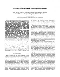
elements with the UT10 Hybrid Simulator. Figure 2 presents an illustration of typical combinations of actuators for different DOFs. Validation tests have been carried out using multi-axial testing apparatus at the University of Toronto. Typical actuator setups for load application to different DOFs are shown in Figure 1. 3. 1.6.2 National Instrument (NI) Hardware In the UT-SIM framework, NICON allows communication between the integration module and the actuator controller. UTNP is used for communication between the integration module and NICON. For the communication between NICON and actuator controller, analog I/O using National Instruments hardware [2017] is used. The main reason for using analog I/O includes: 1. Most actuator controllers can accept commands from external sources through analog signals, and output measured values through analog signals. This approach requires a D/A and A/D conversion process, but the time lag from the conversion process is negligible. In some studies, the analog signals have been used in real-time hybrid simulations as well. 2. The hardware for generating and reading analog signals is generally inexpensive. Unless real time processing is required, generic voltage input and output modules can be purchased at a relatively low cost. It has been confirmed that analog I/O can be used to command and to get measurements from the controllers of the following vendors: MTS, Shore Western, and Instron. Some controllers include SCRAMNet cards such that an integration module and the actuator controller can directly access the same memory address, which is used as a mean of communication. This approach, however, requires proprietary SCRAMNet cards and controllers, which could be quite costly. Figure 1. 4 shows an NI hardware (CompactRIO), which is wired to the Shore Western Controller. Since the setup is intended to control a 6DOF system, the setup requires 6 channels of input to the controller, 6 channels of displacement output, 6 channels of force output, and additional channels to take measurements of a specimen externally. A similar setup is currently used for all other pseudo-dynamic hybrid simulations at the University of Toronto. 1.6.3 Actuator Controller Actuator controllers run a PID control loop based on displacement or force feedback. In some realtime hybrid simulations, the actuator control loop is modified to minimize the time lag coming from the physical system (actuator-specimen). In pseudo-dynamic hybrid simulations, the lag is not an issue. As long as the actuators can impose the target displacement up to a certain level of accuracy, the controller can be used for hybrid simulations.

8

Figure 1. 4: CompactRIO NI Hardware Wired to the Shore Western Controller

The most common limiting factor is usually the flexibility of the reaction system. Most actuators use their internal LVDT as a displacement feedback signal, which is not the actual deformation of

9

the specimen. The actual deformation of the specimen is influenced by the relative stiffness of the specimen and the reaction system. Thus, in many tests, the actual specimen's deformation needs to be externally measured, and then used as a displacement feedback. This approach is somewhat unsafe if a specimen fails abruptly, or if there is any chance that debris such as spalling concrete hits the LVDT. In many applications, the external feedback is used to construct an additional layer of external control loop, for updating the command in Module #2 to Module #4, shown in Figure 1. 2. 1.6.4 Actuators Most actuators in structural testing applications use hydraulic systems. Depending on the number of DOFs, the equipment may consist of a single actuator or several coupled actuators acting simultaneously. In the Structural Testing Facility at the University of Toronto, several unique pieces of equipment are available, all of which can be fully integrated into hybrid simulations using the UT-SIM framework. Some of the equipment that have been integrated in hybrid simulations include the UT10 Hybrid Simulator and the Shell Element Tester [Mojiri et al. 2015a; 2015b], the Column Testing Frame [Giotis et al.], the 6DOF Testing Machine [Sadeghian et al.], and the Uniaxial Shaking Table. For additional information on these testing equipment visit http://www.UT-SIM.ca/hybrid-simulation.html. 1.7

UT-SIM MULTI-PLATFORM NUMERICAL-NUMERICAL HYBRID SIMULATION ELEMENTS

In addition to an integration module, discussed in Section 1.5.2, and a substructure modules, discussed in Section 1.5.3, in a purely numerical hybrid simulation, or in multi-platform hybrid simulations, where at least one of the substructure elements is represented with an analytical model, a communication system must be established to link the structural analysis programs in which the substructure elements are modeled. 1.7.1 Network Interface for Console Applications (NICA) In order to couple structural analysis programs as substructure modules, it is necessary to implement functionalities to communicate with an integration module, to impose target displacements, and to return restoring forces of controlled DOFs back to the integration module. Many structural analysis tools, however, do not have such functionalities. Typically, either the source code of the software needs to be modified, or an interface program needs to be used to allow the software to communicate through the network. These are often referred to as adapter elements as well. Network Interface for Console Applications (NICA) has been developed at the University of Toronto for this purpose [Huang and Kwon; UT-SIM, 2017]. NICA provides exchange of data between an integration module and a numerical substructure module such as OpenSees, ABAQUS or others. Structural analysis programs that can be used as a substructure module through NICA 10

include: (1) Zeus-NL. (2) ABAQUS, (3) OpenSees, and (4) Generic Console Application for other developed finite element programs. 1.8

UT-SIM FRAMEWORK MULTI-PLATFORM HYBRID SIMULATION ELEMENTS

Multi-platform hybrid simulation refers to hybrid simulations in which both analytical and physical substructures could be present. The components of such a simulation includes all those discussed in Sections 1.6 and 1.7. 1.9

REPORT OUTLINE

Complex structures that require advanced analyses could benefit greatly from different advantages that alternative structural analysis programs, or even the testing of physical specimens offer. In such structures, the UT-SIM framework can be used to incorporate several structural analysis programs in the integrated hybrid simulation, leading to accurate, yet efficient analyses. Some examples where coupling structural analysis programs could greatly benefit the structural performance assessment include the following: 1. In the analysis and design of nuclear power plants, it is paramount to account for soilstructure interaction. In such a case, the super-structure (power plant) can be modeled with VecTor 4, and the soil medium can be modeled in OpenSees platform. The two substructures can be integrated into one hybrid simulation using the UT – SIM Framework. 2. In modeling steel structures using OpenSees or S-Frame, usually the connection behavior is modeled with localized calibrated springs. While this is a reasonable approach, the analysis can benefit greatly from modeling the connection in a robust finite element software such as ABAQUS, and coupling the connection substructure with the OpenSees integration module. 3. Many structural analysis programs such as OpenSees do not provide reliable models for predicting the behavior of RC members in shear. Further, the interaction of shear with axial force and bending moment is not considered. Such mechanisms could significantly affect the results and, at times, result in a completely different failure mode for the structure. In such cases, VecTor2 can be used to model the shear critical RC substructure. The substructure can then be coupled with the OpenSees integration module. 4. The seismic performance of a building structure with base isolators is critically affected by the behavior of the base isolation system. In such a case, the base isolators can be physically built and tested in the laboratory, and numerically integrated with the rest of the structure modeled in OpenSees. Such an approach will result in a much more precise seismic performance assessment of the system.

11

Hence, improved multi-platform numerical models, using the distinct advantages of different finite element packages, can greatly enhance the reliability of structural performance assessments. This will ultimately result in improved resilience of the international infrastructure. The main purpose of this report is to provide an outline to assist researchers and structural engineering practitioners in using the UT-SIM framework for the performance assessment of structures. Various hybrid simulations are presented in the following Chapters. In the presented hybrid simulations, different programs are used as integration modules, and as substructure modules. The report and the presented examples will be available for download at http://www.ut-sim.ca/. Each Chapter contains a hybrid simulation example, an overview of the communication system, and a step-by-step procedure to carry out a similar hybrid simulation. In the second Chapter, the example structures that are used in the multi-platform simulations are introduced and presented. In the third Chapter, the procedure for linking two OpenSees models is presented through an example. Chapter 4 presents a numerical multi-platform simulation on the same structure in which OpenSees acts as the integration module, while the substructure is represented with a MATLAB script. Chapter 5 presents a similar example to that presented in Chapter 4, with the substructure presented with a C++ script. In Chapter 6, the procedure to carry out numerical multi-platform simulations using an ABAQUS model as the integration module, and an ABAQUS model as the substructure module is presented. Chapter 7 presents the same procedure as that described in Chapter 6, with the integration module presented with an OpenSees model. Chapter 8 presents the same procedure as that described in Chapter 6, with the substructure module presented with an OpenSees model. Chapter 9 provides an example of the implementation of numerical-experimental hybrid simulations, in which an OpenSees model acts as the integration module and the substructure is represented by a physical spring. Chapter 10 provides an example outlining the procedure for conducting analytical hybrid simulations in which an OpenSees model acts as the integration module, and a VecTor2 model acts as the substructure module. Chapter 11 focuses on the use of high performance computers (HPC) in hybrid simulations within the UT-SIM framework. The procedure is outlined to perform numerical multi-platform simulations in which the integration module is presented by an OpenSeesSP [McKenna and Fenves, 2007] model, running on a HPC, and the substructure module is represented by an OpenSees model, running on a regular operating system. 12

In Chapter 12, the same example as that described for Chapter 10 is presented, with the difference that the integration module is represented by an S-FRAME model. The procedure for using SFRAME as the integration module is outline. It must be noted that the selected examples presented in this report can be extended to any combination of the integration modules and substructure modules, available within the UT-SIM framework, in a completely analogous manner. For instance, In Chapters 3, 6, 7, and 8, the same numerical integration modules and substructure modules are used in different combinations.

13

CHAPTER 2. EXAMPLE STRUCTURES 2.1

INTRODUCTION

This report presents the application of the UT-SIM framework [Huang and Kwon; UT-SIM, 2017] to structural analysis and performance assessment of infrastructures, through simple examples. The example structures, which are used in Chapters 3 to 12, are presented and discussed in this Chapter. 2.2

EXAMPLE STRUCTURE I

2.2.1 General Background and Design Example Structure I is a 2 dimensional one-story one-bay steel frame, on the perimeter of a onestory steel building with large footprint, and is laterally supported with a single concentric buckling-restrained brace (BRB). The structure is located in Vancouver, Canada and is on site class ‘C’.

Figure 2. 1: Illustration of Example Structure I

14

The height of the braced frame is 3.3 meters and the span is 6.0 meters long. The columns are simply supported at their base and the beam is connected to the columns using simple connections without flexural rigidity. Both columns are 254x254x8.0 HSS members of Class C 350W structural steel. The beam element can be assumed to be a rigid element. The core of the BRB consists of a 160mm x 6.4mm steel plate of 300W structural steel. The whole system is supported by a raft foundation on dense soil where the soil settlements are negligible. The seismic weight of the system is 2000 KN (equivalent to a seismic mass of 204 tons) and is lumped at the first story. Figure 2. 1 illustrates a sketch of the structural system. The first mode period is calculated to be 0.597 seconds. 2.2.2 Analytical Substructures Figure 2. 2 illustrates the decomposition of Example Structure I into the integration module and the substructural module. In the sub-structuring scheme, the steel frame without the BRB, shown in Figure 2. 2 (b) acts the integration module, while the BRB element, shown in Figure 2. 2 (c), acts as the substructure module. The sub-structuring decomposition is the same in all hybrid simulations in which Example Structure I is used.

(a)

(b)

(c)

Figure 2. 2: Illustration of the Analytical Models – (a) Standalone Structure, (b) Integration Module, and (c) Substructure Module

2.2.3 Earthquake Ground Record In the examples provided in Chapters 3, 4, 5, and 11, Example Structure I is subjected to an earthquake ground motion record. The system is subjected to the simulated record M6C1 with a scale factor of 0.78 to match the uniform hazard spectrum of Vancouver [Atkinson, 2009]. Figure 2. 3 provides a comparison between the pseudo acceleration response spectrum (PSA) of the scaled record and the Vancouver uniform hazard spectrum (UHS). The shaded area shows the period range of interest as per the provisions of ASCE 7-10 [2010].

15

Figure 2. 3: Pseudo Acceleration Response Spectrum of the Scaled Record vs. the Target Uniform Hazard Spectrum

2.2.4 Pushover Loading In the examples provided in Chapters 6, 7, and 8, a pushover analysis is carried out on Example Structure I. Additional information such as material behavior, modeling assumptions, etc., are discussed in each specific Chapter. 2.3

EXAMPLE STRUCTURE II

2.3.1 General Background and Design Example Structure II is a 2 dimensional two-story one-bay concrete moment resisting frame, located in Vancouver, Canada, on site class ‘C’. The system is supported by a raft foundation rested on dense soil where the soil settlements are negligible. Figure 2. 4 illustrates a sketch of the structure. The structure is designed the using spectral acceleration ordinates specified for Vancouver, and using an RdRo of 3.5. The design is carried out as per the provisions of NBCC 2010 [2010], and CSA A23.3 [2004], without enforcing the seismic provisions. This is carried out to resemble the behaviour of a reinforced concrete moment resisting frame designed prior to the implementation of seismic design guidelines in design standards. The seismic mass in each floor is 30 tons, equivalent to a seismic weight of 294.3 kN. The height of each floor is 3.3 meters, and the span of the frame is 5.0 meters long. The concrete compressive strength, after 28 days, is expected to be f’c = 30 MPa. The yield strength of all reinforcing bars is assumed to be fy = 400 MPa.

16

Figure 2. 4: Illustration of Example Structure II

A diaphragm constraint is assigned to the joints in each floor. A lumped-mass model is used for modeling the seismic mass of the structure at each floor. A modal response spectrum analysis is carried out on the structure, and the periods of the first and the second mode of vibration are determined as 0.436 seconds and 0.126 seconds, respectively, from a preliminary ETABS model. Figure 2. 5 shows the two modes of vibration, as obtained from the preliminary analytical model.

(a)

(b)

Figure 2. 5: Modes of Vibration – (a) First Mode (T1 = 0.436 s), and (b) Second Mode (T 2 = 0.126 s)

17

Using an equivalent static force procedure (ESFP) as per NBCC 2010 [2010] specifications, the base shear is calculated as 99 kN. The base shear calculated using a modal response spectrum analysis method is 102 kN, and is more than 80% of the base shear obtained from the ESFP, and hence does not require additional scaling. The members are designed under gravity loads as well as seismically induced bending moments and shear forces, obtained from the modal response spectrum analysis. Figure 2. 6 shows the typical section for the columns, as well as the floor beam.

(a)

(b)

Figure 2. 6: Frame Member in Example Structure II– (a) Typical Detail for Columns, and (b) Typical Beam Detail

First floor inter-story drift is calculated as 0.525%, and the second floor inter-story drift is calculated as 0.595%. Both inter-story drifts are well below the 2.5% limit for normal importance structures, as specified by NBCC 2010 [2010]. 2.3.2 Analytical Substructures Figure 2. 7 illustrates the decomposition of the Example Structure II into the integration module and the substructural module. The substructure module includes the concrete beam-column joint sub-assemblies on the first floor, shown in Figure 2. 7 (c). The rest of the structure acts as the integration module, as shown in Figure 2. 7 (b). The sub-structuring decomposition is the same in all hybrid simulations in which Example Structure II is used.

=

+

(a)

(b)

(c)

Figure 2. 7: Decomposition of Example Structure II into Analytical Substructures – (a) Standalone Model, (b) Integration Module, (c) Substructural Module

18

2.3.3 Earthquake Ground Record In the example provided in Chapter 10, the example structure is subjected to an earthquake ground motion record. The system is subjected to the simulated record M6C1 with a scale factor of 0.78 to match the uniform hazard spectrum of Vancouver [Atkinson, 2009]. Figure 2. 8 provides a comparison between the pseudo acceleration response spectrum (PSA) of the scaled record and the Vancouver uniform hazard spectrum (UHS). The shaded area shows the period range of interest as per the provisions of ASCE 7-10 [2010]. 2.3.4 Pushover Loading In the example provided in Chapter 12, a pushover analysis is carried out on the structure. Additional information such as material behavior, modeling assumptions, etc., are discussed in each specific Chapter.

Figure 2. 8: Pseudo Acceleration Response Spectrum of the Scaled Record vs. the Target Uniform Hazard Spectrum

2.4

EXAMPLE STRUCTURE III

2.4.1 General Background Example Structure III is a simple two degree of freedom (DOF) mass-spring system shown in Figure 2. 9. The system only experiences motion in the horizontal direction. The masses are free to slide horizontally. Both M1 and M2 are 20.0 kg, while K1 and K2 are 5.0 N/mm. A damping ratio of 2% is assumed for the first and the second mode of the structure. The periods of the structure are calculated as 0.643 seconds and 0.246 seconds for the first and the second modes, respectively.

19

Figure 2. 9: Illustration of Example Structure III

2.4.2 Analytical Substructures Figure 2. 10 illustrates the decomposition of the structure into the analytical substructures. In the experimental hybrid simulation presented in Chapter 11, the first spring (K1) is represented by a physical substructure, as shown in Figure 2. 10 (c), while the rest of the structure acts as the integration module, as shown in Figure 2. 10 (b).

(a)

= (b)

+

(c) Figure 2. 10: Decomposition of the Example Structure III into Analytical Substructures – (a) Standalone Model, (b) Integration module, and (c) Substructure module

20

2.4.3 Earthquake Record In order to limit the time of the experimental hybrid simulation, Arias intensity time bracketing scheme is used to obtain a portion of the M6C1 earthquake ground motion record [Atkinson, 2009] during which 15% to 85% of the seismic input energy is accumulated. The main criteria for choosing such duration is to limit the ground motion length. The resulting ground motion, which is included in the example files as M6C1_1.txt, is 2.4 seconds long. A scaling factor of 3.0 is used for the ground motion. This factor is determined such that the displacement of the physical substructure does not exceed the actuator stroke. Further information on Example Structure III are discussed in Chapter 9.

21

CHAPTER 3. ANALYTICAL HYBRID SIMULATION OPENSEES – OPENSEES 3.1

INTRODUCTION

In this Chapter the step by step procedure for conducting analytical hybrid simulation by coupling two OpenSees [McKenna et al., 2000] models, one acting as the integration module and one as the substructure module, is presented through an example. 3.2

COMMUNICATION OVERVIEW

Shown in Figure 3. 1, is a schematic illustration on how communication is established in numerical multi-platform hybrid simulations in which an OpenSees model acts as the integration module, and one or more OpenSees models act as numerical substructures.

Figure 3. 1: Illustration of Communication and Data Exchange Architecture in Numerical Multi-Platform Hybrid Simulation with an OpenSees Integration Module and OpenSees Substructure Modules

In order to use OpenSees as the main integration module, an OpenSees element termed as SubStructure element has been defined and implemented in OpenSees platform [Huang and Kwon; UT-SIM, 2017]. The SubStructure element is defined to exchange data between the integration module and the substructure module. The properties of the SubStructure element, and the interface nodes as defined in the integration module, are read from the .txt files ‘Kinit.txt’ and ‘Structfile.txt’

22

files, respectively. The ‘Kinit.txt’ and ‘Structfile.txt’ files can be specified/edited by the user, in the same folder where the OpenSees model representing the integration module is located. Further, the interface program NICA, which was defined in Chapter 1, has been developed to externally control the OpenSees substructure analytical model, during the analysis. The interface nodes, as defined in the numerical substructure model, are specified in the ‘NICA.cfg’ file by the user. The ‘NICA.cfg’ file can be edited with any text editor and must be stored in the same folder where the numerical substructure model is located. Communication between the SubStructure element, defined in OpenSees, and the interface program NICA, is enabled by UTNP, which is complied within a Dynamic Link Library, DataExchange.dll. 3.3

EXAMPLE STRUCTURE

The example structure used in this Chapter is Example Structure I, described in Section 2.2. The sub-structuring scheme is the same as that described in Chapter 2, Section 2.2.2. The structure is subjected to the earthquake ground motion, described in Section 2.2.3. 3.4

ANALYTICAL MODELS

In the example numerical hybrid simulation presented herein, first the structural system is modeled in OpenSees platform as a whole. This is carried out to provide a basis for comparing the results of the numerical analysis to the results obtained from the analytical hybrid simulation. Figure 3. 2 (a) shows the complete structure as modeled in OpenSees. Next, the structure is decomposed into two numerical models to act as numerical substructures. In the first numerical substructure, the frame without the BRB specimen is modeled in OpenSees platform. This model will act as the integration module. Figure 3. 2 (b) illustrates the integration module. Afterwards, the BRB specimen is modeled as another numerical substructure in OpenSees platform. This model will act as the substructure module, as shown in Figure 3. 2 (c). When defining the numerical substructures, the sequence of the interface nodes must be consistent, and in the ascending order. The unit systems used in the analytical substructures must also be consistent. In the multi-platform numerical simulation, it is important that an Alpha OS integrator [Combescure and Pegon, 1997] is used for the analysis, and force recorders are not enabled in the OpenSees model. The analysis force outputs can be obtained from the generated .txt files, as discussed in Section 3.6. Displacement recorders can be enabled in the hybrid model.

23

(a)

(b)

(c)

Figure 3. 2: Illustration of the Analytical Models – (a) Standalone OpenSees Model, (b) OpenSees Integration Module, and (c) OpenSees Substructure Module

3.5

PROCEDURE FOR PERFORMING THE NUMERICAL MULTI-PLATFORM SIMULATION

3.5.1 Software Requirements Prior to starting the analytical hybrid simulation steps, it is vital to ensure the following: 1. Extract the content of the ZIP file ‘HSF.zip’, in the example files, and place a copy of the ‘HSF’ folder on the computer drive on which the operating system is installed. This will allow for NICA to run on the system. 2. Ensure that the OpenSees version that is used for the analysis is 2.4.3 (rev 5645). The reason for this step is that the SubStructure OpenSees element has been developed for OpenSees 2.4.3 and has not been updated yet. 3. It is imperative that the two .dll files ‘SubStructure.dll’ and ‘DataExchange.dll’ are placed in the folder from where the OpenSees executable file is running, as shown in Figure 3. 3. If OpenSees is running from the same folder as the model, then the two above-mentioned files must be placed in that folder. The files can be found in the folder containing the example files.

Figure 3. 3: Example Illustration of the Folder Containing the OpenSees Executable File

3.5.2 OpenSees Modeling As previously discussed, the complete structure, the integration module, and the substructure module have been modeled in OpenSees platform. The seismic mass of the system is lumped at the two nodes at the top story. Since the response of the structure in the Y direction is not of 24

interest, only a small mass is assigned to the nodes in the Y direction to avoid numerical instabilities. The HSS columns are modeled using elasticBeamColumn elements to respond in the elastic range. The beam member is defined with a CorotationalTruss element, with its forcedeformation defined using an Elastic uniaxialMaterial. The BRB element is modeled as a CorotationalTruss element, with its force-deformation defined using the Steel02 uniaxialMaterial. A mass proportional damping of 5% is assumed for the first mode. The system is subjected to the simulated record M6C1 with a scale factor of 0.78 to match the uniform hazard spectrum of Vancouver [Atkinson, 2009], as described in Section 2.2.3. Direct time-step integrations of the equations of motion are carried out using a time-step of 0.001s. The first mode period is calculated to be 0.597 seconds. It must be noted, that the substructure module implemented in OpenSees, automatically considers Rayleigh damping. In OpenSees platform, ZeroLength, Truss and CorotationalTruss elements do not automatically take Rayleigh damping into account. Therefore, for consistent results, the – doRayleigh 1 must be added in the script to consider damping both in the complete model as well as the hybrid model. In the present example, since a mass proportional damping is considered this is not necessary. The OpenSees scripts for all three models are provided with the example files. In order to link the two substructures, the OpenSees SubStructure module developed for communication with NICA must be defined in the OpenSees script acting as the numerical integration module. This can be done by the following command: element SubStructure $eleTag –file Structfile.txt –Kinit Kinit.txt; where $eleTag is the unique element tag for the structural component treated as the substructure module. In the current example, the substructure is the BRB element, which has the element tag of 1 in the standalone OpenSees model. The same tag is used in the OpenSees integration module. ‘Structfile.txt’ and ‘Kinit.txt’ are the .txt files in which the information about the location, boundary conditions, and the initial stiffness of substructure module are specified. These .txt files must be created in the same folder in which the numerical model acting as the integration module is located. Specification of the structural properties and the interface nodes for the structure are described in the proceeding sections. 3.5.3 Procedure for linking the two Substructures After creating both OpenSees models, linking the two substructures can be done with the following procedure: 1. If OpenSees is running from the folder in which the OpenSees integration module is located, ensure that the previously mentioned .dll files, ‘SubStructure.dll’ and ‘DataExchange.dll’ are placed in the same folder.

25

2. In the folder where the OpenSees integration module is located, create a .txt file titled ‘Kinit.txt’, which contains the initial stiffness of the substructural element, in the global coordinates. The integration module reads the initial stiffness of the substructural element from this .txt file for starting the analysis, solving the eigenvalue problem, and reporting the periods of the structure. In addition, the displacement commands that are imposed on the substructure module are determined according to the specified stiffness in the ‘Kinit.txt’ file. In the example structure, the substructure module is a truss element. Thus, the stiffness matrices of the element in local and global coordinates take the following form:

KL 

EA  1  1 L  1  1

 cos2    cos sin 0 EA  KG   L   cos2   cos sin  0 

[3.1] cos sin sin 2 

0  cos2  0  cos sin

 cos sin  sin 2 

0  cos sin  sin 2 

0 0 0

0 cos2  cos sin

0 cos sin sin 2 

0

0

0

0

0  0 0  0 0  0

[3.2]

where KL is the element stiffness matrix in the element local coordinates, E is the material modulus of elasticity, A is the element cross sectional area, L is the length of the element, KG is the element stiffness matrix in the global coordinates, and ϴ is the element’s angle with the horizontal axis. In the example problem, we have:

E  200000 MPa

(Modulus Elasticity of Steel Material)

A  160mm  6.4mm  1024mm 2

(Cross Sectional Area of the BRB Steel Core)

L  60002  33002  6847.63mm

(BRB Length)

 3300     Tan 1    28.8  6000 

(BRB Angle with the Horizontal Axis)

By inputting the values into Equation 3.2:

26

12.629  22.962  12.629 6.946   0 0 KG    22.962  12.629   12.629  6.946  0 0 

0  22.962  12.629 0 0  12.629  6.946 0 0 0 0 0 kN  0 22.962 12.629 0 mm 0 12.629 6.946 0  0 0 0 0

Hence, the ‘Kinit.txt’ file for the example structure will be similar to that shown in Figure 3. 4.

Figure 3. 4: ‘Kinit.txt’ File for the Example Structure

3. In the same folder where the integration module is located, a .txt file ‘Structfile.txt’ must be created. The interface nodes and their DOFs, in the integration module, will be specified in this file. Figure 3. 5 shows the node-numbering scheme that is used in the OpenSees integration module, as well as the OpenSees substructure module. Note that the sequence of the interface nodes when defining the integration module and the substructure module must be the same. Figure 3. 6 shows the ‘Structfile.txt’ file for the example structure. As can be observed in Figure 3. 5, the BRB element in the example structure, which is modeled as the substructure module, is connected to nodes 1 and 4. Therefore, ‘NumNode’ is set equal to 2 in the ‘Structfile.txt’, identifying that the substructure module is connected to the integration module through 2 nodes, specified as nodes 1 and 4. Further, it is indicated that each node has three DOFs by setting ‘NumDOFs’ equal to 3.

(a)

(b)

(c)

Figure 3. 5: Node Numbering Scheme in the Numerical OpenSees Models – (a) OpenSees Standalone Numerical Model, (b) OpenSees Integration Module, and (c) OpenSees Substructure Module

27

Figure 3. 6: ‘StructFile.txt’ File Inputs for the Example Structure

4. In the same folder where the integration module is located, create a sub-folder named ‘NICA’ and place all the files accompanying the NICA executable file in this folder. The NICA executable file can be found in the example files. 5. Place the numerical OpenSees model, representing the substructure module, the BRB OpenSees substructure model in the current example, along with any OpenSees source files that are required for the analysis, in the ‘NICA’ folder. 6. Open the ‘NICA.cfg’ file with a text editor and input data according to the example. Figure 3.7 shows the ‘NICA.cfg’ inputs for the example problem. It is important that the Port Number in Figure 3. 7 matches the one specified in Figure 3. 6. The ‘MDL_Type’ number specifies the finite element program in which the substructure module is modeled. Values 1, 2, 3, 4, and 9 can be used for Zeus-NL, OpenSees, ABAQUS [2013], VecTor [Vecchio, 2017], and generic console-in console-out, respectively. In the current example, ‘MDL_Type’ is set equal to 2 to identify that the substructure module is represented by an OpenSees numerical model. ‘MDL_Node’ specifies the control nodes, which are specified in the substructure module. As shown in Figure 3. 5, in the current example these node numbers are consistent with their corresponding nodes numbers in the integration module. Hence, [1 4] is specified. It is essential that the sequence of interface nodes, specified here, is consistent with the nodes specified in Figure 3. 6.

28

Figure 3. 7: ‘NICA.cfg’ File Inputs for the Example Structure

The model dimension must be specified for ‘MDL_Dim’ input. As the example problem is a 2Dimensional problem, the value of 2 is specified for ‘MDL_Dim’. ‘EFF_DOF’ identifies the degrees of freedom for each specified node in ‘MDL_Node’, in the order of X, Y, Z, MX, MY, and MZ. For each DOF, 1 indicates the possibility of movement, where 0 shows the opposite. As the example problem is a 2D structure, modeled in the XY plane, only X, Y, and MZ DOFs are present for each node. Hence, ‘EFF_DOF’ takes the form: 1 1 0 0 0 1. Lastly, in the ‘NICA.cfg’ file, the name of the substructure numerical model must be specified, including the extension. 3.5.4 Hybrid Simulation Execution Upon completion of the above steps, the analytical hybrid simulation can be performed by following the steps outlined below: Open the ‘NICA.exe’ file located in the previously created ‘NICA’ folder. In NICA command window, the message ‘waiting for connection’ will appear. While keeping NICA command window open, run the numerical OpenSees model that acts as the integration module. At this stage, the two models are linked.

29

At this point, the ‘Press Enter to continue’ message will appear in NICA command window. While keeping the integration module OpenSees command prompt open, click on the NICA command prompt and press Enter. The analysis will start. 3.6

DATA POST-PROCESSING

At the conclusion of the analysis, the response of the substructure module, in terms of force and displacement, will be stored in the files ‘Comm_log.log’, and ‘NICA_Data.log’. The former can be found in the directory where the OpenSees integration module runs from. The latter can be found in the NICA subfolder. 3.7

RESULTS COMPARISON

For the example structure, two analyses are carried out. First, the structure as a whole is modeled in OpenSees platform (Complete Model). Next, the structure is decomposed into the integration module (Frame) and the substructure module (BRB element) for performing the analytical hybrid simulation as described above. 3.7.1 Linear Elastic Hybrid Simulation Figure 3. 8 shows the top story lateral displacement time histories, obtained from the complete model and from the numerical multi-platform hybrid simulation, in which the structure is designed to respond in the linear elastic range. Figure 3. 9 shows the structure hysteretic response when subjected to the M6C1 record [Atkinson, 2009], once obtained from the complete model and once from the analytical hybrid simulation. As expected, and as can be observed from Figure 3. 8 and Figure 3. 9, the results obtained from the complete model and the analytical hybrid simulation are identical. 3.7.2 Nonlinear Hybrid Simulation Figure 3. 10 shows the top story lateral displacement time-history, obtained from the complete model and from the analytical hybrid simulation, in which the structure is designed to respond in the inelastic range. Figure 3. 11 shows the structure hysteretic response when subjected to the M6C1 record [Atkinson, 2009], obtained from both the complete model and from the analytical hybrid simulation. As was the case for the linear elastic analysis, and as can be observed from Figure 3. 10 and Figure 3. 11, the results obtained from the complete model and the analytical hybrid simulation are identical.

30

Figure 3. 8: Story Lateral Displacement TH from the Complete Model (Red), and the Hybrid Model (Blue)

Figure 3. 9: Structure Hysteretic Response from the Complete Model (Red), and the Hybrid Model (Black)

31


Figure 3. 11: Hysteretic Response Curves from the Complete Model (Red), and the Hybrid Model (Blue)

32

CHAPTER 4. ANALYTICAL HYBRID SIMULATION OPENSEES – MATLAB 4.1

INTRODUCTION

In many applications, researchers may be interested in developing finite element models using generic programming languages. The UT-SIM framework has the feature that numerical models that have been developed by programming languages such as MATLAB, C++, etc. can be integrated into the numerical model as substructure modules. This feature of the UT-SIM framework is developed to overcome any potential limitations that may be present in available finite element packages. In this Chapter the step by step procedure for conducting numerical hybrid simulation by coupling an OpenSees [McKenna et al., 2000] model, as the integration module, with a MATLAB script, representing the substructure module, is presented. 4.2


Shown in Figure 4. 1, is a schematic illustration on how communication is established in numerical multi-platform hybrid simulations in which an OpenSees model acts as the integration module, and the substructural module is represented by a MATLAB script.

Figure 4. 1: Illustration of Communication and Data Exchange Architecture in Numerical Multi-Platform Hybrid Simulation with an OpenSees Integration Module and MATLAB Substructure Modules

33

Similar to the previous Chapter, in order to use OpenSees as the main integration module, the same OpenSees element termed the SubStructure element is used along with the ‘Kinit.txt’ and ‘Structufile.txt’ .txt files. Contrary to Chapter 3, there is no need to use NICA for externally controlling the substructure numerical model, in MATLAB. The substructure, represented by a MATLAB script, can directly react to commands from the integration module. The reason is that a script similar to NICA’s is implemented in the MATLAB substructure. Communication between the SubStructure element, defined in OpenSees, and the MATLAB substructure, is enabled by UTNP, which is complied within a Dynamic Link Library, DataExchange.dll. 4.3

EXAMPLE STRUCTURE

Example Structure I, described in Chapter 2 is used for the simulation. The general background and the decomposition of the system into analytical sub-structures is identical to that presented in Chapter 3. The only difference in this section is that the response of the BRB specimen is obtained from a MATLAB script, as the substructure module, rather than the use of an OpenSees substructure in conjunction with NICA. Figure 4. 2 shows the decomposition of the structure into the numerical substructures.

(a)

(b)

(c)

Figure 4. 2: Illustration of the Analytical Models – (a) Standalone OpenSees Model, (b) OpenSees Integration Module, and (c) Substructure Module Represented in MATLAB

It must be noted that NICA is a C++ based interface program. As it is possible to have a script similar to NICA’s in MATLAB, the use of NICA in this example will not be necessary. The required MATLAB script for performing the hybrid simulation is provided in the example files. 4.4

PROCEDURE FOR PERFORMING ANALYTICAL HYBRID SIMULATION

4.4.1 General Recommendations Prior to starting the numerical hybrid simulation steps, it is recommended to do the following: 1. Create a folder entitled ‘MATLAB_Substructure’. This is the folder where the MATLAB script and the necessary files can be saved. 34

2. Create a folder entitled ‘OpenSees_Integration’. In this folder, the integration module and the necessary files will be saved. 3. It is further recommended to have the complete model located in a directory close to these folders. The Complete model can provide a basis for comparing the results of the numerical analysis with the results obtained from the analytical hybrid simulation. 4.4.2 Software Requirements Prior to staring the numerical hybrid simulation steps, it is vital to ensure the following: 1. Extract the content of the ZIP file ‘HSF.zip’ and place a copy of the ‘HSF’ folder on the computer drive on which the operating system is installed. 2. Ensure that the OpenSees version that is used for the analysis is 2.4.3 (rev 5645). The reason for this step is that the SubStructure OpenSees element was developed for OpenSees 2.4.3 and has not been updated yet. 3. It is imperative that the two .dll files ‘SubStructure.dll’ and ‘DataExchange.dll’ are placed in the folder from where the OpenSees executable file is running, as shown in Figure 4. 3. If OpenSees is running from the same folder as the model that represents the n module, then the two above-mentioned files must be placed in that folder. The files can be found in the folder containing the example files. 4. It is further necessary that the files ‘DataExchange.dll’ and ‘DataExchange.h’ are placed in the folder from which the MATLAB script, representing the substructure module, is running. Following the recommended steps outlined in section 4.4.1, the ‘MATLAB_Substructure’ folder would take the form shown in Figure 4. 4. The MATLAB script ‘Server.m’ is a MATLAB file containing the script for linking the substructure to the integration module, as well as the numerical model of the substructure module.

Figure 4. 3: Example Location of OpenSees Executable file and the .dll Files

35

Figure 4. 4: Location of the MATLAB Script, Representing the Substructure Module and the Communication System with Necessary Files

4.4.3 OpenSees Modeling (Integration Module) The Complete OpenSees model, used for validating the results of the hybrid simulation, is identical to that discussed in Chapter 3. The same holds for the OpenSees script developed as the integration module. In addition, all the analysis assumptions are identical to those considered in Chapter 3. The OpenSees scripts for the complete model and the integration module are provided in the example files. The analysis assumptions (ground motion, structural properties, etc.), are the same as those in Chapter 3. The only deviations are: (1) The communication of the integration module and the substructure module is carried out by the MATLAB script ‘Server.m’ instead of NICA, and, (2) The structural properties of the substructure module is modeled in the MATLAB script ‘Server.m’. Similar to Chapter 3, in order to link the two substructures, the SubStructure element developed for OpenSees platform [Huang and Kwon; UT-SIM, 2017], must be defined in the integration module, to represent the substructural element. This can be done by the following command: element SubStructure $eleTag –file Structfile.txt –Kinit Kinit.txt; where $eleTag is the unique element tag for the structural component treated as the substructure module. In the current example, the substructure module is the BRB specimen, which has the element tag of 1 in the complete model. For the hybrid simulation, the same tag is used in the OpenSees model that act as the integration module. ‘Structfile.txt’ and ‘Kinit.txt’ are the .txt files in which the information about the location, boundary conditions, and the initial stiffness of the substructure element are specified. These .txt files must be created in the same folder in which the OpenSees model, representing the integration module, is located. This is further explained in the proceeding section. 4.4.4 MATLAB Script (Sub-Structure Module) The MATLAB script developed to handle the communication between the integration module and the substructure module, ‘Server.m’, is provided in the example files. It is important that the values of the ‘Kinit’ matrix in the script are updated to values corresponding to the initial global stiffness of the substructure element, in global coordinates. The initial global stiffness of the BRB specimen,

36

in the example structure, is determined in Chapter 3. Hence, the ‘Kinit’ matrix in the MATLAB script takes the following form:

12.629  22.962  12.629 6.946   0 0 KG    22.962  12.629   12.629  6.946  0 0 

0  22.962  12.629 0 0  12.629  6.946 0 0 0 0 0 kN  0 22.962 12.629 0 mm 0 12.629 6.946 0  0 0 0 0

In addition to the stiffness matrix, the port number that is specified in the MATLAB script is of importance. The port number that will be specified for the integration module will match the port number in the MATLAB script. It must be noted that the presented MATLAB script is developed for a linear elastic analysis. However, a similar script can be developed for nonlinear dynamic analyses in a completely analogous manner. 4.4.5 Procedure for linking the two Substructures After creating the OpenSees integration module and the MATLAB script, linking the two substructures can be done using the following procedure: 1. If OpenSees is running from the folder in which the integration module is located, it must be ensured that the previously mentioned .dll files, ‘SubStructure.dll’ and ‘DataExchange.dll’ are placed in the folder. 2. In the folder where the integration module is located, create a .txt file titled ‘Kinit.txt’, which contains the initial stiffness of the substructure module, in the global coordinates. The integration module reads the initial stiffness of the substructure module from this .txt file for starting the analysis, solving the eigenvalue problem and reporting the periods of the structure. In addition, the displacement commands that are imposed on the substructure module are determined according to the specified stiffness in the ‘Kinit.txt’ file. The initial global stiffness of the substructure module, for the current example, is determined in Chapter 3 and presented in Section 4.4.4. Hence, the ‘Kinit.txt’ file for the example structure will be as shown in Figure 4. 5. 3. In the same folder where the integration module is located, a .txt file ‘Structfile.txt’ must be created. The interface nodes and their DOFs, in the integration module, will be specified in this file. Figure 4. 6 shows the ‘Structfile.txt’ file for the example structure.

37

Figure 4. 5: ‘Kinit’ File for the Example Structure

The structure under consideration is a 2-dimensional problem, and hence, Ndm is specified as 2. It must be ensured that the port number that is specified here matches the port number specified in the MATLAB script (refer to the MATLAB script in the example files).

Figure 4. 6: ‘Structfile.txt’ File for the Example Structure

38

In the example structure the BRB element, considered as the substructure module, is connected to nodes 1 and 4 (Figure 3. 5 in Chapter 3). Therefore, ‘NumNode’ is set equal to 2 in the ‘Structfile.txt’, identifying that the slave substructure is connected to the master model through 2 nodes, specified as nodes 1 and 4. Further, it is indicated that each node has three DOFs by setting ‘NumDOFs’ equal to 3. The rest of the inputs are self-explanatory. 4.4.6 Hybrid Simulation Execution Upon completion of the above steps, the analytical hybrid simulation can be performed by following the steps outlined below: Open the ‘Server.m’ MATLAB script which contains the structural properties of the slave substructure and handles the communication between the integration module and the substructure module. Run the MATLAB script. Wait until the program gives the warning ‘loadlibrary(…)’. While keeping the MATLAB script window open, run the OpenSees model that acts as the integration module. At this stage, the two models are linked. No further actions are required and the analysis will start. 4.5


Upon the conclusion of the analysis, the response of the substructure element, in terms of force and displacement, will be stored in the file ‘Comm_log.log’. This file can be found in the folder containing the integration module. 4.6

RESULTS COMPARISON

For the example structure, two analyses are carried out. First, the structure as a whole is modeled in OpenSees platform (Complete Model). Next, the structure is decomposed into the integration module (Frame) and the substructure module (BRB element) for performing the analytical hybrid simulation as described above. In the present Chapter, only a linear hybrid simulation is carried out to outline the procedure. A nonlinear hybrid simulation can be carried out in a completely analogous manner, by adjusting the MATLAB script accordingly. Figure 4. 7 shows the top story lateral displacement time histories, obtained from the complete model and from the analytical hybrid simulation, in which the structure is designed to respond in the linear elastic range. Figure 4. 8 shows the structure hysteretic response when subjected to the M6C1 record [Atkinson, 2009], obtained from both the complete model and from the analytical hybrid simulation. As expected, and as can be observed from Figure 4. 7 and Figure 4. 8, the results obtained from the complete model and the analytical hybrid simulation are identical.

39



40

CHAPTER 5. ANALYTICAL HYBRID SIMULATION OPENSEES – C++ 5.1

INTRODUCTION

As an extension of the previous Chapter, in this Chapter, the step by step procedure for conducting analytical hybrid simulation by coupling an OpenSees [McKenna et al., 2000] model, as the integration module, with a C++ script, representing the substructure module, is presented. 5.2


Shown in Figure 5. 1, is a schematic illustration on how communication is established in numerical multi-platform hybrid simulations in which an OpenSees model acts as the integration module, and the substructural module is represented by a C++ script.

Figure 5. 1: Illustration of Communication and Data Exchange Architecture in Numerical Multi-Platform Hybrid Simulation with an OpenSees Integration Module and C++ Substructure Modules

Similar to previous Chapters, in order to use OpenSees as the main integration module, the same OpenSees element termed as SubStructure element is used along with the ‘Kinit.txt’ and ‘Structufile.txt’ .txt files. Contrary to Chapter 3, there is no need to use NICA for externally controlling the substructure analytical model, in C++. The substructure, represented by the C++ script, can directly react to

41

commands from the integration module. The reason is that a script similar to NICA’s is implemented in the C++ substructure. Communication between the SubStructure element, defined in the OpenSees integration module, and the C++ substructure, is enabled by UTNP, which is complied within a Dynamic Link Library, DataExchange.dll. 5.3

EXAMPLE STRUCTURE

Example Structure I, described in Chapter 2 is used for the simulation. The general background and the decomposition of the system into numerical substructures is identical to that presented in Chapter 3. The only difference in this section is that the response of the BRB specimen is obtained from a C++ script, as the substructure module, rather than the use of an OpenSees substructure in conjunction with NICA. Figure 5. 2 shows the decomposition of the structure into the analytical substructures.

(a)

(b)

(c)

Figure 5. 2: Illustration of the Analytical Models – (a) Standalone OpenSees Model, (b) OpenSees Integration Module, and (c) Substructure Module Represented in C++

It must be noted that NICA is a C++ based interface program. As it is possible to include a script similar to NICA’s in the sub-structure C++ script, the use of NICA in this example will not be necessary. The required C++ script for performing the multi-platform analytical hybrid simulation is provided in the example files. 5.4

PROCEDURE FOR PERFORMING ANALYTICAL HYBRID SIMULATIONS

5.4.1 General Recommendations Prior to starting the analytical hybrid simulation steps, it is recommended to do the following: 1. Create a folder entitled ‘CPP_Substructure’. This is the folder where the C++ script and the necessary files for compiling the code can be saved. 2. Create a folder entitled ‘OpenSees_Integration’. In this folder, the integration module and the necessary files will be saved.

42

3. It is further recommended to have the complete model located in a directory close to these folders. The Complete model can provide a basis for comparing the results of the numerical analysis with the results obtained from the analytical hybrid simulation. 5.4.2 Software Requirements Prior to starting the analytical hybrid simulation steps, it is vital to ensure the following: 1. Extract the content of the ZIP file ‘HSF.zip’ and place a copy of the ‘HSF’ folder on the computer drive on which the operating system is installed. 2. Ensure that the OpenSees version that is used for the analysis is 2.4.3 (rev 5645). The reason for this step is that the SubStructure OpenSees element was developed for OpenSees 2.4.3 and has not been updated yet. 3. It is imperative that the two .dll files ‘SubStructure.dll’ and ‘DataExchange.dll’ are placed in the folder from where the OpenSees executable file is running, as shown in Figure 5. 3. If OpenSees is running from the same folder as the OpenSees integration module, then the two above-mentioned files must be placed in that folder. The files can be found in the folder containing the example files. 4. It is further necessary that the files ‘DataExchange.dll’ and ‘DataExchange.h’ are placed in the folder from which the C++ script, representing the substructure module, is running. Following the recommended steps outlined in section 5.4.1, the ‘CPP_Substructure’ folder would take the form shown in Figure 5. 4. The file ‘Server.cpp’ is a C++ script file containing the code for linking the substructure to the integration module, as well as the properties of the substructure module. The ‘Server’ folder contains the necessary files for compiling the C++ code into an executable file. The ‘Server.exe’ file is the executable file that is created after compiling the C++ code, using visual studio. All these files can be found in the example files. The procedure for compiling the C++ script is explained in the upcoming sections.

Figure 5. 3: Example Location of the OpenSees Executable File and the.dll Files

43

Figure 5. 4: Location of the C++ Script, Representing the Substructure Module and the Communication System with Necessary Files

5.4.3 OpenSees Modeling (Integration Module) The Complete OpenSees model, used for validating the results of the hybrid simulation, is identical to that presented in Chapter 3. The same holds for the OpenSees script developed as the integration module. In addition, all the analysis assumptions are identical to those considered in Chapter 3. The analysis assumptions (ground motion, structural properties, etc.), can be found in Chapter 3. The only deviations are: (1) The communication of the integration module and the substructure module is carried out by the C++ script ‘Server.cpp’, instead of NICA, and (2) The structural properties of the substructure module is modeled in the C++ script ‘Server.cpp’. Similar to Chapter 3, in order to link the two substructures, the SubStructure element developed for OpenSees platform, must be defined in the integration module, to represent the substructure element. This can be done by the following command: element SubStructure $eleTag –file Structfile.txt –Kinit Kinit.txt; where $eleTag is the unique element tag for the structural component treated as the substructure module. In the current example, the substructure module is the BRB specimen, which has the element tag of 1 in the complete model. The same tag is used in the OpenSees model, representing the integration module. ‘Structfile.txt’ and ‘Kinit.txt’ are the .txt files in which the information about the location, boundary conditions, and the initial stiffness of the substructure module are specified. These .txt files must be created in the same folder in which the OpenSees model, representing the integration module, is located. This is further explained in the proceeding section. 5.4.4 C++ Script (Sub-Structure Module) The C++ script developed to handle the communication between the integration module and the substructure module, ‘Server.cpp’, is provided in the example files. It is important that the values of the ‘Kinit’ matrix in the script are updated to values corresponding to the initial global stiffness of the substructure element, in global coordinates. The initial global stiffness of the BRB specimen, in the example structure, is determined in Chapter 3. Hence, the ‘Kinit’ matrix in the C++ script takes the following form:

44

12.629  22.962  12.629 6.946   0 0 KG    22.962  12.629   12.629  6.946  0 0 

0  22.962  12.629 0 0  12.629  6.946 0 0 0 0 0 kN  0 22.962 12.629 0 mm 0 12.629 6.946 0  0 0 0 0

In addition to the stiffness matrix, the port number that is specified in the C++ script is of importance. The port number that will be specified for the integration module will match the port number in the C++ script. It must be noted that the presented C++ script is developed for linear elastic analyses. However, a similar script can be developed for nonlinear dynamic analyses in a completely analogous manner. 5.4.5 Procedure for linking the two Substructures After creating the OpenSees integration module and the C++ script, linking the two substructures can be done using the following procedure: 1. If OpenSees is running from the folder in which the integration module is located, ensure that the previously mentioned .dll files, ‘SubStructure.dll’ and ‘DataExchange.dll’ are placed in the folder. 2. In the folder where the integration module is located, create a .txt file titled ‘Kinit.txt’, which contains the initial stiffness of the substructure module, in the global coordinates. The integration module reads the initial stiffness of the substructure module from this .txt file for starting the analysis, solving the eigenvalue problem and reporting the periods of the structure. In addition, the displacement commands that are imposed on the substructure module are determined according to the specified stiffness in the ‘Kinit.txt’ file. The initial global stiffness of the substructure module, for the current example, is determined in Chapter 3 and presented in Section 5.4.4. Hence, the ‘Kinit.txt’ file for the example structure will be as shown in Figure 5. 5.

Figure 5. 5: ‘Kinit.txt’ File for the Example Structure

45

3. In the same folder where the OpenSees model, representing the integration module, is located a txt file ‘Structfile.txt’ must be created. The interface nodes and their DOFs, as defined in the integration module, will be specified in this file. Figure 5. 6 shows the ‘Structfile.txt’ file for the example structure.

Figure 5. 6: ‘Structfile.txt’ File for the Example Structure

The structure under consideration is a 2-dimensional problem, and hence, Ndm is specified as 2. It must be ensured that the port number that is specified here matches the port number specified in the C++ script (refer to the C++ script in the example files). In the example structure the BRB element, considered as the substructure module, is connected to nodes 1 and 4 (Figure 3.5 in Chapter 3). Therefore, ‘NumNode’ is set equal to 2 in the

46

‘Structfile.txt’, identifying that the substructure module is connected to the integration module through 2 nodes, specified as nodes 1 and 4. Further, it is indicated that each node has three DOFs by setting ‘NumDOFs’ equal to 3. The rest of the inputs are self-explanatory. 5.4.6 Compiling the C++ Script into an Executable File After finalizing the C++ script, the script must be compiled into an executable file in order to run the analysis. This can be done by using Microsoft Visual Studio Professional. The procedure for compiling a C++ script, using Microsoft Visual Studio Professional 2012 is outlined below in windows 8: 1. First, it must be ensured that Kinit and the port number are adjusted accordingly, in the C++ script. 2. It must be noted that the ‘DataExchange.dll’ file is a 64-bit file. Hence, it is of importance that the C++ script is compiled in 64-bit as well. 3. Open the ‘Server.cpp’ file with Visual Studio Professional 2012. 4. Navigate through File > New > Project. 5. Activate Visual C++ template from the Templates tab. 6. Activate Win32 Console Application. 7. Deselect the ‘Create directory for solution’ option. 8. Click on OK. 9. In the ‘Welcome to the Win32 Application Wizard’, click on Next. 10. In the ‘Application Settings’ window, select the ‘Empty project’ option. Click on Finish. 11. In the Solution Explorer, right-click on the ‘created project’ and select ‘properties’. 12. Choose the ‘configuration manager’ and open the configuration manager dialog box. 13. Use the dropdown list for the ‘Active solution platform’, and select ‘new’ to create a new solution platform dialog box. 14. In the ‘Type or select the new platform’, select a 64-bit platform. 15. After clicking on OK, the platform that was created (x64) will appear in the ‘Active solution platform’. 16. Select Close. 17. Select OK. 18. Right-click on the Source Files, and select Add > Existing Item. 19. Browse, locate and select the Server.cpp script.

47

20. Select the ‘Build’ tab and select ‘Build Solution’. 21. The .exe file will be stored in a default location that will be shown at the bottom of the screen. 22. Copy the .exe file to a convenient location, preferably close to the OpenSees integration module. 5.4.7 Hybrid Simulation Execution Upon completion of the above steps, the analytical hybrid simulation can be performed by following the steps outlined below: Run the ‘Server.exe’ executable file that is located in the sub-structure folder. The message ‘waiting for connection’ will appear. Run the OpenSees integration module. No further actions are required and the analysis will start. 5.5


Upon the conclusion of the analysis, the response of the specimen, in terms of force and displacement, will be restored in the file ‘Comm_log.log’. This file can be found in the folder containing the integration module. 5.6

RESULTS COMPARISON

For the example structure, two analyses are carried out. First, the structure as a whole is modeled in OpenSees platform (Complete Model). Next, the structure is decomposed into the integration module (Frame) and the substructure module (BRB element) for performing the analytical hybrid simulation as described above. In this Chapter, only a linear hybrid simulation is carried out to outline the procedure. A nonlinear hybrid simulation can be carried out in a completely analogous manner, by adjusting the C++ script accordingly. Figure 5. 7 shows the top story lateral displacement time histories, obtained from the complete model and from the analytical hybrid simulation, in which the structure is designed to respond in the linear elastic range. Figure 5. 8 shows the structure hysteretic response when subjected to the M6C1 record [Atkinson, 2009], obtained from both the complete model and from the analytical hybrid simulation. As expected, and as can be observed from Figure 5. 7 and Figure 5. 8, the results obtained from the complete model and the analytical hybrid simulation are identical.

48



49

CHAPTER 6. ANALYTICAL HYBRID SIMULATION ABAQUS – ABAQUS 6.1

INTRODUCTION

In this Chapter the step by step procedure for conducting analytical hybrid simulation by coupling an ABAQUS [2013] model, as the integration module, with another ABAQUS model, representing the substructure module, is presented. 6.2


Similar to the SubStructure element defined for OpenSees, in order to use ABAQUS as the integration module, a User Element (UEL) has been developed [Huang and Kwon; UT-SIM, 2017] for ABAQUS. There are two alternative methods for integrating ABAQUS as the substructure module, in a multi-platform hybrid simulation. In one approach, the interface program NICA, discussed in Chapter 1, can be used. The procedure will be similar to that discussed in Chapter 3. A schematic illustration of the communication and data exchange architecture in such a case is presented in Figure 6. 1.

Figure 6. 1: Illustration of Communication Architecture in Numerical Multi-Platform Hybrid Simulation with an ABAQUS Integration Module and ABAQUS Substructure Modules, with Using NICA

In the other approach, a UEL for ABAUQS substructures has been developed to facilitate direct communication between the integration module and the ABAQUS substructure module. Hence, using NICA will not be necessary. A schematic illustration of the communication and data exchange architecture in such a case is presented in Figure 6. 2.

50

Figure 6. 2: Illustration of Communication Architecture in Numerical Multi-Platform Hybrid Simulation with an ABAQUS Integration Module and ABAQUS Substructure Modules, without Using NICA

Communication between the UEL for the integration module and NICA (Figure 6. 1), or UEL for the substructure module (Figure 6. 2), is enabled by UTNP which is complied within a Dynamic Link Library, DataExchange.dll. In the current example, the second communication scheme is adopted. 6.3

EXAMPLE STRUCTURE

Example Structure I, described in Chapter 2 is used for the simulation. The general background and the decomposition of the system into analytical substructures is identical to that presented in Chapter 3. The difference in this section is that the BRB specimen is modeled using a solid element in ABAQUS, as the substructure module. In addition, the integration module is modeled in ABAQUS, using frame elements. Figure 6. 3 shows the decomposition of the structure into the analytical substructures.

(a)

(b)

(c)

Figure 6. 3: Illustration of the Analytical Models – (a) Standalone ABAQUS Model, (b) ABAQUS Integration Module Using Frame Elements, and (c) ABAQUS Substructure Module Using Solid Elements

6.4

ASSUMPTIONS/ANALYSIS

A push over analysis is carried out on the example structure. The pushover analysis is first carried out on a standalone analytical model of the structure as a whole, in ABAQUS, using frame elements. Figure 6. 4 shows a screenshot of the standalone ABAQUS model of the structure with frame elements, in extruded view.

51

Next, the structure is decomposed into two analytical substructures, modeled in ABAQUS, and a push over analysis is carried out on the multi-platform model. The frame substructure is modeled in ABAQUS using frame elements, which acts as the integration module. Figure 6. 5 (a) shows a screenshot of the integration module modeled in ABAQUS using frame elements. The BRB is modeled in ABAQUS, which acts as the substructure module. Solid elements are used for modeling the BRB specimen in ABAQUS. C3D8R 8-node linear brick elements with reduced integration elements are used as the mesh elements. Figure 6. 5 (b) shows the substructural module, as modeled in ABAQUS.

(a)

(b)

Figure 6. 4: Standalone ABAQUS model of the Structure, Using ABAQUS– (a) 3D View, (b) 2D View

+

(a)

(b)

Figure 6. 5: Analytical Substructures – (a) ABAQUS Integration Module Using Frame Elements, and (b) ABAQUS Substructural Module Using Solid Elements

Since the model is created for demonstration purposes, a mesh-sensitivity analysis is not carried out. The element is modeled such that it would yield in both tension and compression, as expected from BRB elements. 52

In all models, a simple bilinear material behavior is assumed for the BRB steel material. The yield strength is assumed as 300 MPa, as expected for 300W steel. The post-yield modulus is assumed to be 1% of the elastic material modulus. The assumed stress-strain response is shown in Figure 6. 6. A linear elastic behavior is assumed for the beam and the columns, as they are not expected to undergo nonlinear deformations.

Figure 6. 6: Stress-Strain Response of the Buckling-Restrained Braced Steel Material

6.5

ACCESSING ABAQUS SUBROUTINE

Hybrid simulation and communication with ABAQUS substructures is carried out through ABAQUS subroutines. Therefore, in order to facilitate hybrid simulations with ABAQUS substructures, access to ABAQUS subroutines must be established. In order to do this, ABAQUS, must be linked with Visual Studio and Intel Composer XE. In this section, the procedure for accessing ABAQUS subroutines, by linking ABAQUS 6.13-1, Microsoft Visual Studio 2012, and Intel Composer XE 2013, is outlined. Note that the version of the programs may not be necessary, but they are recommended as they have been tested. 1. Have ABAQUS 6.13-1 installed on the operating system. 2. Have Microsoft Visual Studio 2012 installed on the operating system. 3. Have Intel Composer XE 2013 installed on the operating system. 4. Locate the files ‘ifort.exe’, and ‘Ifortvars.bat’ on the operating system. Their typical locations are provided below: 

‘ifort.exe’ Location: C:\Program Files (x86)\Intel\Composer XE 2013\bin\intel64



‘Ifortvars.bat’ Location:

C:\Program Files (x86)\Intel\Composer XE 2013\bin

53

5. Have the location of the above-mentioned files saved in .txt files, located close to where all the files and folders for the simulation will be restored. 6. Open the Control Panel window and go to Control Panel > All Control Panel Items > System. Alternatively, right-click on the ‘This PC’ main folder on the system, and select properties. 7. In the System window click on ‘Advanced system settings’ menu. 8. In the ‘Advanced’ tab, click on the ‘Environment Variables’ icon. 9. In the User variables, select Path. It is required to add the locations for ‘ifort.exe’, and ‘Ifortvars.bat’ to the Path. 10. If Path is not in the User Variable items, click on New and add Path as the Variable name. In the Variable Value copy/paste the location of ‘ifort.exe’ and ‘Ifortvars.bat’, separated with a semicolon. If the Path is already present, click on Path, then Edit, and add the location of ‘ifort.exe’, and ‘Ifortvars.bat’, separated with a semicolon to the existing ones. Then click on OK. 11. Go to the Command directory in the ABAQUS folder on the operating system. This is typically located at ‘C:\SIMULIA\Abaqus\Commands’. 12. Open the file ‘abq6131.bat’, using a note pad or any txt editor. 13. After the line ‘@echo off’, add the following line: ‘@call ifortvars.bat intel64 vs2012’. Save and close the file. Figure 6. 7 shows an example of how the ‘abq6131.bat’ file should look like after the edit.

Figure 6. 7: Screenshot of the Edited ‘abq6131.bat’ File

14. At this stage, ABAQUS is linked with Visual Studio and Intel Composer XE 2013. It is recommended to check if the procedure is carried out properly. This can be done by the following steps: A. Open a command window. This can be done by opening the start menu and typing ‘cmd’.

54

B. Type ‘abaqus –verify’ and enter. The command prompt will generate a list of commands that can be used. C. In the current example, the aim is to verify the ‘User Subroutine’. Therefore, use the command ‘abq6131 verify –user_std’. Note that the term ‘abq6131’ could be different in other systems. The specific term for the system is generated in the command prompt after step B. Important Note: It is imperative that the ‘Microsoft Parallel Processing MPI Interface’ version that is installed on the operating system is compatible with the installed ABAQUS. Typically, the ABAQUS installation is accompanied with the compatible version. For instance, in the current example where ABAQUS 6.13 is used, the compatible MPI version is ‘mpi_3.0x64.msi’. Therefore, the existing MPI versions on the system were uninstalled and replaced with the compatible one. A better alternative is to check the MPI version that is installed on the system, prior to installing ABAQUS. If the version is not compatible, uninstall it. This way, the compatible version will be automatically installed with ABAQUS. D. At this stage, the ‘…PASS’ message will be generated in the command prompt, indicating that user subroutine is accessible now, as shown in Figure 6. 8.

Figure 6. 8: PASS Message as Observed in the Command Prompt

6.6

ADJUSTING THE DATA EXCHANGE LIBRARY FOR ABAQUS

In order to perform analytical hybrid simulations, using ABAQUS substructures, it is essential to adjust the data exchange library for ABAQUS. This can be done, using the following steps: 1. The required files for this procedure are included in the example files. The specific files are ‘DataExchange.dll’, ‘DataExchange.h’, and ‘DataExchange.lib’. 55

2. Create a copy of the files ‘DataExchange.dll’, ‘DataExchange.h’, and ‘DataExchange.lib’, in the ABAQUS bin folder on the system. The typical location of this folder is ‘C:\SIMULIA\Abaqus\6.13-1\code\bin’. 3. Locate file ‘abaqus_v6.env’ at ‘C:\SIMULIA\Abaqus\6.13-1\SMA\site’. ‘abaqus_v6.env’ with a notepad or any txt editor.

Open

4. Scroll down to find the ‘link_sl’ variable. In the last line, add the address for the newly created DataExchange.lb file in step 2 as ‘C:\SIMULIA\Abaqus\6.131\code\bin\DataExchange.lib’. Single quotation marks must be used. In addition, it must be noted that for ABAQUS, double backslashes (\\) should be used rather than a single backslash (\). Therefore, the added address would be ‘'C:\\SIMULIA\\Abaqus\\6.131\\code\\bin\\DataExchange.lib'’. The result of this procedure is shown in Figure 6. 9:

Figure 6. 9: The Result of the Procedure Described in Step 4

5. Save and close the txt file. 6. Upon the completion of this procedure, execution of hybrid simulation with ABAQUS as one of the analytical substructures will be possible. 6.7

PROCEDURE FOR PERFORMING HYBRID SIMULATION USING ABAQUS SUBSTRUCTURES

In order to use ABAQUS models as analytical substructures, first the ABAQUS models must be created. This can be done using the ABAQUS visual interface. Afterwards, the procedure provided in Section 6.7.1, and the procedure provided in Section 6.7.2 must be followed for the ABAQUS integration and substructure modules, respectively. Upon the completion of these steps, use of ABAQUS models as numerical integration and substructure modules will be possible. The procedure in the following sections are described with the aid of the provided example in this Chapter. For new analytical hybrid simulations using ABAQUS substructures, the same procedures can be used in a completely analogous manner. Therefore, before following the steps provided below, download the example folder. In the example folder, the subfolder ‘AbaInt’ contains the ABAQUS integration module files, and the subfolder ‘AbaSub’ contains the ABAQUS substructure module files. 6.7.1 Procedure Required for Using ABAQUS Models as Integration Modules 1. Create the ABAQUS model that acts as the integration module, using the ABAQUS visual interface. In the example folder, the subfolder ‘ABQ-Integration’ contains the original 56

ABAQUS model that was created within the ABAQUS visual interface to represent the Integration module. 2. As discussed previously, analytical substructuring using ABAQUS is carried out by using ABAQUS subroutines. The subroutines for ABAQUS substructuring that are used in UTSIM framework are a modified version of the ones developed by Shellenberg et al. [2008; 2009]. Folder ‘AbaInt’ includes the subroutine script for the integration module, used for this example. The file ‘IntSub.for’ is the subroutine script in the current example. Note that in mac operating systems and Linux, the file takes the form ‘ÌntSub.f`’. The same subroutine file can be used for other examples and must be stored in the same folder from which the ABAQUS integration module is running from. 3. Note that the only information that may require editing in the ‘IntSub.for’ file is the IP number (line 355 in integration subroutine). The IP number is only adjusted when a hybrid simulation is carried out using several operating systems. 4. Upon completion of the FE model, save the model to a convenient location close to the example files. 5. After saving the file, create a job. 6. Right-click on the created job and select ‘Write Input’. 7. An input file, ‘job1.inp’ will be generated in the directory where the ABAQUS file is stored. 8. Afterwards, the input file must be modified to match the required format for ABAQUS sub-structuring. A template for the required format is provided in the example files termed ‘Abq Intstructure Template’. Input file ‘AbaInt.inp’, in the ‘AbaInt’ folder, shows the modified version of the original input file ‘job1.inp’, matching the template. 9. In order to facilitate making the input file for the hybrid simulation, relevant information from the original input file, from the original model, can be transferred to the template input file. This can be done for almost all sections. However, data for the ‘User Element’ Section in the formatted input file (line 26 in the example file), must be specified manually. Information required in the ‘User Element’ Section, are used for communication between substructure models in the hybrid simulation, and are not provided in the original script. 10. The ‘User Element’ Section, for the current example, is shown in Figure 6. 10. The following parameters must be specified: A. Keep Type = U1 in its default form. B. Specify the number of nodes of the substructural element. Note that in our example, we have 2 nodes (the BRB specimen), hence, NODES = 2.

57

C. Specify the total number of coordinate components required to locate all nodes of the Substructure. In the present example, the substructure has two nodes, and the location of each node is described by (X,Y). Hence, the total number of coordinate components becomes 4 (COORDINATES=4). D. Define the number of properties that can be specified for the substructure element. As can be viewed in the subroutine file, there are 6 properties that are defined in the script. Hence, the value of 6 must be specified for the number of properties (PROPERTIES = 6).

Figure 6. 10: ‘User Element’ Section Inputs for the Example Structure ABAQUS Integration Module

E. The number next to ‘VARIABLES’ indicates the number of variables that are communicated in the data exchange. In this case we have two nodes. Each node has two displacements, one rotation, two force components, and one moment component, making a total of 6 variables at each node, and a total of 12 variables for all nodes. In essence, variable can be specified as number of nodes multiplied by the number of degrees of freedom, multiplied by 2. F. The numbers specified in the next line, indicates the active DOFs for data exchange and data communication. In the current example, the structure is analyzed in two dimensions. Therefore, forces and displacements along X, and Y, as well as rotation about Z are active. The active DOFs are, therefore, 1,2, and 6, representing ∆X, ∆Y, and θZ. G. In line 30, the substructure element is defined. In essence, the element is defined in ABAQUS, in a similar way as before. However, the type here is specified as U1 which indicates that the element is representing the substructural element. Note that in this example, the element number is specified as 999, and it is defined to extend between nodes 1 and 4. Note that the element set is labeled ‘user’ in this example. The set will be used for assigning additional properties to the element. H. After these inputs, the information for communication and data exchange (starting from line 33 in the current example) must be specified. In order to understand the specified 58

values, consider the subroutine script ‘IntSub.for’. Figure 6. 11 shows a screenshot of a portion of the subroutine script, corresponding to this portion of the integration module input file. The following information must be specified: The first number must specify the port number (8090 in the input file). The second number must specify the communication protocol type (in all examples we use 1, which is indicative of TCP/IP. The third number in the input file, specifies whether the substructure is represented by an analytical model or a physical specimen. Further, it is indicative of what structural analysis program is used for analytical hybrid simulation. Note that 1, 2, 3, 4 values indicate analytical substructures using OpenSees, Zeus_NL, ABAQUS, and VecTor2, respectively. A value of 6 means that the substructure is represented by a physical specimen. The fourth number describes the type of loading in the simulation (i.e. 1 for Ramp hold, 2 for continuous, 3 for real time and 4 for Software.) The fifth number presents the desired precision in the FE analysis. 1 is used for single precision, where 2 is used for double precision. Note that in the current example, a double precision is used. As the final information required for the simulation, the substructure elastic stiffness matrix must be specified. The stiffness matrix for the brace element is the same as that determined in Chapter 3. The values are defined in N/mm, to stay consistent with the unit system used in the integration module. I. This concludes the steps required to generate the input file for ABAQUS models, as the integration module in hybrid simulations.

Figure 6. 11: ‘User Element’ Section Inputs for the Example Structure ABAQUS Integration Module

6.7.2 Procedure Required for ABAQUS Models as Substructure Modules 1. Create the ABAQUS model that acts as the substructure module, using the ABAQUS visual interface. In the example folder, the subfolder ‘ABQ-Sub’ contains the original ABAQUS

59

model that was created within the ABAQUS visual interface to represent the integration module. 2. If the model is constructed using ABAQUS visual interface, it is recommended that the model is oriented in Global coordinates. This way, the data generated for the substructure in the ‘Part’ section of the input file will be in the global coordinates. If the substructure is oriented in the local coordinates, then coordinate transformations, using the transformation expressions provided in the Assembly section of the original input file, are inevitable. 3. ABAQUS models used as analytical substructures require a subroutine file. The subroutine file must be included in the folder from which the substructure model is running from. In the example files, the file ‘SubSub.for’, located in subfolder ‘AbaSub’ is the subroutine file for ABAQUS substructures and can be used for other examples. 4. Note that the only information that may require editing in the ‘SubSub.for’ file is the IP number (line 369 in substructure subroutine). The IP number is only adjusted when a hybrid simulation is carried out using several operating systems. 5. For the substructure model, the modification of the input file for the hybrid simulation can be done in a similar manner as the integration model. 6. In the current example, the substructure model is a solid element and is modeled with more information (elements, nodes, etc.). Hence, a source file ‘BRB_member.dat’ is used to store all the node data and element connectivities taken from the original input file. In the modified input file, this file is loaded. The rest of the model definition in the formatted input file can be obtained from the original input file, similar to the above. A template for the required format is provided in the example files termed ‘Abq Substructure Template’

Figure 6. 12: Data Exchange Inputs for the Example Structure Substructure Module

60

7. The information in the Data Exchange section are required for communication between the substructure and the integration module (line 22 in the example substructure input file), and are not provided by the original input file. Figure 6. 12 shows the information specified in the ‘Data Exchange’ section, for the example substructure. 8. As can be seen in Figure 6. 12, in the ‘Data Exchange’ section, the following must be specified: A. The specified nodes are the interface nodes through which the substructure is linked with the integration model. The 3 numbers next to each node represent the coordinates of that node in the substructure model. B. Type, Nodes, coordinates, Properties, and variables have the same definitions as those given in Section 6.7.1. C. Note that in the substructure, similar to the integration module, an element is defined with Type U1, as the adapter element. Large node numbers and element number are used to ensure none of the previously defined nodes, or elements are overwritten. It is imperative that the adapter nodes in the substructure follow the same sequence as the nodes in the integration model. For instance, the nodes in the integration model were 4 (0,0) and 1 (6000,3300). Therefore, the sequence of nodes is 4 and 1. Hence, in the substructure script the sequence of nodes 9998 (0,0) and 9999 (6000,3300) is defined as 9998 and 9999. Figure 6. 13 shows the node numbers as defined in the analytical models.

(a)

(b)

(c)

Figure 6. 13: Node Numbering Scheme in the Analytical Models – (a) Standalone Model, (b) Integration Module, and (c) Substructure Module

D. In the properties, the port number specified must match that specified in the integration module. E. Second number indicates that the stiffness is input in the integration model. This number does not need changing. F. Input the third number as a large value, compared to the stiffness of the substructure (i.e. 12 times larger). This ensures that the stiffness of the adapter elements is much larger than the substructure itself. Hence, the stiffness of the whole system is controlled by the stiffness of the substructure.

61

G. The rest of the script is set up to constrain the nodes on each end of the substructure into the single node that acts as the adapter node H. After that, the boundary conditions are specified. 9. Upon the completion of these steps, ABAQUS models can be used as integration and substructure modules, in analytical hybrid simulations. 6.8

HYBRID SIMULATION EXECUTION

Prior to starting the hybrid simulation, locate the ‘run.bat’ file in the substructure and integration module folders. Open the ‘run.bat’ file using a notepad editor. Change the text to have: abaqus job=AbqSub user=SubSub interactive where ‘AbqSub’ is the name of the substructure input file and ‘SubSub’ is the name of the subroutine file for the substructure. abaqus job=AbaInt user=IntSub interactive where ‘AbaInt’ is the name of the integration input file and ‘IntSub’ is the name of the subroutine file for the integration module. After the above step, using the following steps, the analytical hybrid simulation can be executed: 1. Locate the folder in which the substructure input, subroutine and the run.bat files are located. 2. Open a command window in this folder (Shift+right-click – Select ‘Open Command Window’) 3. Type run.bat to run the substructure model. 4. Wait until the message ‘waiting for connection’ appears 5. Locate the folder in which the integration module input, subroutine and the run.bat files are located. 6. Open a command window in this folder (Shift+right-click – Select ‘Open Command Window’) 7. Type run.bat to run the integration model. 8. The analysis will start.

62

6.9

ANALYSIS RESULTS

Upon completion of the analysis, the results of the analysis can be observed by opening the ABAQUS .odb output files that are generated in the integration and substructure module folders. Post-processing of the results can be done using the ABAQUS visual interface. For the example structure, a push over analysis is carried out up to 165 mm of lateral displacement, once using a standalone ABAQUS model, which only uses frame elements, and once with the hybrid model. In the hybrid model, the beam and the column are modeled in one ABAQUS model, using frame elements, and the BRB specimen is modeled in another ABAQUS model, using solid elements as described in Section 6.4. Figure 6. 14 shows the response of the braced frame, in terms of lateral force-lateral deformation, obtained from each analysis case.

Figure 6. 14: Node Response of the Example Braced Frame to the Push-Over Analysis

As can be observed, the response obtained from the hybrid model shows a slightly smaller effective post-yield stiffness. This is expected as the frame elements used for modeling the BRB specimen in the standalone ABAQUS model assume uniform distribution of the stresses in the element, while the solid element in the hybrid model captures the stress concentration in the element.

63

CHAPTER 7. ANALYTICAL HYBRID SIMULATION OPENSEES – ABAQUS 7.1

INTRODUCTION

In this Chapter the step by step procedure for conducting analytical hybrid simulation by coupling an OpenSees [McKenna et al., 2000] model, as the integration module, with an ABAQUS [2013] model, representing the substructure module, is presented. 7.2


The communication system for multi-platform hybrid simulations in which the integration module is represented by an OpenSees model, and the substructural module is represented by an ABAQUS model, is completely analogous to the communication scheme presented in Chapter 3, for the OpenSees integration module, and to the communication scheme presented in Chapter 6, for the substructure module.

Figure 7. 1: Illustration of Communication Architecture in Numerical Multi-Platform Hybrid Simulation with an OpenSees Integration Module and ABAQUS Substructure Modules, with Using NICA

In order to use OpenSees as the main integration module, an OpenSees element termed as SubStructure element has been defined and implemented in OpenSees platform [Huang and Kwon; UT-SIM, 2017]. The SubStructure element is defined to exchange data with the substructure module. The properties of the substructure element, and the interface nodes as defined in the integration module, are read from the .txt files ‘Kinit.txt’ and ‘Structfile.txt’ files, respectively.

64

The ‘Kinit.txt’ and ‘Structfile.txt’ files can be specified/edited by the user, in the same folder where the OpenSees model representing the integration module is located. There are two alternative methods for integrating ABAQUS as the substructure module, in a multiplatform hybrid simulation. In one approach, the interface program NICA, discussed in Chapter 1, can be used. The procedure will be similar to that discussed in Chapter 3. A schematic illustration of the communication and data exchange architecture in such a case is presented in Figure 7. 1. In the other approach, a UEL for ABAUQS substructures has been developed to allow a direct communication between the integration and substructure modules. Hence, using NICA will not be necessary. A schematic illustration of the communication and data exchange architecture in such a case is presented in Figure 7. 2.

Figure 7. 2: Illustration of Communication Architecture in Numerical Multi-Platform Hybrid Simulation with an OpenSees Integration Module and ABAQUS Substructure Modules, without Using NICA

Communication between the SubStructure element in the integration module and NICA (Figure 7. 1), or UEL for the substructure module (Figure 7. 2), is enabled by UTNP which is complied within a Dynamic Link Library, DataExchange.dll. In the current example, the second communication scheme is adopted. 7.3

EXAMPLE STRUCTURE

Example Structure I, described in Chapter 2 is used for the simulation. The general background and the decomposition of the system into analytical substructures is identical to that presented in Chapter 3. The only difference in this section is that the BRB specimen is modeled as a solid element in ABAQUS, as the substructure module, rather than the use of an OpenSees substructure. Figure 7. 3 shows the decomposition of the structure into the analytical substructures.

65

(a)

(b)

(c)

Figure 7. 3: Illustration of the Analytical Models – (a) Standalone OpenSees Model, (b) OpenSees Integration Module, and (c) ABAQUS Substructure Module Using Solid Elements

7.4


A push over analysis is carried out on the example structure. The pushover analysis is first carried out on a standalone analytical model of the structure as whole, in OpenSees. The OpenSees standalone model is included in the example files and is the similar to the OpenSees standalone model used for Chapter 3. Next, the structure is decomposed into two analytical substructures as shown in Figure 7.3. The frame substructure is modeled in OpenSees, which acts as the integration module. The script of the OpenSees model, representing the integration module, is included in the example files. The BRB specimen is modeled in ABAQUS, which acts as the substructure module. Solid elements are used for modeling the BRB specimen in ABAQUS. C3D8R 8-node linear brick elements with reduced integration elements are used as the mesh elements. Since the model is created just for illustration purposes, a mesh-sensitivity analysis is not carried out. The element is modeled such that it would yield in both tension and compression, as expected from BRB elements. Figure 7. 4 shows a screenshot of the element modeled in ABAQUS.

Figure 7. 4: BRB Specimen as Modeled in ABAQUS as the Substructure Module

In both models, a simple bilinear material behavior is assumed for the buckling-restrained brace steel material. The yield strength is assumed as 300 MPa, as expected for 300W steel. The postyield modulus is assumed to be 1% of the elastic material modulus. The assumed stress-strain

66

response is shown in Figure 7. 5. A linear elastic behavior is assumed for the beam and the columns as they are only subjected to gravity loads. 7.5


In order to perform analytical hybrid simulations, using ABAQUS substructures, first the procedure provided in Section 6.5 of Chapter 6 must be completed to allow access to ABAQUS subroutine. 7.6


In order to perform analytical hybrid simulations, using ABAQUS substructures, the procedure provided in Section 6.6 of Chapter 6 must be completed to adjust the data exchange library for ABAQUS.

Figure 7. 5: Stress-Strain Response of the Buckling-Restrained Brace Steel Material

7.7

ABAQUS SUBSTRUCTURE MODULE

In the current Chapter, an ABAQUS model is used as the substructure module. Therefore, the same procedure provided in Section 6.7.2 must be followed to generate the substructure module input files. The input file for the ABAQUS substructure ‘AbqSub.inp’ is provided in the example files, in ‘AbaSub’ subfolder. The ABAQUS substructural module used in the current Chapter is identical to that described and provided in Chapter 6. 7.8

OPENSEES INTEGRATION MODULE

In the current example, the integration module is modeled in OpenSees platform. The OpenSees script ‘One.tcl’, which is used as the integration module is provided in the example files, in the

67

folder ‘OpenSees Integration’. The rest of the files, in the ‘OpenSees Integration’ folder, are similar to those described in Chapter 3. Similar to Chapter 3, in order to link the two substructures, the SubStructure element developed for OpenSees platform must be defined in the integration module to represent the substructure element. This can be done by the following command: element SubStructure $eleTag –file Structfile.txt –Kinit Kinit.txt; where $eleTag is the unique element tag for the structural component treated as the substructure module. In the current example, the substructure module is the BRB element, which has the element tag of 1 in the standalone OpenSees model. The same tag is used in the OpenSees model that is used as the integration module. Prior to starting the analytical hybrid simulation steps, it is vital to ensure the following: 1. Extract the content of the ZIP file ‘HSF.zip’ and place a copy of the ‘HSF’ folder on the computer drive on which the operating system is installed. 2. Ensure that the OpenSees version that is used for the analysis is 2.4.3 (rev 5645). 3. It is imperative that the two .dll files ‘SubStructure.dll’ and ‘DataExchange.dll’ are placed in the folder from where OpenSees is running, as described in Chapter 3. 4. It is essential that .txt files ‘Structfile.txt’ and ‘Kinit.txt’ are present in the folder, from which the integration module is executed. The inputs for these .txt files are the same as those described in Chapter 3. 7.9


Locate the ‘run.bat’ file in the substructure ABAQUS model folder. Open the ‘run.bat’ file using a notepad editor. Change the text to have: abaqus job=AbqSub user=SubSub interactive where ‘AbqSub’ is the name of the substructure input file and ‘SubSub’ is the name of the subroutine file for the substructure. After the above step, using the following steps, the analytical hybrid simulation can be executed: 1. Locate the folder in which the substructure input, subroutine, and the run.bat files are located. 2. Open a command window in this folder (Shift+right-click – Select ‘Open Command Window’) 3. Type run.bat to run the substructure model. 4. Wait until the message ‘waiting for connection’ appears 68

5. Locate the folder in which the integration model OpenSees script is located. 6. Execute the OpenSees integration module. 7. The analysis will start. 7.10

ANALYSIS RESULTS

Upon completion of the analysis, the results of the analysis on the substructure can be observed by opening the ABAQUS .odb output file that is generated in the substructural module folder. In addition, the results can be obtained from the ‘Comm_log.log’ file, or from OpenSees displacement recorders. For the example structure, a push over analysis is carried out up to 165 mm of lateral displacement, once using a standalone OpenSees model, which only uses frame elements, and once with the hybrid model. In the hybrid model, the beam and the column are modeled in OpenSees platform, using frame elements, and the BRB specimen is modeled in ABAQUS, using solid elements as described in Section 7.4. Figure 7. 6 shows the response of the braced frame, in terms of lateral force-lateral deformation, obtained from each analysis case. As can be observed, the response obtained from the hybrid model shows a slightly smaller effective post-yield stiffness. This is expected as the frame elements used for modeling the BRB specimen in the standalone OpenSees model assume uniform distribution of stresses in the element, while the solid element in the hybrid model captures the stress concentration in the element.

Figure 7. 6: Response of the Example Braced Frame to the Push-Over Analysis

69

CHAPTER 8. ANALYTICAL HYBRID SIMULATION ABAQUS – OPENSEES 8.1

INTRODUCTION

In this Chapter the step by step procedure for conducting analytical hybrid simulation by coupling an ABAQUS [2013] model, as the integration module, with an OpenSees [McKenna et al., 2000] model, representing the substructure module, is presented. 8.2


Shown in Figure 8. 1, is a schematic illustration on how the communication is established in numerical multi-platform hybrid simulations in which an ABAQUS model acts as the integration module, and one or more OpenSees models act as numerical substructures.

Figure 8. 1: Illustration of Communication and Data Exchange Architecture in Numerical Multi-Platform Hybrid Simulation with an ABAQUS Integration Module and OpenSees Substructure Modules

Similar to the SubStructure element defined for OpenSees, in order to use ABAQUS as the integration module, a User Element (UEL) has been developed for ABAQUS. Further, the interface program NICA, which was defined in Chapter 1, has been developed to externally control the OpenSees substructure analytical model, during the analysis [Huang and Kwon; UT-SIM, 2017]. The interface nodes, as defined in the numerical substructure model, are specified in the ‘NICA.cfg’ file by the user. The ‘NICA.cfg’ file can be edited with any text editor and must be stored in the same folder where the numerical substructure model is located. Communication between the UEL element, defined in ABAQUS, and the interface program NICA, is enabled by UTNP, which is complied within a Dynamic Link Library, DataExchange.dll.

70

8.3

EXAMPLE STRUCTURE

Example Structure I, described in Chapter 2 is used for the simulation. The general background and the decomposition of the system into analytical substructures is identical to that presented in Chapter 6. The only difference in this Chapter is that the BRB specimen is modeled in OpenSees, as the substructure module, rather than the use of an ABAQUS substructure with solid elements. Figure 8. 2 shows the decomposition of the structure into the analytical substructures.

(a)

(b)

(c)

Figure 8. 2: Illustration of the Analytical Models – (a) Standalone ABAQUS Model, (b) ABAQUS Integration Module Using Frame Elements, and (c) OpenSees Substructure Module

8.4


A push over analysis is carried out on the example structure. The pushover analysis is first carried out on a standalone analytical model of the structure as a whole, in ABAQUS. Next, the structure is decomposed into two analytical substructures, as shown in Figure 8. 2. The ABAQUS integration module in the current example is identical to that described in Chapter 6. The OpenSees substructural module is identical to that given in Chapter 3. The rest of the assumptions and analysis backgrounds are identical to that described in Chapter 6. 8.5


In order to perform analytical hybrid simulations, using ABAQUS substructures, first the procedure provided in Section 6.5 of Chapter 6 must be completed in order to gain access to ABAQUS subroutine. 8.6


In order to perform analytical hybrid simulations, using ABAQUS substructures, the procedure provided in Section 6.6 of Chapter 6 must be completed in order to adjust the data exchange library for ABAQUS. 8.7

ABAQUS INTEGRATION MODULE

In the current Chapter, an ABAQUS model is used as the integration module. Therefore, the same procedure provided in Section 6.7.1 must be followed to generate the integration model input files. 71

The input file for the ABAQUS substructure ‘AbaInt’ is provided in the example files, in ‘AbaInt’ subfolder. Note that the ABAQUS integration module used in the current example is identical to that used in Chapter 6. 8.8

OPENSEES SUBSTRUCTURE MODULE

The OpenSees substructure used in the current example, and the necessary files, are provided in the example files. Note that the OpenSees substructure and the inputs are identical to that used in Chapter 3. Prior to commencing the analytical hybrid simulation steps, it is vital to ensure the following: 1. Extract the content of the ZIP file ‘HSF.zip’ and place a copy of the ‘HSF’ folder on the computer drive on which the operating system is installed. 2. Ensure that the OpenSees version that is used for the analysis is 2.4.3 (rev 5645). 3. It is imperative that the two DLL files ‘SubStructure.dll’ and ‘DataExchange.dll’ are placed in the folder from where NICA is running. 4. Have ‘NICA.exe’ and ‘NICA.cfg’ files in the folder where the substructural OpenSees model is running from. The inputs specified in the ‘NICA.cfg’ file will be the same as those described in Chapter 3. 5. It is essential that .txt files ‘Structfile.txt’ and ‘Kinit.txt’ are present in the folder, from which the integration module is executed. The inputs for these .txt files are the same as those described in Chapter 3. 8.9


Locate the ‘run.bat’ file in the ABAQUS integration module folder. Open the ‘run.bat’ file using a notepad editor. Change the text to have: abaqus job=AbaInt user=IntSub interactive where ‘AbaInt’ is the name of the integration input file and ‘IntSub’ is the name of the subroutine file for the integration module. After the above step, using the following steps, the analytical hybrid simulation can be executed: 1. Locate the folder in which the OpenSees substructure, and ‘NICA.exe’ is stored. In the example files, they are located in the ‘NICA’ folder. 2. Run NICA.exe. 3. Wait until the message ‘waiting for connection’ appears

72

4. Locate the folder in which the integration module input, subroutine, and the run.bat files are located. 5. Open a command window in this folder (Shift+right-click – Select ‘Open Command Window’) 6. Type run.bat to run the integration model. 7. The analysis will start. 8.10

ANALYSIS RESULTS

Upon completion of the analysis, the results of the analysis on the substructure can be obtained from the ‘NICA_Data.log’ file that is generated in the ‘NICA’ folder. In addition, the results can also be obtained and post-processed by opening the ABAQUS output .odb file, generated in the Integration module folder (‘AbaInt’ in the example) in ABAQUS visual interface. For the example structure, a push over analysis is carried out up to 165 mm of lateral displacement, once using a standalone ABAQUS model, and once with the hybrid model. In the hybrid model, the beam and the column are modeled in ABAQUS, and the BRB specimen is modeled in OpenSees platform. In all models, frame elements are used for the analysis. Figure 8. 3 shows the response of the braced frame, in terms of lateral force-lateral deformation, obtained from each analysis case. As can be observed, the response obtained from both analyses are close to identical. This is because in both models, the BRB specimen is presented with frame elements that use similar formulations.

Figure 8. 3: Response of the Example Braced Frame to the Push-Over Analysis

73

CHAPTER 9. EXPERIMENTAL HYBRID SIMULATION OPENSEES –SPECIMEN 9.1

INTRODUCTION

Hybrid simulation is an attractive testing method, which offers numerous advantages over other testing methods such as quasi-static and shake table test methods. Hybrid simulations, similar to shake table tests can effectively assess the global seismic performance of a structural system as a whole. The advantage of hybrid testing is that it significantly reduces the experiment costs, required space, and technical resources by strategically and selectively limiting the substructural elements that are physically tested, while maintaining accuracy and efficiency. This will remove the need for scaling the physical specimens, which can raise questions on the validity of the results, and is almost inevitable in shake table tests due to excessive costs and lab resources required to execute a full-scale test. Another significant advantage of hybrid simulation to note is that it is not confined to the limits in one laboratory and can be executed in several laboratories through geographically distributed hybrid simulation [Spencer et al., 2006; Mosqueda et al., 2008; Kim et al., 2012]. Each laboratory has testing facilities with unique aspects that could benefit the experiment. For instance, if the hybrid simulation is that of a steel structure on soft soil, the soil medium and the foundation system can be physically modeled in one laboratory equipped with a shake table test while the braces of the first story are physically modeled in another laboratory with hydraulic actuators and advanced control systems. The numerical model can run as the integration module in either of the two laboratories. With accelerating advancements in the field of structural/earthquake engineering and the emergence of smart seismic resilient systems, smart structures, and smart materials, the advantages of experimental hybrid simulation are becoming increasingly appealing. Hence, the adoption of hybrid simulation as a testing method is becoming necessary for testing facilities to achieve efficient experimental programs in terms of costs, time, technical expertise and laboratory space and resources. Development, implementation, and application of experimental – analytical hybrid simulation methods have been the subject of numerous studies for about four decades. Early studies were primarily focused on the development of hybrid simulation methods [Hakuno et al., 1969; Takanashi et al., 1975; Mahin and Shing, 1985; Takanashi and Nakashima, 1987]. With progressive advancements, the focus of subsequent studies shifted toward the direct application of

74

hybrid simulation to seismic performance assessment of structural systems. Example studies include Christenson et al. [2008], Yang et al. [2009], Stavridis et al. [2010], Karavasilis et al. [2011], Kammula et al. [2013], Mojiri et al. [2015a; 2015b] and Wu et al. [2017]. However, despite vast research and advancements in experimental hybrid simulation methods, the implementation of experimental hybrid simulation in a laboratory for the first time still poses significant technical challenges and difficulties. This stems from the inherent complex nature of hybrid simulation methods. Other than requiring sophisticated testing facilities, hybrid simulation methods are extremely demanding in terms of the required technical resources. In this Chapter, a step by step procedure for conducting an experimental – analytical pseudo – dynamic hybrid simulation is presented through a simple example test setup, to assist researchers in first-time implementation of hybrid simulation in testing facilities. While the test setup is that of a very simple structure, the concept is applicable to any hybrid simulation in a completely analogous manner. First, an overview of the communication architecture is provided in pseudo-dynamic experimental hybrid simulations, with OpenSees acting as the integration module. Further, the example structure is introduced and its properties are outlined. Afterwards, the sub-structuring strategy is discussed for the hybrid simulations. Afterwards, an experimental hybrid simulation is carried out where a portion of the system is calibrated and physically tested as the physical sub-structure. The experimental test setup hardware is discussed. The results of the experimental – numerical hybrid simulation is then compared with the results obtained from the complete OpenSees [McKenna et al., 2000] model. 9.2


Shown in Figure 9. 1, is a schematic illustration on how the communication is established in numerical multi-platform hybrid simulations in which an OpenSees model acts as the integration module, and one or more physical specimens act as numerical substructures. In order to use OpenSees as the main integration module, the OpenSees element termed as SubStructure element discussed in previous Chapters [Huang and Kwon; UT-SIM, 2017] must be used. The SubStructure element is defined to exchange data with the substructure module. The properties of the SubStructure element, and the interface nodes as defined in the integration module, are read from the .txt files ‘Kinit.txt’ and ‘Structfile.txt’ files, respectively. The ‘Kinit.txt’ and ‘Structfile.txt’ files can be specified/edited by the user, in the same folder where the OpenSees model representing the integration module is located. In experimental hybrid simulations, if the initial stiffness of the physical substructure happens to be larger than the specified initial stiffness in the ‘Kinit.txt’ file, the analysis results will become unstable. It is therefore recommended that the stiffness values, specified in the Kinit.txt file, are slightly larger than the predicted values (10%20% larger). This will remove the possibility of encountering numerical instabilities without influencing the structure’s response.

75

Figure 9. 1: Illustration of Communication and Data Exchange Architecture in Numerical Multi-Platform Hybrid Simulation with an OpenSees Integration Module and Physical Substructures

For the experimental substructure module, a single DOF version of the controller interface program NICON, which is discussed in Chapter 1, has been developed. NICON is based in LabView, a graphical programming syntax design software, which is compatible with National Instrument (NI) hardware [2017]. The featured version of NICON is programmed to receive commands from the integration module through UTNP (DataExchange.dll), generate analog voltage commands to actuator controllers, and return measured responses to the integration module. The original version of NICON featured a general and flexible design such that it provided a basis for future advancements [Kammula et al., 2014; Zhan and Kwon, 2015]. Since then, NICON has been further advanced for other applications. Giotis et al. used a refined version of NICON for coupled DOFs. Mojiri et al. [2015a; 2015b] extended the original version of NICON to NICON-10 for hybrid simulations on up to ten uncoupled uniaxial elements with the UT10 Hybrid Simulator at the University of Toronto. Advanced NICON versions are able to perform nonlinear; three-dimensional coordinate transformations using generic transformation algorithms. They further include error compensation schemes to account for deformation control inaccuracies. 9.3

EXAMPLE STRUCTURE

Example Structure III, discussed in Chapter 2 is used in this Chapter. 9.4

STANDALONE OPENSEES MODEL

In the example analytical hybrid simulation presented herein, first the structural system is modeled in OpenSees platform as a whole. This is carried out to provide a basis for comparing the results of the numerical analysis to the results obtained from the experimental hybrid simulation. The script for the standalone OpenSees model is provided in the example files. A damping ratio of 2% is assumed for the first and the second mode of the structure. The periods of the structure are calculated as 0.643 seconds and 0.246 seconds for the first and the second modes, respectively. The structure is subjected to ground motion record, discussed in Section 2.4.3,

76

with a scale factor of 3.0. Direct time-step integration of the equations of motion is carried out with a time-step of 0.01 seconds. 9.5

SUBSTRUCTURES FOR THE EXAMPLE EXPERIMENTAL HYBRID SIMULATION

The structure is decomposed into a numerical integration module, and a physical substructure module, similar to that discussed in Section 2.4.2. Figure 9. 2 shows the sub-structuring scheme. 9.5.1 OpenSees Integration Module Both masses (M1 and M2) and the spring between the masses (K2 in Figure 9. 2) are modeled as the integration module in OpenSees platform. The script for the OpenSees integration module, named ‘HM.tcl’ can be found in the example files, in the ‘OpenSees_Integration’ folder. The integration module is also illustrated in Figure 9. 2 (b). Note that NICON is programmed to receive displacements in mm and forces in N. Therefore, the OpenSees model base unit system must be in mm and N. The inputs for the .txt files ‘Kinit.txt’ and ‘Structufile.txt’, in the ‘OpenSees_Integration’ folder must be specified in an analogous manner to that in Chapter 3. The structure only moves in the horizontal direction and the problem is a one-dimensional one. Therefore, the initial stiffness matrix of the structure will only contain one component and will be: K G  5

N mm

As recommended previously, the initial stiffness of the substructure in experimental hybrid simulations must be slightly higher than the predicted value to avoid numerical instabilities. Therefore, the initial stiffness is specified as 7 N/mm. Hence, the initial stiffness matrix file ‘Kinit.txt’ takes the following form, shown in Figure 9. 3. In addition, in the OpenSees integration module, an Alpha OS integrator [Combescure and Pegon, 1997] is used. The value of alpha can be adjusted to increase the numerical damping. The numerical damping can further assist to avoid numerical instabilities. In the current example an alpha of 1.0, as defined in OpenSees, is used. This is equal to an alpha value of 0.0, as defined by the Alpha-OS method [Combescure and Pegon, 1997].

= (a)

+

(b)

(c)

Figure 9. 2: Illustration of the Substructures – (a) Complete Model (OpenSees), (b) Integration Module represented by an OpenSees Model (c) Physical Substructure

77

Figure 9. 3: ‘Kinit’ File Input

The inputs for the “Structfile.txt” are shown in Figure 9. 4. The inputs are self-explanatory, and also described in Chapter 3.

Figure 9. 4: ‘Structfile.txt’ File Inputs

78

9.5.2 Physical Substructure The first spring K1, is treated as the substructure module in the example structure. The substructure module is represented by a small-scale physical spring. Through the use of an actuator, the spring substructure is subjected to displacement commands that NICON receives from the OpenSees integration module. Further information on the test setup is presented in the following section. 9.6

TEST SETUP

The test setup is shown in Figure 9. 5 and Figure 9. 6. The test setup consists of the interface program NICON [Kammula et al., 2014; Zhan and Kwon, 2015; Mojiri et al., 2015a; Mojiri et al., 2015b], a National Instrument (NI) Data Acquisition (DAQ) system [2009; 2017], an Actuator controller, an Actuator, and the physical specimen which represents the substructure module.

Actuator Controller

Actuator

Load Cell

Physical Specimen

Figure 9. 5: Experimental Test Setup

The version of the interface program NICON that is used in the current example is developed for one-dimensional problems and is included in the example files. The NICON program is

79

responsible for establishing communication between the OpenSees integration module and the actuator controllers, to ensure that the displacements of the interface nodes, in the numerical model and the physical specimen are synchronized. In essence, in each step, NICON will communicate the command displacements to the actuator controller. The actuator controller will then apply the displacement command to the actuator. The load cell will measure the force feedback of the specimen, and the actuator linear variable differential transformer (LVDT) will measure the specimen displacement feedback. The force and displacement feedbacks of the specimen are then communicated from the actuator controller to NICON. NICON will send the displacement and force feedbacks to the OpenSees integration module, and the analysis will proceed to the next step. Instructions on using the provided NICON program, and performing the experimental hybrid simulation, are provided in Section 9.7. In the following, other elements of the test setup are discussed. 9.6.1 Actuator Controller The actuator controller receives the displacement commands from NICON, applies them to the actuators, and feeds back the measured force and displacements of the physical specimen to NICON. The actuator controller that is used in the test setup is an in-house made DC motor controller, which runs proportional control. The micro controller, ATmega328, is used as the main control board. The micro controller can be easily programmed with Arduino programming interface (https://www.arduino.cc/en/Main/arduinoBoardNano). The controller can use two input sources: internal command applied with a potentiometer and external analog voltage signal. The controller outputs measured force and displacement as analog voltage signal. Since, a low-cost micro controller and DC actuator are used, the accuracy of control is not high. However, the controller and the experimental system can be used for demonstration purposes, as the analog voltage interface for hydraulic controller is very similar. 9.6.2 Actuator The actuator that is used in the experimental setup is a DC motor-controller linear actuator. A gear assembly at the rear of the actuator converts rotation motion to linear motion. The gear assembly also includes a potentiometer with which the position of the linear motion can be referenced. The actuator is not a high-precision one and could exhibit backlash when the load changes from compression to tension, or vice versa. As such, the tension-only physical specimen is used to minimize the effect of the backlash. 9.6.3 Load Cell The load cell measures the forces that are developed in the physical specimen, as the specimen undergoes the applied command displacements. The load cell that is used in the example test setup has force capacity of ±100 lb.

80

Actuator Controller

Load Cell

Actuator

Physical Specimen

Figure 9. 6: Experimental Test Setup

9.6.4 Physical Specimen The physical specimen is represented by a physical spring, as shown in Figure 9. 5 and Figure 9. 6. NICON is used to measure the stiffness of the physical substructure. Afterwards, the numerical standalone OpenSees model is adjusted and the stiffness of the substructure element, in the model, is set equal to the measured value. This is carried out to provide a basis for comparison of the results from the numerical model, to the results obtained from the experimental hybrid simulation. 9.6.5 National Instrument (NI) Hardware The National Instrument hardware is connected to the actuator controller in the test setup. The NI DAQ hardware that is used in the current example is NI USB-6218 [DAQ M Series, 2009]. It is important to verify that the input/output channels that are used for displacement and force measurements are consistent with the designated physical channels, in NICON configuration file. Figure 9. 7 shows the NI DAQ system used in the current example. Figure 9. 8 shows an illustration of the DAQ system, with all the ports, taken from the DAQ M Series Manual [2009]. The ports that are used in the current example are highlighted. The ports that are used in the experimental setup are marked in Figure 9. 8. Each port and its use is discussed below: 1. Analog Input 0 (AI0): This is the displacement measurement channel (Referenced SingleEnded). 2. Analog Input 1 (AI1): This is the force measurement channel (Referenced Single-Ended). 3. Analog Input Ground (AI GND): This is used for the single-ended connection.

81

AI GND is an AI common signal that routes directly to the ground connection point on the device. 4. Analog Output 1 (AO1): This is actuator displacement/stroke command channel (Differential). Note that since the input measurements are performed with a single-ended connection configuration, the floating source architecture is required to be used for the DAQ system.

Figure 9. 7: NI DAQ System Used in the Test Setup

82

Analog Input 0 (AI0) Analog Input Ground (AI GND) Analog Input 1 (AI1) Analog Output 1 (AO1)

Required for Single-Ended Connection

Figure 9. 8: NI DAQ System Used in the Test Setup (From DAQ M Series Manual [2009])

83

9.7

INSTRUCTIONS FOR USING THE INTERFACE PROGRAM NICON

Instructions on using the one-dimensional version of the NICON program that is provided with the example files, is outlined through Sections 9.7.1, 9.7.2, and 9.7.3. In Section 9.7.1, the NICON visual interface is introduced and the buttons and indicators of NICON front panel are discussed. Section 9.7.2 outlines the procedure for running a single degree of freedom (SDOF) hybrid simulation. Section 9.7.3 describes the recorded data in the log files that are generated by NICON during the simulation. 9.7.1 NICON Visual Interface and Front Panels The control buttons and indicators are located in different panels and each panel has one or more tabs. The functions and meanings of each button and indicator are explained in the following sections. Figure 9. 9 shows a screenshot of NICON front panel, taken during the test.

Figure 9. 9: Screenshot of NICON Front Panel

A. Command Source Panel This panel shows information about the command source. The command source could be a numerical model, manually input commands, or a file containing displacement history. In the

84

current hybrid simulation, the OpenSees numerical model communicates with NICON as the command source. A.I.

Network Tab

The network tab is shown in Figure 9. 10. During the hybrid simulation, this tab shows information about the OpenSees model and the communication status between the numerical model and NICON.

Figure 9. 10: Screenshot of the Network Tab in NICON

Indicators: Port Number: This number is defined in NICON configuration file. It should match the port number defined in the numerical model. In the OpenSees numerical model, the port number is specified in the ‘Structfile.txt’ file, discussed earlier. CMD recvd: This indicator shows the command status, and not the command itself. This indicator will show either 3, or 10. When it is showing 3, it means NICON is receiving the command from OpenSees and, when showing 10, it means that NICON is commanding the controller or reporting back to OpenSees. Current Step Number: This indicator shows the number of the current time-step during the test. It can be useful for monitoring the progress of the test. recvied target Displacement: This indicator shows the target displacement that OpenSees sends to NICON. This displacement is the target displacement of the specimen by the end of an increment.

85

SocketNum: This number is used to set up a connection between NICON and the numerical OpenSees model. It is pre-defined in the substructural module that is used in OpenSees and does not need to be changed by the user. Status lights: Create data exchange format: The received data and the data that is sent out from NICON must have the same DOFs. Since NICON receives displacements and sends back both displacement and force, the size of the information components that are sent out should always be twice as the number of received information components. In the SDOF case, NICON receives one displacement and sends one displacement and one force feedback to OpenSees at every communication increment. Connected: The ‘Connected’ light will go on when the connection is established. Waiting CMD: This light is turned on when OpenSees is processing data. This happens after NICON sends force and displacement feedbacks to OpenSees and before NICON receives the new displacement command from OpenSees. Testing: This light will turn on during the time it takes for NICON to send the displacement and force measurements back to OpenSees, after receiving a displacement command. Reporting: This light turns on when NICON sends all feedbacks into the communication library. It turns off very quickly. Completed: This light turns on when the simulation is completed. NC Status: This light turns on when a new command is received and NICON is ready for testing. Ready to Read the Values: This light turns on when NICON is ready to receive the new displacement command, in the simulation. Buttons: Start Server: By clicking on this button, NICON will await setting up the connection with the numerical model. In the current version, NICON will be frozen after the button is clicked and will be back to normal when the connection is setup successfully. Start Communication: This button will start the procedure of sending/receiving data. Note that merely starting the server, and setting up the connection will not enable sending/receiving of data, until this button is pressed. This button must be pressed when everything is ready in the test setup. A.II.

User Input Tab

This tab is used for cases when it is desired to apply manual commands to the actuator controller. In hybrid simulations using NICON, the offset functions are used before the test. A screenshot of the user input tab is shown in Figure 9. 11.

86

Indicators: Actuator Stroke: The value that is input into the Actuator Stroke slot is used to apply displacement commands to the actuator manually. Displacement Offset: The displacement offset is displayed in this box. Force Offset: The force offset is displayed in this box.

Figure 9. 11: User Input Tab in NICON

Buttons: Allow Offset switch: This button is used to reset the force and displacement origin. Reset Displacement Origin: This button will change the displayed number. Clicking on this button will set the current measured displacement as zero displacement. Note that clicking on this button will not change the displacement command, and only changes the displayed number. Reset Force Origin: This button will change the displayed number. Clicking on this button will set the current measured force as zero force. Note that clicking on this button will not change any command, and only changes the displayed number showing the measured force. A.III. Time-History Tab The time-history tab is used to apply a pre-defined command path to the specimen. It could represent a ground motion, a cyclic displacement, or a monotonic displacement command. The Time-History tab of the example NICON version is shown in Figure 9. 12.

87

Indicators: Current Commands: Shows the current displacement command, at the current step, in the defined time-history. Tot_no_cmnds: Shows the total number of displacement commands, defined in the time-history. Step Executing: The step number that is being executed at the present analysis step. Status Lights New Step: This light turns on when the new command is received and applied. Read: This light turns on when the new command is being read from the specified time-history.

Figure 9. 12: Screenshot of the Time-History Tab

Button Start/Stop: This button is used to start, or stop the analysis. Path The path in the Time-History tab specifies the location of the .txt file, which contains the timehistory command. The path can be specified in the NICON configuration file, or using the Open folder button on the time-history tab. Figure The defined time-history is also shown in the Figure, in the time-history tab.

88

B. Control Panel Information specified in this panel are simulation parameters. Most of the values are pre-set in NICON configuration file and are merely displayed in this panel. B.I. Control Tab The control tab of the present NICON version is shown in Figure 9. 13. This tab displays information on displacement commands and some of the NICON control parameters.

Figure 9. 13: Screenshot of the Control Tab

Indicators: Previous Target Disp: This number represents the displacement command sent to the controller at the end of the ramp and hold period. Current Command Disp: The current displacement command sent from NICON to actuator controller is displayed here. Current Target Disp: This number displays the target specimen displacement. The displayed value is always the same as the received displacement command from the numerical model. Current Measured Disp: This is the actual measured specimen displacement. Ramp: This number shows the ramp time for each displacement increment. Hold: This number shows the hold time after each ramp. Analog I/O update rate (ms): This number specifies the sampling rate for both the actuator controller measurements and the commands sent from NICON to the actuator controller.

89

Analog I/O logging rate (ms): This number specifies the rate with which the communication between NICON and the controller will be recorded in the log file. Status Lights Displacement Limit Status: This light indicates whether the displacement limit is met before sending the command to the actuator controller. The upper and lower bounds of the displacement limit can be adjusted in NICON configuration file, or in the limits tab. Force Limit Status: This light indicates whether the force limit is met. The upper and lower bounds of the displacement limit can be adjusted in NICON configuration file, or in the limits tab. Buttons: Rampmode: This button can be used to turn ramp mode on or off. The ramp mode is on by default. Manual-Auto switch: This button is used to switch between the manual mode and the auto mode during the test. When on the auto mode, NICON is controlled by the numerical model. When on the manual mode, each analysis step must be executed manually by clicking on the ‘Execute Target CMD’ button. During the hybrid simulation, NICON mode can be switched from the auto mode to the manual mode, or from the manual mode from the auto mode. Execute Target CMD: This button is used to send displacement commands to the actuator controller manually, when the test is running under the manual mode. Cancel: This button can be used to terminate the execution of current displacement command, under the manual mode. Control: When the control button is switched on, NICON will take control of the controller. If the control button is not on, NICON will not send any commands to the actuator. By activating the control button before starting the analysis, NICON will send displacement commands to the actuator controller that are equal to the measured displacements, received from the numerical model. B.II.

Limits Tab

The Limits tab for the provided NICON version is shown in Figure 9. 14. Force and displacement limits are shown and can be specified in this tab. The user can adjust the limits during the test as well. The limits specified here relate to the total actuator displacement stroke and force. In other words, the values before offset. Also specified in this tab, is the displacement increment limit. This is to ensure that a large displacement is not applied suddenly to the specimen during the test. A sudden large displacement may be an indication of an error in the system. Therefore, if this limit is exceeded, the user can check the test setup. To facilitate this, NICON is programmed to automatically switch to the Manual mode, when this limit is exceeded.

90

Figure 9. 14: Screenshot of the Limits Tab

B.III. Scale Factors tab Figure 9. 15 shows a screenshot of the Scale Factors tab. The factors in this tab are set according to the controller’s specification. Scale factors and the I/O channel cannot be changed during the test. It is recommended that before every test, it is checked if the channels are connected correctly and proper scale factors are used. For the present example, the output command is communicated using differential signaling, while the input force/displacement measurements are communicated using single-ended signaling.

Figure 9. 15: Screenshot of the Scale Factors Tab

91

C. Additional Indicators/Parameters The remainder of the indicators are presented in this section. Figure 9. 16 shows the indicators. These indicators are discussed below.

Figure 9. 16: Additional Indicators/Parameters in NICON Front Panel

C.I.

Ramp Indicators/Parameters:

t_i shows the ramp start time. t_j shows the ramp end time. t_current shows the current time. cur_status is the ramp status stage (0 means idle stage, 1 identifies the ramp stage, and 2 identifies the hold stage). The velocity permitted indicator is used to specify the maximum velocity of the actuator stroke during the simulation. The ramp time is updated accordingly such that this velocity is not exceeded. C.II.

Loop Counting Parameters:

These indicators count the number of loops that have been performed from the start of the analysis. The first row corresponds to the Analog Input/measurements, and the second row corresponds to the Analog Output/Commands. C.III. Filter Parameters: A low-pass Butterworth filter is used to filter the input measurements. The additional two indicators are used to specify the filter order, and the low cut-off frequency. D. Monitoring Panel All received and output voltages as well as corresponding forces and displacements are displayed in this panel. The Monitoring Panel consists of three tabs, as described below.

92

D.I.

Time History Tab

The Time-History tab is shown in Figure 9. 17. Displacement (both command and measured) and measured force history are shown in this tab. Actual/Tared switch changes the display of displacement/force, from absolute measurement to the measured value from offset, and does not influence the commands.

Figure 9. 17: Screenshot of the Time-History Tab

D.II.

Force-Displacement Tab

The Force-Displacement tab is shown in Figure 9. 18. The graph displays the specimen force vs. specimen displacement during the test. The graph records tared value of force and displacement. Therefore, if the Reset F-D Graph button is not clicked on, jump in both force and displacement may be observed. It must be noted that this is only a display panel and the results or the commands are not influenced.

Figure 9. 18: Screenshot of the Force-Displacement Tab

93

D.III. Raw Voltages Tab Figure 9. 19 shows a screenshot of this tab. The input and output voltages are displayed here. In the current example, if the actuator follows the command well, there is no significant difference between input and output voltage. The NI hardware [2017] can output maximum voltage of 10 V, so that sets the maximum actual displacement.

Figure 9. 19: Screenshot of the Raw-Voltages Tab

9.7.2 Procedure for Performing a SDOF Experimental Hybrid Simulation In this section, a step-by-step procedure is provided for executing an experimental hybrid simulation using the NICON program developed for a SDOF system. 1. Connect the DAQ device to the actuator controller. Ensure that the input/output connected channels for displacement and force are consistent with the channel number defined in the NICON configuration file. To assist with this, Section 9.6.5 and Figure 9. 8 can be consulted. 2. Power the NI DAQ device. The NI hardware is powered by connecting it to the computer through a USB cord. 3. Run NICON. This can be done by double clicking on the main .vi NICON file. NICON front panels will be loaded in LabView. Afterwards, run NICON by clicking the ‘ ’ button on the lift up corner. At this stage, NICON only reads force and displacement measurements from the actuator controller. Ensure that the readings in NICON are reasonable. 4. Adjust the actuator stroke to be in a convenient position. This can be done by adjusting the actuator position in the User Input tab, in the Command Source Panel. This is mainly used for placing the specimen in the initial position for the test.

94

5. Click on the control button in the Control Panel in NICON. After the Control light is on, NICON starts to send out displacement commands to actuator controller equal to the received displacement measurements from the actuator controller. This is carried out to ensure that the specimen will not experience any sudden displacement command, when the Control is turned on. 6. Reset the force and displacement origins, in the Command Source Panel, in the User input tab. This can be carried out by enabling the ‘Allow Offset’ switch. Afterwards, the ‘Reset Force Origin’ and the ‘Reset Displacement Origin’ buttons are activated and can be used. Reset the force origin and the displacement origin. The amount of offset is the current reading of force and displacement. This is carried out to ensure that the test data start from zero displacement and zero force states. 7. Click on the Start Server button in the Command Source panel. NICON will wait for connection with the numerical integration module. 8. Run the OpenSees model. 9. Click on the Start Communication button in the Command Source panel. OpenSees numerical model will start to send displacement commands to NICON. The test can start at this stage. 10. Use the Execute Target CMD button, in the Control tab, in the Control Panel, to run the simulation manually for a few steps. This is done to ensure communication is established and the test is running properly. 11. After ensuring that the test is running properly, switch the simulation mode to Auto. The simulation will continue. The simulation will be stopped and automatically switched to the manual mode, if a limit is exceeded during the simulation. In such a case, an error message will appear with information about the exceeded limit, error, and instructions on how to continue with the test. 12. When the test is finished, NICON will turn into the Manual mode. Switch the control source for the actuator controller, from external back to internal. Then, turn off NICON by clicking on the “

” button in LabView, or just simply close LabView.

13. After the simulation, a set of .log files will be generated in the folders containing NICON, and the OpenSees integration module. Ensure that the generated .log files are retrieved before re-running the test. This is carried out to avoid overwriting and mixing of files during the next simulations. The log files are discussed in the following section. 9.7.3 Log Files Generated by OpenSees and NICON The Comm_log.log file is created in the folder containing the OpenSees integration module, and contains the measured forces and displacements throughout the hybrid simulation.

95

Two types of log files are created by NICON in the same folder where NICON main .vi file is located. 1. Analog IO_xxxxxxxx.log. Note that ‘xxxxxxxx’ shows the month, date, hour, and the minute (i.e. 11011919 means for file was created in Nov 1st at 19:19). Seven columns are recorded in these files: A. Column 1: Clock time when the data is recorded. Time increment for recording data is based on the Analog I/O logging rate (ms), specified in the Control tab, in the Control Panel. B. Column2: This column shows the actuator stroke command. Note that this shows the actual actuator stroke (not accounting for the offset). C. Column3: Output voltage to the controller, at the specified time in Column 1, which identifies the displacement command. D. Column4: Input voltage from the controller, which identifies the measured displacement at the specified time in Column 1. The actual stroke displacement can be calculated by multiplying this number with the conversion factor. E. Column5: This column shows the voltage input from the load cell, at the specified time. F. Column6: Measured displacement of the specimen. G. Column7: Measured force at the specified time. 2. Network_xxxxxxxx.log. The same description above applies to ‘xxxxxxxx’ for the Network .log file as well. In the Network Log file, data is recorded at every increment at which OpenSees sends target displacement to NICON and when NICON sends measured displacements and forces to OpenSees. Five columns are recorded in these files: A. Column1: Time of communication. B. Column2: State of communication (Sent vs. Received) C. Column3: Communication command mode. CMD 3, shows that a new displacement command is sent from the integration module. CMD 10-Recevied shows that the new command is received in NICON. CMD 10-Sent, shows that the feedback is sent back to the integration module. CMD 99 shows the final step of the simulation and identifies that the simulation has ended. D. Column4: This column shows the command/measured displacements, for each communication state, in each step.

96

E. Column5: This column shows the measured force, for the corresponding communication state, in each step. 9.8

HYBRID SIMULATION RESULTS

An experimental hybrid simulation is carried out on Example Structure III, presented in Section 2.4. The structure is subjected to the simulated excitation, discussed in Section 2.4.3. The OpenSees script discussed in Section 9.5.1, which is provided in the example files, is used as the integration module. A physical spring is used to represent the substructure module, as discussed in Sections 9.5.2, and 9.6. Using NICON, which was discussed in length in Section 9.7, displacement commands from the OpenSees integration module are communicated to the actuator controller, and applied to the physical substructure. Afterwards, the displacement/force feedbacks from the physical substructure are communicated from the actuator controller to NICON, and from NICON to the numerical model. This loop is carried out in each analysis step, during the hybrid simulation. Using the steps provided in section 9.7.2, the experimental hybrid simulation is performed. Figure 9. 20 shows a comparison of the results, obtained from the standalone OpenSees model, with the results obtained from the experimental hybrid simulation. The result comparison is carried out in terms of displacement time-histories at node 2. Similarly, Figure 9. 21 shows the displacement time-history for node 3.

Figure 9. 20: Comparison of the Displacement Time-Histories at Mass 1

97

Figure 9. 21: Comparison of the Displacement Time-Histories at Mass 2

98

CHAPTER 10. ANALYTICAL HYBRID SIMULATION OPENSEES – VECTOR2 10.1

INTRODUCTION

One of the unique set of programs that are currently available within the UT-SIM framework are the VecTor suite of programs [Vecchio, 2017]. An example on response evaluation of a shear critical beam, using VecTor2 [Wong et al., 2013], is provided by Vecchio and Shim [2004] which demonstrates the unique capabilities of the VecTor programs. Detailed steps for reproducing the results of the example by Vecchio and Shim [2004] is provided in Appendix A. The integration module Cyrus has been developed, within the UT-SIM framework, by Sadeghian et al. [2015] for performing multi-platform simulations in which the substructures consist of VecTor suite of programs (VecTor2, VecTor3, VecTor4, VecTor5, and VecTor6). This development facilitates an efficient use of the VecTor programs and takes advantage of their different features, while keeping the numerical model efficient. Examples of such applications is provided by Sadeghian et al. [2015]. The capabilities of the UT-SIM framework has been extended such that VecTor FE models can act as substructure modules in conjunction with any of the FE packages acting as integration modules within the UT-SIM framework. In this Chapter, the step by step procedure for conducting analytical hybrid simulation by coupling an OpenSees [McKenna et al., 2000] model, as the integration module, with a VecTor2 [Wong et al., 2013] model, representing the substructure module, is presented. The procedure for using other VecTor programs (VecTor3, VecTor4, VecTor5, and VecTor6) as substructure modules is analogous to that presented. 10.2


Shown in Figure 10. 1, is a schematic illustration on how the communication is established in numerical multi-platform hybrid simulations in which an OpenSees model acts as the integration module, and one or more VecTor2 models act as numerical substructures. In order to use OpenSees as the integration module, an OpenSees element termed as SubStructure element has been defined and implemented in OpenSees platform. The SubStructure element is defined to exchange data with the substructure module. Information of the substructure element, and the interface nodes, as defined in the integration module, are read from the .txt file

99

‘Structfile.txt’. The ‘Structfile.txt’ file can be specified/edited by the user, in the same folder where the OpenSees model representing the integration module is located. In its application with VecTor2, the SubStructure element does not require the user to specify the ‘Kinit.txt’ file. Instead, the VecTor2 substructure module is able to provide the OpenSees integration module with its initial stiffness using the PARDISO [2014] library.

Figure 10. 1: Illustration of Communication and Data Exchange Architecture in Numerical Multi-Platform Hybrid Simulations with an OpenSees Integration Module and VecTor2 Substructure Modules

Contrary to Chapter 3, there is no need to use NICA for externally controlling the substructure analytical model, in VecTor2. The substructure, represented by VecTor2, can directly react to commands from the integration module. Communication between the SubStructure element, defined in OpenSees, and the substructure module, is enabled by UTNP, which is complied within a Dynamic Link Library, DataExchange.dll. 10.3

EXAMPLE STRUCTURE

The example structure used in this Chapter is Example Structure II, described in Section 2.3. The sub-structuring scheme is the same as that described in Chapter 2, Section 2.3.2. The structure is subjected to the earthquake ground motion, described in Section 2.3.3. 10.4

VECTOR 2 ANALYSIS PROGRAM

10.4.1 Background VecTor2 is a two-dimensional finite element modeling computer program, developed for nonlinear analysis of reinforced concrete structures, at the University of Toronto [Wong et al., 2013] and is part of the VecTor suite of programs [Vecchio, 2017]. VecTor2 uses a smeared crack model, and employs the Modified Compression Filed Theory (MCFT) [Vecchio and Collins, 1986] and the

100

Disturbed Stress Field Model (DSFM) [Vecchio, 2000; 2001] constitutive formulations for finite element modeling and analysis of reinforced concrete structures. Finite element modeling in VecTor2 is carried out by generating input .txt files. The program FormWorks 3.9 is a preprocessor developed at the University of Toronto, which provides the user with a visual interface, to ease the process of finite element modeling with VecTor2. For post processing of the finite element analyses, carried out in VecTor2, the post-processor program Augustus can be used, which is developed at the University of Toronto [Bentz, 2017] 10.4.2 Access to VecTor2 Program Suite The example files include all the necessary files for developing a VecTor2 finite element model, using FormWorks pre-processor, and for post-processing of the results, using Augustus. The use of FormWorks and Augustus does not require any installation. In order to start a VecTor2 model in FormWorks, locate the ‘Analysis Programs’ subfolder, in the example folder. Run the ‘FormWorks 3.9.exe’ file to start FormWorks. Upon running any VecTor2 finite element model, a subfolder will be created in the same folder where the FormWorks .fwx file is stored. The newly created folder contains a .job file. The name of the .job file is VecTor.job by default. For post-processing of the results, run the Augustus.exe file, and open the recently generated .job file for the model. 10.5

PARDISO SOLVER PROJECT

10.5.1 Background In order to carry out analytical hybrid simulations, using VecTor2 substructural modules, the program PARDISO Solver Project [2014] must be downloaded and installed on the operating system. The PARDISO solver package is a high-performance and memory efficient software that can be used for solving large sparse symmetric and unsymmetric linear systems of equations. PARDISO Solver can be used on shared-memory and distributed-memory multiprocessors. 10.5.2 Procedure for Licensing The following outlines the procedure for downloading and installation of the Academic version of PARDISO Solver Project: 1. Go to http://www.pardiso-project.org/. 2. Download the academic license. The procedure is self-explanatory. 3. When completing the forms, the website asks for the user’s name. Specify the computer username as the user’s name. 4. After completing the procedure, the user will receive an email from the PARDISO project with the download link and the license key.

101

5. Copy the license key into a .txt file named ‘pardiso.lic’. This file must be placed in the same folder where the VecTor2 substructure is located. 10.6

OPENSEES STANDALONE MODEL

10.6.1 OpenSees Modeling Assumptions First, the structure as a whole is modeled in OpenSees Platform. The standalone OpenSees script is provided in the example files. Fiber sections are used to capture the flexural/axial behavior of the members. A Concrete02 Material model is used for modeling the concrete fibers and Steel02 Material is used to model the reinforcements. ForceBeamColumn nonlinear elements with 5 integration points are used to model each frame element. Using the Section Aggregator command, an elastic shear behavior is taken into account for the frame members, in addition to the flexural/axial behavior. The periods of the first and the second modes are calculated to be 0.320, and 0.156 seconds, respectively. A Rayleigh damping matrix is constructed by assuming 5% of critical damping in the first and the second mode. The structure is subjected to record M6C1 [Atkinson, 2009], with a scale factor of 0.78, to match the Vancouver uniform hazard spectrum (UHS), as described in Section 2.3.3, in Chapter 2. Direct time-step integration of the equations of motion is carried out, with a time-step of 0.001 seconds. 10.6.2 Results Figure 10. 2 shows the displacement time-histories as obtained from the standalone OpenSees model. Plastic hinges are formed at the base of the first story columns, as well as both ends of the first story beam. The rest of the members are effectively elastic, with limited plastic deformations. Figure 10. 3 (a) shows the response of the first story column, in terms of base column momentcurvature hysteretic response. Figure 10. 3 (b) shows the response of the first story beam in terms of end moment-curvature hysteretic response.

Figure 10. 2: Displacement Time-Histories Obtained from the Standalone OpenSees Model

102

(a)

(b)

Figure 10. 3: Hysteretic Response of Selected Frame Members

10.7

INTERFACE NODES

10.7.1 Definition Figure 10. 4 shows the decomposition of the integrated numerical model, into the numerical integration and substructure modules. For modeling the members, in OpenSees platform, frame elements (forceBeamColumn elements) are used. However, for modeling the beam-column joint subassemblies in VecTor2, which act as the substructural module, continuum membrane elements are used. In the VecTor2 substructure, the length of the beam is taken as one meter from the column centreline, equivalent to 800mm of clear length. The same length of column is modeled in the substructural VecTor2 model.

=

(a)

+

(b)

(c)

Figure 10. 4: Decomposition of the Example Structure into Analytical Substructures – (a) Integrated Numerical Model, (b) OpenSees Integration Module, and (c) VecTor2 Substructure Module

103

Naturally, if the control joints from the OpenSees model are connected only to the center point of the membrane elements, modeled in VecTor2, the membrane elements will experience unrealistic stress concentrations. In such applications, an interface element must be defined for beam to membrane (B-M) connections. Some of the studies that focus on the development and implementation of B-M interface elements include the ones by Kim and Hong [1994], McCune et al. [2000], Ho et al. [2010], and Wang et al. [2014]. Sadeghian et al. has also developed B-M elements for multiplatform simulations using the VecTor suite of programs. In the present example, vertical rigid interface elements are used in the OpenSees model to connect the beam elements in OpenSees to membrane elements in VecTor2, as shown in Figure 10. 5. In order to avoid any unrealistic influence from the rigid interface elements on the behaviour of the members, a long horizontal distance of the beam-column joint subassemblies is modelled in the VecTor2 substructure. This is done to distance the interface elements from the critical regions susceptible to shear cracks. For this purpose, the number of interface nodes, in OpenSees, is increased such that it matches the mesh topology of the VecTor2 substructural module. In addition, rigid elements are created between the interface joints in the OpenSees integration module. Figure 10. 5 shows the typical rigid element between the interface nodes, used for the current example.

VecTor 2 Mesh

OpenSees Frame Element

Additional Nodes/Rigid Element Defined in OpenSees

Figure 10. 5: Schematic Illustration of Rigid Elements and the Additional Nodes Introduced at the Interface Nodes

104

10.7.2 Numbering Scheme The OpenSees integration module and the VecTor2 substructure module are connected through 6 interface locations. At each location, there are 9 interface nodes, as shown in Figure 10. 5. For ease of reference, it is useful to define a numbering scheme for the rigid nodes. The labels for each interface location is shown in Figure 10. 6 (a). Numbering for vertical interface nodes is from bottom to top, as shown in Figure 10. 6 (b). Numbering of horizontal interface nodes is from left to right, as shown in Figure 10. 6 (c). Therefore, each node can be referred to with a unique name consisting of the interface label (A to F), and the node number (1 to 9).

(b)

(c)

(a)

Figure 10. 6: Representation of the Nodal Reference Names – (a) Interface Location Labels, (b) Vertical Nodal Numbering Scheme, and (c) Horizontal Nodal Numbering Scheme

105

10.8

EXAMPLE FILES

Four main folders are included in the example files, including: 1. The folder ‘Standalone OpenSees’ contains the script for the standalone OpenSees model, described in Section 10.6, as well as all the necessary files. 2. The folder ‘V2 Sub’ contains the .fwx file of the VecTor2 substructure model, which can be opened with FormWorks pre-processor. 3. The folder ‘OS’ contains the Integration module OpenSees .tcl script, as well as all the necessary files for hybrid simulation execution. 4. The folder ‘SS’ contains the VecTor2 substructure model, as well as all the necessary files for the execution of hybrid simulation. For any general numerical OpenSees – VecTo2 hybrid simulation, it is recommended that the original example folders are used, with updating certain files, as explained in the following. 10.9

VECTOR2 SUBSTRUCTURE MODEL

Figure 10. 7 illustrates a screenshot of the VecTor2 model, representing the beam-column joint subassemblies of the first story that act as the substructure model. A 50x50 mesh size is used for the VecTor2 model. Therefore, a total of 9 nodes will be generated along the depth of 400 mm deep sections, as illustrated in Figure 10. 5. The in-plane reinforcing bars are defined using discrete truss elements, and the out-of-plane reinforcing bars are defined as smeared reinforcements.

Figure 10. 7: A Screenshot of the VecTor2 Substructure Model

The material properties are kept as VecTor2 defaults. Specifically, Hognestad parabola [Hognestand, 1951] is used to model the pre-peak response of concrete in compression. Modified Park-Kent [Kent and Park, 1971] model is used to simulate the post-peak response of concrete.

106

For compression softening the Vecchio 1992 [Vecchio and Collins, 1993] model is used. Modified Bentz 2003 [Sato and Vecchio, 2003; Bentz, 1999] model is used to model Tension Stiffening. Tension softening is modelled using a bilinear model. Kupfer/Richart confinement model [Richart et al., 1928; Kupfer et al., 1969, Kupfer and Gerstle, 1973] is used for confined concrete. Complete assumptions can be viewed in the VecTor2 file that is included with the example files. Detailed descriptions for the material responses are provided in Wong et al. [2013]. Upon completion of the VecTor2 model, the node numbers can be viewed in FormWorks. It is important to take note of the node numbers that are automatically assigned to each node in FormWorks. The node numbering may be changed at a later stage if desired, however, in the present example, the automatically generated node numbers are kept. Table 10. 1 shows the generated node numbers, by VecTor2, for each interface node. The nodal reference numbers are the unique names defined in Section 10.7.2. Table 10. 1: Interface Nodal Reference Numbers vs. Assigned Numbers Interface A Interface B Interface C Interface D Interface E Interface F Ref. Ref. Ref. Ref. Ref. Ref. Num. Num. Num. Num. Num. Num. Name Name Name Name Name Name A1 1 B1 505 C1 514 D1 658 E1 81 F1 738 A2 3 B2 506 C2 515 D2 660 E2 82 F2 739 A3 83 B3 507 C3 516 D3 740 E3 123 F3 780 A4 124 B4 508 C4 517 D4 781 E4 164 F4 821 A5 165 B5 509 C5 518 D5 822 E5 205 F5 862 A6 206 B6 510 C6 519 D6 863 E6 246 F6 903 A7 247 B7 511 C7 520 D7 904 E7 287 F7 944 A8 288 B8 512 C8 521 D8 945 E8 328 F8 985 A9 329 B9 513 C9 522 D9 986 E9 369 F9 1026

10.10 OPENSEES INTEGRATION MODEL The script for the OpenSees integration module is provided in the example files. The assumptions as well as the analysis are similar to that described in Section 10.6. The only difference is that rigid elements and additional nodes are defined in the OpenSees integration module, at the interface node, as described above. In order to link OpenSees with VecTor2, the SubStructure element module, which is defined and implemented in OpenSees, is used. element SubStructure $Tag -file Structfile.txt;

107

where $Tag is the element tag used in the model. The ‘Structufile.txt’ contains information regarding the interface joints and is placed in the OpenSees integration module subfolder, as explained in the following sections. It is imperative that the interface nodes, defined in OpenSees, have consistent numbering with their corresponding interface nodes in VecTor2. Therefore, the same numbers, as provided in Table 10. 1, are used for the interface nodes in the OpenSees integration module. Note that for communication with VecTor2, the base units in the OpenSees integration module must be N and mm. 10.11 HYBRID SIMULATION After copying the example files to the operating system, and completing the OpenSees integration module and the VecTor2 substructure module, using the steps outlined in each section, the numerical hybrid simulation can be carried out. 10.11.1 Requirements for the Substructure Module The following are required to have VecTor2 as a substructure module: 1. In the folder containing the VecTor2 substructure module (folder ‘SS’ in the example files), delete all the output files generated from previous analyses. 2. Place the ‘pardiso.lic’ file, that was created in Section 10.5.2, in the ‘SS’ folder. 3. Having the VecTor2 model representing the substructure module opened in FormWorks, generate the Structure File of the VecTor2 model. Keep the default name. 4. Save the generated Structure File of the substructure module VecTor2 model, in the ‘SS’ folder that contains the substructure model files. 5. Having the substructure module VecTor2 model opened in FormWorks, generate the job File of the VecTor2 model. Keep the default name. 6. Save the generated job File of the substructure VecTor2 model, in the ‘SS’ folder that contains the substructure model files. Note that the job File can be used to modify the modeling assumptions, such as constitutive models, steps, etc., at a later stage, if desired. 7. Ensure that the number of analysis steps that is specified for the VecTor2 model, in the job File, is greater than the total steps required for the analysis. 8. In line 39 of the Job File, change the modeling format to 3. This specifies that the VecTor2 model will communicate with an OpenSees integration module. 9. Open the ‘NICON.txt’ file, in the ‘SS’ folder. In the first row, the total number of DOFs of the interface nodes is specified. The current example has a total of 54 interface nodes. Each

108

node has translational DOFs in X and Y directions. Therefore, the total number of active DOFs is specified as 108. 10. In the proceeding lines, three numbers are specified. The first number is the nodal number of the interface node, as defined by VecTor2. The second and the third numbers specify the transfer of forces and displacements in the X and Y directions, respectively. For instance, ‘81 1 1’ means that at interface node 81, force and displacements are communicated in the X and Y directions from the integration module, to the substructure module. Figure 10. 8 shows a screenshot of the ‘NICON.txt’ file, for the example structure. Note that only a limited number of nodes are included in the Figure. Important Note: the interface nodes must be specified with the same sequence, in the integration module and the substructure module, and in an ascending order.

Figure 10. 8: A Screenshot of the ‘NICON.txt’ file for the Example Structure

Figure 10. 9: A Screenshot of the Typical Folder Containing the VecTor2 Substructure Module Files

109

11. Ensure that the rest of the files, that were included with the original example and are required for communication between the OpenSees integration module and the VecTor2 substructure module, are present in the ‘SS’ folder. Figure 10. 9 shows an example of the files located in the ‘SS’ folder. 10.11.2 Requirements for the Integration Module The following are required to have OpenSees as the integration module: 1. Place the OpenSees integration module script in the ‘OS’ folder, along with all the necessary files for running the analysis. 2. Open the ‘Structfile.txt’ and edit it for the example structure. The port number that will be specified in this file will be used during the execution of the analysis. 3. In the connected node tag section, the NumNode is the number of interface nodes. In the current example, 54 interface nodes are specified. 4. In the proceeding line, specify the interface nodal numbers, as specified in OpenSees integration module. Note that the interface nodes specified in OpenSees must have consistent nodal numbers with their associated interface nodes in VecTor2. In addition, it is imperative that the nodes are listed with the same sequence as they were specified in the ‘NICON.txt’ file, in step 10 of Section 10.11.1, and in an ascending order. Figure 10. 10 shows a screenshot of the ‘Structfile.txt’, following the steps.

Figure 10. 10: A Screenshot of the ‘Structfile.txt’ for the Example Structure

5. Ensure that the rest of the files, that were included with the original example are present in the ‘OS’ folder. These files are required for communication between the OpenSees 110

integration module and the VecTor2 substructural module. Specifically, the .dll files must be present in the ‘OS’ folder. Figure 10. 11 shows an example of the files located in the ‘SS’ folder.

Figure 10. 11: A Screenshot of the Typical Folder Containing the OpenSees Integration Module Files

10.11.3 Hybrid Simulation Execution Upon completion of the above steps, the numerical hybrid simulation can be executed using the procedure outlined below: 1. Run the ‘VT2-14JAN16.exe’ file, in the ‘SS’ folder. 2. Specify the port number (i.e. 8090). 3. After seeing the ‘waiting for connection’ message, execute the OpenSees integration module from the ‘OS’ folder. 4. The simulation will start. 10.12 RESULTS Upon completion of the analysis. The behavior of the substructure module can be viewed at each loading time-step in the post-processor Augustus. Figure 10. 12 shows the deformed shape and the crack pattern of the beam-column joint sub-assemblies at two consecutive displacement peaks, during the response of the structure. The performance of the beam-column joints can conveniently be assessed in Augustus, in terms of other response parameters, such as reinforcement stresses, principal stresses, principal strains, crack width, etc. In addition, the interface nodal forces and displacements can be viewed in the ‘Comm_log.log’ file that is generated in the ‘OS’ folder containing the integration OpenSees model. The periods that are obtained from the hybrid model are 0.351, and 0.118 seconds for the first and the second modes, respectively.

111

Figure 10. 13 shows the displacement time-histories for the first and the second stories as obtained from the hybrid model.

(a)

(b) Figure 10. 12: Deformed Shape and Crack Pattern of the Beam-Column Joint Sub-Assembly, as Obtained from Augustus - (a) Response at t = 5.625 seconds, and (b) Response at t = 5.920 seconds

Figure 10. 14 shows a comparison of the results, in terms of first floor displacement time history, obtained from the standalone OpenSees model and from the hybrid model. As can be observed, at the beginning of the response, the results are close. However, as the structure experiences more loading cycles, the response of the two analyses start to depart from one another. The hybrid model, which employs membrane elements in VecTor2, has a progressively softer response, as the structure undergoes more loading cycles. This is expected as VecTor2 captures damage more effectively. Specifically, the difference that is observed in the response can be attributed to the following:

112

1. In the hybrid model, the beam-column joints are modeled using membrane elements, while in the OpenSees model the whole structure is modeled with frame elements. 2. In the OpenSees model shear behavior is captured as a linear elastic response. However, VecTor2 captures nonlinear shear deformations throughout the response, as well. 3. In addition to mere shear deformations, additional damage caused by shear effect in concrete and the formation of compressive struts is ignored in the OpenSees model. 4. Response mechanisms such as compression softening, tension stiffening, etc., are not modeled in the OpenSees model while the response in the VecTor2 model is affected by them. It is of interest to note that just the elastic fundamental period of the structure is changed from 0.320 seconds, in the standalone OpenSees model, to 0.351 seconds, in the hybrid model.

Figure 10. 13: Displacement Time Histories Obtained from the Hybrid Simulation

113

Figure 10. 14: Displacement Time Histories Comparison

114

CHAPTER 11. ANALYTICAL HYBRID SIMULATION OPENSEESSP (SCINET) – OPENSEES 11.1

INTRODUCTION

The general goal in most structural analyses and structural modeling applications is to capture the response of the structure, with a certain level of accuracy, while trying to maintain an efficient model with acceptable level of simplicity. Such approach will usually limit the required computing power for the analysis. However, in some structural and earthquake engineering applications such as capturing the seismic response of a nuclear power plant or soil-structure interaction between a concrete tunnel and the surrounding soil medium, precise seismic performance assessment of the structure, demands complex structural models. In such cases, the use of desktop computers with normal computing power may not be efficient for the analysis and high performance computers (HPC) are preferred. The application of multi-platform hybrid simulation frameworks to such complex problems, in structural and earthquake engineering research, further requires robust and powerful computational tools. Therefore, it is of importance that the application of UT-SIM framework is extended such that analytical models as integration modules or complex substructural modules can be constructed and executed on HPCs. In this Chapter, a step-by-step procedure for conducting an analytical hybrid simulation by coupling an OpenSeesSP [McKenna and Fenves, 2007; McKenna et al., 2000] (SciNet) model, as the integration module, with an OpenSees model, as the substructural module, is presented. In this particular example, the integration module is executed on a HPC while the substructure module is executed on a desktop computer. The procedure for conducting a hybrid simulation where both the integration and the substructural modules are executed on a HPC, and the procedure where only the sub-structural module is executed on a HPC, are completely analogous. It must also be noted that substructures developed using the other structural analysis programs, for which communication modules are developed within the UT-SIM framework, can also be executed on a HPC, in a completely analogous manner. In this demonstration, the HPC is accessed through SciNet [2017]. For more information regarding SciNet, visit https://www.scinethpc.ca/. In order to establish a connection with the HPC, use of a remote access program is required. Any program can be used for this purpose. In the current example, the program ‘MobaXterm’ [2017] is used. Instructions for downloading and using the program ‘MobaXterm’ are provided in this Chapter as well.

115

11.2


Shown in Figure 11. 1, is a schematic illustration on how the communication is established in numerical multi-platform hybrid simulations in which an OpenSeesSP model, on a HPC, acts as the integration module, and one or more OpenSees models act as numerical substructures. The communication system in such a case is completely analogous to the case presented in Chapter 3. The only difference is that before establishing the TCP-IP connection between the integration module and the substructure module, through UTNP (DataExchange.dll), a server shell tunnel is created for exchange of data between the HPC, from which the OpenSeesSP integration module is running, and the desktop operating system, from which the OpenSees substructure module is running.

Figure 11. 1: Illustration of Communication and Data Exchange Architecture in Numerical Multi-Platform Hybrid Simulation with an OpenSeesSP (on HPC) Integration Module and OpenSees Substructure Modules

11.3

EXAMPLE STRUCTURE

Example Structure I, described in Chapter 2 is used for the simulation. The general background, the analysis assumptions, the earthquake ground motion, and the decomposition of the system into analytical sub-structures is identical to that presented in Chapter 3. In fact, the numerical integration and the substructure modules are identical to those presented in Chapter 3. The only difference in this chapter is that the OpenSees integration module is executed on a HPC. 11.4

PRELIMINARY STEPS FOR ACCESSING THE HPC

11.4.1 Steps for Requesting a SciNet Account As previously discussed, access to the HPC is done through SciNet. The following procedure can be carried out for requesting a SciNet account:

116

1. Go to the login page of the ‘Compute Canada’ website. This page can be accessed from https://ccdb.computecanada.ca/security/login. 2. If you do not have an account, create an account. The registration procedure is selfexplanatory, however, the procedure is briefly outlined: A. Click on the Register button next to the “Sign in” button. B. Read and agree to the terms and conditions. C. Fill the subsequent forms, and enter the CCRI of your sponsor. D. Submit the application. 3. After completion of the steps, an account on the ‘Compute Canada’ website is created. 4. To have access to the Super Computer, a consortium account is required. To request a consortium account, in the main page of the ‘Compute Canada’ website, go to My Account > Apply for a Consortium Account. Click on the ‘Apply’ button to request the account (SciNet for University of Toronto users). 5. The SciNet account will be activated in a few days and the information about the account will be sent to the user. 11.4.2 Remote Access Program MobaXterm For accessing the HPC, use of a remote access program is required. In the current example, the program ‘MobaXterm’ is used for this purpose. In order to download and install MobaXterm: 1. Go to http://mobaxterm.mobatek.net. 2. Download MobaXterm installation file and complete the installation. 11.4.3 Accessing the SciNet Account via MobaXterm To access a SciNet account, open MobaXterm and carry out the following steps: 1. Click on Session on the top left corner (or start session) 2. Click on SSH (Secure Shell) Session. 3. Input the address for the remote host (for University of Toronto users: login.scinet.utoronto.ca). In addition, input the username that was used for Compute Canada Registration. 4. After going to the main window, the folder with your name will be shown. Input the password that SciNet has sent you. 5. Upon the completion of these steps, the connection with SciNet will be established, and the user will have access to the HPC.

117

11.4.4 OpenSees Source Code Version In order to execute OpenSees scripts on the HPC, the OpenSees source code version that is stored using Apache Subversion (SVN) must be used. The following procedure can be followed for this purpose: 1. Download the OpenSees source code version that is stored using Apache Subversion (SVN) software. This can be done by entering the following command in the command prompt in the home folder in MobaXterm: svn co svn://peera.berkeley.edu/usr/local/svn/OpenSees/trunk OpenSees The OpenSees SVN source code will be downloaded. For more information about OpenSees SVN, go to http://OpenSees.berkeley.edu/OpenSees/developer/svn.php. 2. Upload the OpenSees library to your home folder. This can be done by dragging the files into the user’s folder within the directory tree in MobaXterm visual interface. The library files are included in the ‘lib’ folder that is accompanied with the example files. 3. Drag the ‘bin’ folder to the home directory as well. 4. Open the ‘bin’ folder, right-click on OpenSeesSP icon, and select ‘Permissions’. 5. It is imperative that the ‘Execute’ option is checked in the permission window as shown in Figure 11. 2. This ensures that the user can execute OpenSees scripts.

Figure 11. 2: OpenSeesSP Permission Options

118

11.5

EXECUTION OF STANDALONE OPENSEES MODELS ON THE HPC VIA MOBAXTERM

In order to execute analytical hybrid simulations using the HPC, familiarity with the remote access program (in the current example MobaXterm) is important. MobaXterm documentation can be accessed at http://mobaxterm.mobatek.net/documentation.html. However, in order to familiarize the users with MobaXterm, the standalone OpenSees model is first analyzed on the HPC via MobaXterm and the steps are outlined. 11.5.1 Analysis Execution 1. After completion of all the preliminary steps, discussed above, open MobaXterm. 2. Select the desired cluster (gpc) for performing the analysis from gpc01 to gpc08, by entering ‘ssh gpc03’. 3. At this stage, access to the domain is established. 4. Type ‘cd $HOME/’ and then press Tab to go to user’s main folder. 5. Make a folder, which contains the OpenSees file and all the necessary files for running the OpenSees simulation on the operating system. An arbitrary name can be assigned to the folder. The name ‘HS’ is used in this example. Add a ‘job.sh’ file to the ‘HS’ folder. This file must contain the processing nodes, wall time, queue, and the job output file. An example of the OpenSees folder is shown in Figure 11. 3. The following is an example of what the job.sh file will contain: #!/bin/bash #PBS -l nodes=1:ppn=8,walltime=00:20:00 #PBS -q debug #PBS -N ex cd $PBS_O_WORKDIR ~/bin/OpenSeesSP example.tcl

Figure 11. 3: Example of the OpenSees Folder with the Necessary Files and the ‘job.sh’ File

119

The role of each line of the script given in the ‘job.sh’ file is provided below: A. ‘ppn=8’ means that we are using one 8-core processing node to run the simulation. B. The wall time specifies the required time for the analysis. C. The ‘-q debug’ is for debugging the OpenSees script. ‘q’ specifies the type of queue line. D. ‘N’ is for the job output folder. Upon completing an OpenSees analysis, using the HPC, two sub-folders will be created. Their names will be ‘ex.e1jobnumber’, and ‘ex.ojobnumber’. Note that ‘e’ stands for error, and ‘o’ stands for output. ‘ex’ is the job name, which is specified after ‘-N’ in the ‘job.sh’ file. E. The last line of the script is ‘~/bin/OpenSeesSP example.tcl’. The symbol ‘~’ refers to the home directory (it is used to call upon the home directory). The bin folder contains the OpenSeesSP execution file, which is necessary for running the analysis. This contains the regular OpenSees commands as well as parallel commands for the HPC. The “example.tcl” is the name of the OpenSees .tcl file. 6. After making the OpenSees folder, copy this folder to the home domain in MobaXterm. 7. In order to be able to run the analysis, the folder must be transferred from the Home domain to the Scratch folder. 8. First, go to the Scratch folder. This can be done by the following command: ‘cd $SCRATCH/…’. 9. Copy the folder to the current domain: ‘cp –r $HOME/../Foldername .’. 10. Open the copied folder with the command: ‘cd foldername’. 11. Make the .sh file readable by unix with the command: ‘dos2unix file.sh’. 12. Change mode of the file to be read and written on the Scratch domain, by using the command: ‘chmod 777 file.sh’ 13. Submit the job with the command: qsub file.sh. This will provide the user with the job number. 14. The job should start running. 15. To access the status of the recently submitted jobs, enter ‘qstat –u username’. Figure 11. 4 provides an example of the above procedure as inputted in MobaXterm. 16. Upon completion of the analysis, the output files/folders as defined in the OpenSees script will be created in the ‘HS’ folder, located in the Scratch folder. 17. In order to access the Output files, the user must copy them to Home folder.

120

18. In order to do this, first locate Home folder. This can be done by using the command: ‘cd $HOME’. 19. Copy the folder to the current domain: ‘cp –r $HOME/../Data CM .’. Note that the OpenSees outputs, in the current example, are stored in the folder named ‘Data CM’, as specified in the scripts provided in the example files.

Figure 11. 4: Example of the Procedure for OpenSees Model Execution on MobaXterm

20. Upon completion of the above steps, the results of the OpenSees model are stored in the Home folder of the user and can be accessed from the directory tree, in the visual interface as shown in Figure 11. 5.

Figure 11. 5: Results of the OpenSees Analysis Accessible from the Home Directory Visual Interface

Figure 11. 6 shows the commands for transferring the OpenSees analysis results to the Home folder, as explained above.

121

Figure 11. 6: Commands for Transferring the Results of the OpenSees Analysis to the Home Folder

11.5.2 Results The results from the standalone OpenSees model, executed on the HPC are identical to that presented in Chapter 3, Section 3.7.2. 11.6

EXECUTION OF THE EXAMPLE HYBRID SIMULATION ON THE HPC

In the current example, the integration module is executed on a HPC, and the substructure module is run on the desktop computer. All inputs and information for using NICA are the same as those provided in Chapter 3. The only additional step in the current example is to link the HPC, on which the integration module is executed, with the desktop computer, on which the substructural module is executed. In order to link the HPC with the desktop computer, the steps outlined below can be followed: 1. Download the example folder and all the accompanying files and store them in a convenient location in your computer. 2. It is recommended that other hybrid simulations follow the same steps, and formatting of folders and sub-folders. 3. The example folder includes four sub-folders namely, ‘Integration’, ‘Lib’, ‘NICA’, and ‘SciNet’. 4. The ‘Integration’ folder includes the integration module (in this case an OpenSees model), the ‘Kinit.txt’, and ‘Structufile.txt’, similar to Chapter 3. In addition, OpenSeesSP executable file should be placed in this folder. Figure 11. 7 shows a screenshot of the ‘Integration’ folder. 5. The ‘Lib’ folder contains the necessary files for communication and data exchange in the hybrid simulation. This folder and its contents will remain unchanged for other simulations. 6. The ‘NICA’ folder includes the substructure module, which in the current example is the same OpenSees script as the one used in Chapter 3, and is provided in the example files. Also included in the ‘NICA’ folder are the NICA executable file, ‘DataExchange.dll’, and the “NICA.cfg” file.

122

Figure 11. 7: Integration Folder for the Example Hybrid Simulation

7. For new examples, go to the ‘Integration’ folder and adjust the ‘Kinit.txt’ and ‘Structfile.txt’ files in the same manner as explained in Chapter 3. In the current example, the ‘Kinit.txt’ file is identical to that in Chapter 3. Note that in the current example, the port number in ‘Structfile.txt’ is changed to 11999. Figure 11. 8 shows a screenshot of the ‘Structfile.txt’ inputs, for the current example.

Figure 11. 8: ‘Structfule.txt’ Inputs for the Example Structure

8. The ‘SciNet’ folder includes the necessary files for establishing a connection between the HPC, from which the integration module is executed, and the desktop computer, from which the substructure is executed. 9. Open MobaXterm.

123

10. Select the desired cluster (gpc) for performing the analysis from gpc01 to gpc08, by entering ‘ssh gpc03’. 11. Create a folder ‘Scinet_Desktop’ and place sub-folders ‘Integration’ and ‘Lib’ in this folder. 12. Copy this folder to the user’s $HOME folder in MobaXterm. This can be done by dragging the folder to the user’s $HOME domain in MobaXterm visual interface. 13. Go to the user’s $SCRATCH folder, using the command: ‘cd $SCRATCH /…’ 14. Copy the ‘Scinet_Desktop’ folder from the user’s $HOME domain to the $SCRATCH Folder. This can be done using the command: ‘cp –r $HOME/Scinet_Desktop .’. 15. Store the ‘NICA’ folder on the desktop computer from which the substructure will be executed, at a convenient location. 16. Store the ‘SciNet’ folder on the desktop computer from which the substructure will be executed, at a convenient location. 17. Using a text editor, open the ‘NICA.cfg’ file. It is important that the port number here is the same as that specified in the ‘Structfile.txt’ file, in the ‘Integration’ folder. Figure 11. 9 shows a screenshot of the inputs that are specified in ‘NICA.cfg’ file for the current example.

Figure 11. 9: Inputs for NICA.cfg for the Example Structure

124

18. Submit an interactive job using the command: ‘qsub -l nodes=2:ppn=8,walltime=1:00:00 q debug –I’. Reference: https://wiki.scinet.utoronto.ca/wiki/index.php/Using_Paraview. The procedure for logging in could take some time. 19. After logging into the interactive node, a hostname will be provided. It is important to make a note of the hostname at this stage, as it will be used in the next steps. Figure 11. 10 shows the inputs and the provided hostname in the current example.

Figure 11. 10: Interactive Job Submission and the Provided Hostname

20. After the connection is established, locate the ‘SSHTennelingL.bat’ file, in the ‘SciNet’ folder and run the file. If you receive a warning regarding the source of the connection, accept the connection by clicking on ‘Yes’. 21. In the new window, type the SciNet login name. Next, type in the password provided by SciNet, as shown in Figure 11. 11.

Figure 11. 11: Login Name and Password Request

22. At this stage, the login node will appear. Figure 11. 12 shows the login node that will appear when the connection is established. 23. In the Login Node, give the command: “"ssh -R 11999:localhost:11999 $hostname”. Note that $hostname was provided in step 19, and shown in Figure 11.10. In addition, the number 11999, provided in this command, is the port number used in this example and should be consistent with that specified in ‘Structfile.txt’ and ‘NICA.cfg’ files. The connection will be established. At this stage, the user can type the commands in the Login Node window. 24. Follow the same procedure as before, and copy the Integration folder and Lib folder to the Scratch directory if they are not already present there, i.e. $SCRATCH/Scinet_Desktop/.

125

25. Open the Integration folder in the SCRATCH domain: ‘cd $SCRATCH/Scinet_Desktop/Integration/’ 26. Input the following command: "export LD_LIBRARY_PATH=$LD_LIBRARY_PATH:/$SCRATCH/Scinet_Desktop/Lib" 27. At this stage, hybrid simulation execution is possible.

Figure 11. 12: Login Node after Connection is Established

28. Run NICA.exe from the desktop computer. 29. In the Login Node window type in ‘./OpenSeesSP HM.tcl’. Note that ‘HM.tcl’ is the name of the integration module used in the current example. 30. Once the connection is established, press ‘enter’ in NICA.exe to run the analysis. 31. Analysis will start. 32. Using a procedure similar to that described in Section 4.1 transfer the folder/files containing the analysis results to the Home folder. 11.7

HYBRID SIMULATION RESULTS

The results of the analytical hybrid simulation are identical to those obtained in Chapter 3. Figure 11. 13 shows the top story lateral displacement time-histories, obtained from the complete model and from the analytical hybrid simulation. Figure 11. 14 shows the structure hysteretic

126

response when subjected to the scaled M6C1 record [Atkinson, 2009], obtained from both the complete model and from the analytical hybrid simulation. Note that the procedure described in this Chapter is applicable to other structural analysis programs, for which communication modules are developed within the UT-SIM framework, in a completely analogous manner.


Figure 11. 14: Hysteretic Response Curves from the Complete Model (Red), and the Hybrid Model (Blue)

127

CHAPTER 12. ANALYTICAL HYBRID SIMULATION S-FRAME – VECTOR2 12.1

INTRODUCTION

S-FRAME [2013] is a structural analysis package which is widely used in the structural engineering industry. As part of the development of the UT-SIM framework [Huang and Kwon; UT-SIM, 2017] and in order to promote the use of multi-platform simulations in structural engineering practice, the capabilities of the UT-SIM framework was extended such that S-FRAME can be used as an integration module within the framework. Use of S-FRAME, as the integration module, in conjunction with robust finite element packages within the UT-SIM framework, as substructure modules, will lead to greatly enhanced numerical models. This will result in a significantly improved performance assessment in structural engineering practice. Huang et al. [2017] have shown an example of such multi-platform performance assessment, where the performance of a high-rise structure, with core shear wall system with coupling beams and outriggers, was assessed in a multi-platform simulation. In the study by Huang et al. [2017] the coupling beams were modeled in VecTor2 as substructure modules and the rest of the structure was modeled in S-FRAME as the integration module. In order to assist structural engineers and researchers with such analyses, in this Chapter, step by step procedure for performing analytical hybrid simulation by coupling an S-FRAME model, as the integration module, with a VecTor2 [Wong et al., 2013; Vecchio, 2017] model, representing the substructure module, is presented. 12.2


Shown in Figure 12. 1, is a schematic illustration on how the communication is established in numerical multi-platform hybrid simulations in which an S-FRAME model acts as the integration module, and one or more VecTor2 models act as numerical substructures. In order to use S-FRAME as the main integration module, a special constraint type, termed as VecTor2 constraint has been developed and implemented in S-FRAME to control the interface nodes. In addition, the VecTor2 substructure module is able to provide the S-Frame integration module with its initial stiffness using the PARDISO library [2014].

128

The substructure, represented by VecTor2, can directly react to commands from the integration module and there is no need to use the interface program NICA. Communication between the VecTor constraint, defined in S-FRAME, and the substructure module, is enabled by UTNP, which is complied within a Dynamic Link Library, DataExchange.dll.

Figure 12. 1: Illustration of Communication and Data Exchange Architecture in Numerical Multi-Platform Hybrid Simulations with an S-FRAME Integration Module and VecTor2 Substructure Modules

12.3

EXAMPLE STRUCTURE

The example structure used in this Chapter is Example Structure II, described in Section 2.3. The sub-structuring scheme is the same as that described in Chapter 2, Section 2.3.2. A pushover analysis is carried out on the structure. 12.4

VECTOR 2 ANALYSIS PROGRAM

Background information and instructions to access VecTor2 analysis program is provided in Section 10.4. 12.5

PARDISO SOLVER PROJECT

Background information and instructions for downloading the PARDISO solver package is provided in Section 10.5. 12.6

S-FRAME STANDALONE MODEL

First, the structure as a whole is modeled in S-FRAME. The standalone S-FRAME model is provided in the example files. All beams and columns are modeled with linear elastic elements. The structure is subjected to lateral loads proportional to the first mode shape. Pushover analysis is conducted with a total of 50 steps.

129

12.7

INTERFACE NODES

12.7.1 Definition The frame elements in S-FRAME are modeled with linear elastic frame elements. However, for the modeling of the beam-column joint subassemblies in VecTor2, which act as the substructure module, membrane elements are used. Therefore, the hybrid numerical model will be similar to that shown in Figure 12. 2. In the VecTor2 substructure, the length of the beam is taken as one meter from the column centreline, equivalent to 800mm of clear length. The same length of column is modeled in the substructure VecTor2 model.

=

(a)

+

(b)

(c)

Figure 12. 2: Decomposition of the Example Structure into Analytical Substructures – (a) Integrated Numerical Model, (b) S-FRAME Integration Module, and (c) VecTor2 Substructure Module

As discussed in Chapter 10, Section 10.7.1, rigid elements are used, as interface elements, to connect the beam element in S-FRAME to the continuum elements in VecTor2 (refer to Figure 10. 5). This is carried out to avoid unrealistic stress concentrations in the VecTor2 numerical model, at the interface nodes. 12.7.2 Numbering Scheme The numbering scheme for the interface nodes is identical to that used in Chapter 10. 12.8

EXAMPLE FILES

Four main folders are included in the example files, including: 1. The folder ‘Standalone S-FRAME’ contains the script for the standalone S-FRAME model, described in Section 12.6. 2. The folder ‘V2 Sub’ contains the .fwx file of the VecTor2 model, which can be opened with FormWorks pre-processor.

130

3. The folder ‘SF’ contains the Integration module S-FRAME.TEL model file. 4. The folder ‘SS’ contains the VecTor2 substructural model, as well as all the necessary files for the execution of hybrid simulation. For any general numerical S-FRAME – VecTo2 hybrid simulation, it is recommended that the original example folders be used, with updating certain files, as explained in the following. 12.9

VECTOR2 SUBSTRUCTURE MODEL

Figure 12. 3 illustrates a screenshot of the VecTor2 model, representing the beam-column joint subassemblies of the first story that act as the substructural model. The VecTor2 substructure module is identical to the substructure module used in Chapter 10, described in Section 10.9.

Figure 12. 3: A Screenshot of the VecTor2 Substructure Module

Upon completion of the VecTor2 model, the node numbers can be viewed in FormWorks. It is important to take note of the node number that is automatically assigned to each node in FormWorks. The node numbering may be changed at a later stage if required, however, in the present example, the automatically generated node numbers are kept. The default nodal numbers, as generated by VecTor2 are illustrated in Table 12. 1. 12.10 S-FRAME INTEGRATION MODEL The numerical model of the S-FRAME integration module is provided in the example files. The assumptions as well as the analysis are similar to that described in Section 12.6. The only difference is that rigid elements and additional nodes are defined in the S-FRAME integration module, at the interface node, similar to what was carried out in Chapter 10. Table 12. 1 summarizes the interface nodal numbers, in S-FRAME and in VecTor2.

131

Table 12. 1: S-FRAME Nodal Numbers vs. VecTor2 Nodal Numbers, for Interface Nodes Interface A Interface B Interface C Interface D Interface E Interface F Num. Num. Num. Num. Num. Num. Num. Num. Num. Num. Num. Num. in SF in V2 in SF in V2 in SF in V2 in SF in V2 in SF in V2 in SF in V2 1 1 19 505 28 514 37 658 3 81 39 738 2 3 20 506 29 515 38 660 4 82 40 739 5 83 21 507 30 516 41 740 6 123 42 780 7 124 22 508 31 517 43 781 8 164 44 821 9 165 23 509 32 518 45 822 10 205 46 862 11 206 24 510 33 519 47 863 12 246 48 903 13 247 25 511 34 520 49 904 14 287 50 944 15 288 26 512 35 521 51 945 16 328 52 985 17 329 27 513 36 522 53 986 18 369 64 1026 Note: SF: S-FRAME model; V2: VecTor2 model.

In order to link the S-FRAME integration module with the VecTor2 substructure module, a special constraint type, VecTor2 constraint as shown in Figure 12. 4, should be used. This constraint works similar to the SubStructure element developed in OpenSees to transfer data at the interface nodes. To accommodate the 2D VecTor2 model in the 3D S-FRAME model, it is also necessary to define the plane in which the VecTor2 model is located. To understand this, consider the beam-column joints in the VecTor2 model, transferred into the 3D model. It can be visualized that the beamcolumn joints in VecTor2 will be oriented in the XZ-plane in the global coordinate system in SFRAME, as shown in Figure 12. 5 (a). The User Coordinate System Tool (UCS) should be used to define a local coordinate system, in S-FRAME, where the local x- and y- directions are aligned with the x- and y- directions in VecTor2, respectively, as shown in Figure 12. 5 (b). Finally, the defined coordinate system should be assigned to all interface nodes.

Figure 12. 4: A Screenshot of the VecTor2 Constraint

132

In order to accurately transfer displacements and forces between the integration module and the substructure module, the interface nodes and their degrees of freedom (DOFs), defined in both numerical models, should be consistent. Specifically, the sequence of the interface nodes and DOFs in S-FRAME should be consistent with that defined in the substructure module. The mapping of the interface nodes in each module is shown in Table 12. 1.

Figure 12. 5: Coordinate Systems as Defined in (a) S-FRAME, and (b) VecTor2

12.11 HYBRID SIMULATION After copying the example files to the operating system, and completing the S-FRAME model, representing the integration module, and the VecTor2 model, representing the substructure module, using the steps outlined in each section the numerical hybrid simulation can be carried out. 12.11.1 Requirements for the Substructure Module The following are required to have VecTor2 as a substructure module: 1. In the folder containing the substructure VecTor2 model (folder ‘SS’ in the example files), delete all the output files generated from previous analyses. 2. Place the ‘pardiso.lic’ file, that was created using the procedure explained in Section 10.5.2, in the ‘SS’ folder.

133

3. Having the substructure VecTor2 model opened in FormWorks, generate the Structure File of the VecTor2 model. Keep the default name. 4. Save the generated Structure File of the substructure VecTor2 model, in the ‘SS’ folder that contains the substructure model files. 5. Having the VecTor2 substructure model opened in FormWorks, generate the job File of the VecTor2 model. Keep the default name. 6. Save the generated job File of the substructure VecTor2 model, in the ‘SS’ folder that contains the substructure model files. Note that the job File can be used to modify the modeling assumptions, such as constitutive models, steps, etc. at a later stage if required. 7. Ensure that the number of analysis steps that is specified for the VecTor2 model, in the job File, is greater than the total steps required for the analysis. 8. In line 39 of the Job File, change the modeling format to 3. 9. Open the ‘NICON.txt’ file, in the ‘SS’ folder. In the first row, the total number of DOFs of the interface nodes is specified. The current example has a total of 54 interface nodes. Each node has translational DOFs in X and Y directions. Therefore, the total number of active DOFs is specified as 108.

Figure 12. 6: A Screenshot of the ‘NICON.txt’ File for the Example Structure

10. In the proceeding lines, three numbers are specified. The first number is the nodal number of the interface node, as defined by VecTor2. The second and the third numbers specify the transfer of forces in the X and Y directions, respectively. For instance, ‘81 1 1’ means that at the interface node 81, force and displacements are communicated in the X and the Y directions from the integration module, to the substructural module. Figure 12. 6 shows a screenshot of the ‘NICON.txt’ file, for the example structure. Note that only a limited number of nodes are included in the Figure.

134

Important Note: the interface nodes must be specified with the same sequence, in the integration module and the substructure module, and in an ascending order. 11. Ensure that the rest of the files, that were included with the original example are present in the ‘SS’ folder. These files are required for communication between the S-FRAME integration module and the VecTor2 substructure module. Figure 12. 7 shows an example of the files located in the ‘SS’ folder.

Figure 12. 7: A Screenshot of the Typical Folder Containing the VecTor2 Substructure Module Files

12.11.2 Requirements for the Integration Module The following are required to have S-FRAME as integration module: 1. Place the S-FRAME integration model file, S-FRAME.TEL, in the ‘SF’ folder. 2. Click the ‘Settings’ button on the top toolbar and select Preferences from the drop-list menu. 3. From the Preferences window, select the Interface tab. The port number is specified in the Third Party Communication Port section at the bottom of this tab. 4. In the Geometry shortcuts, right click the ‘Constraint Type’ button. From the resulting context menu, add a VecTor2 type constraint. 5. In the Geometry shortcuts, right click the ‘User Coordinate System Tool’ button. Define the local plane for the VecTor2 model using the Three Points Method.

135

6. In the Geometry shortcuts, right click the ‘Joint Displacement Directions’ button. Select the VecTor2 constraint type defined in Step-4 and assign it to all interface nodes. The first interface node will be automatically defined as a master node while the other interface nodes become slave nodes. 12.11.3 Hybrid Simulation Execution Upon completion of the above steps, the numerical hybrid simulation can be executed using the procedure outlined below: 1. Run the ‘VT2-14JAN16.exe’ file, in the ‘SS’ folder. 2. Specify the port number (i.e. 8090). 3. After seeing the ‘waiting for connection’ message, execute the S-FRAME integration module from the ‘SF’ folder. 4. The simulation will start. 12.12 RESULTS Figure 12. 8 shows the deformed shape and the crack pattern of the beam-column joint subassemblies as the structure is deformed under the lateral loads. The performance of the beamcolumn joints can conveniently be assessed in Augustus, in terms of other response parameters, such as reinforcement stresses, principal stresses, principal strains, crack width, etc. Figure 12. 9 shows the pushover curves obtained from the standalone S-FRAME model and the hybrid model, represented as the ratio of the lateral force in N, to the structural weight in kg. It can be seen that both models have the same initial responses up to a shear-weight ratio of 1.0 g. After that, significant strength degradation can be observed from the hybrid model due to the nonlinear behaviour of the beam-column joints.

Figure 12. 8: Deformed Shape and Crack Pattern of the Beam-Column Joint Sub-Assembly, As Obtained from Augustus

136

Figure 12. 9: Structure Lateral Force-Deformation Response

137

REFERENCES ASCE 7-10 [2010]. Minimum Design Loads for Buildings and Other Structures. American Society of Civil Engineers, Reston, VA, USA. Atkinson, G.M. [2009]. “Earthquake time histories compatible with the 2005 National Building Code of Canada Uniform Hazard Spectrum,” Canadian Journal of Civil Engineering, Vol. 36, No. 6, pp. 991-1000. Bentz, E.C. [1999] ‘‘Sectional analysis of reinforced concrete structures,’’ Individual Study, Department of Civil Engineering, University of Toronto, Toronto, Canada. Bentz, E.C. [2017] “http://civil.engineering.utoronto.ca/staff/professors/evan-bentz/” Christenson, R., Lin, Y.Z., Emmons, A., Bass, B. [2008] “Large-scale experimental verification of semiactive control through realtime hybrid simulation,” Structural Engineering, Vol. 134, No. 4, pp. 522-534. Combescure, D., Pegon, P. [1997] “α-Operator Splitting time integration technique for pseudo dynamic testing Error propagation analysis,” Soil Dynamics and Earthquake Engineering, Vol. 16, pp. 427-443. CSA Standard. A23.3-04 [2004]. Design of Concrete Structures. Canadian Standard Association, Mississauga, ON, Canada. DAQ M Series [2009] NI USB-621xUser Manual - Bus-Powered M Series USB Devices. National Instruments Corporation. Austin, Texas, USA. Giotis, G., Kwon, O., Sheikh, S.A. “Application of weakly-coupled hybrid simulation method for the seismic performance assessment of a reinforced concrete structure,” Earthquake Engineering and Structural Dynamics, Under Review. Hakuno, M., Shidawara, M., & Hara, T. [1969] “Dynamic Destructive Test of a Cantilever Beam Controlled by an Analogcomputer,” Transactions of Japan Society of Civil Engineering, Vol. 171, pp. 1–9. Ho, R.J., Meguid, S.A., Zhu, Z.H., Sauve, R.G. [2010] “Consistent element coupling in nonlinear static and dynamic analyses using explicit solvers,” International Journal of Mechanics and Materials in Design, Vol. 6, No. 4, pp. 319-330. Hognestad, E. [1951] “A study of combined bending and axial load in R.C. Members” Technical Report, Engineering Experiment Station, Bulletin No. 339, University of Illinois, IL, USA. Huang, X., Kwon, O. “A generalized numerical/experimental distributed simulation framework,” Journal of Earthquake Engineering, Under Review. Huang, X., Sadeghian, V., Rong, F., Kwon, O., Vecchio, F. [2017] “An integrated simulation method for performancebased assessment of a structure,” 6th International Conference on Engineering Mechanics and Materials, Vancouver, Canada. Kammula, V., Erochko, J., Kwon, O., Christopoulos, C. [2014] “Application of hybrid-simulation to fragility assessment of the telescoping self-centering energy dissipative bracing system,” Earthquake Engineering and Structural Dynamics, Vol. 43, No. 6, pp. 811-830.

138

Karavasilis, T.L., Seo, C.-Y., Ricles, J. [2008] “HybridFEM: A program for dynamic time history analysis of 2D inelastic framed structures and real-time hybrid simulation,” ATLSS Report No. 08-09 Department of Civil and Environmental Engineering, Lehigh University, Bethlehem, PA, USA. Karavasilis, T.L., Ricles, J.M., Sause, R., Chen, C. [2011] “Experimental evaluation of the seismic performance of steel MRFs with compressed elastomer dampers using large scale real-time hybrid simulation,” Engineering Structures, Vol. 33, No. 6, pp. 1859-1869. Kent, D.C., Park, R. [1971] “Flexural members with confined concrete,” ASCE Journal of the Structural Division, Vol. 97, No. 7, pp. 1969–1990. Kim, H.-S., Hong, S.M. [1994] “Formulation of transition elements for the Analysis of Coupled Wall Structure,” Computers and Structures, Vol. 57, No. 2, pp. 333-344. Kim, S. J., Christenson, R., Phillips, B., & Spencer, Jr., B. F. [2012] “Geographically Distributed Real-Time Hybrid Simulation of MR Dampers for Seismic Hazard Mitigation,” 20th Analysis and Computation Specialty Conference (pp. 382– 393). Reston, VA: American Society of Civil Engineers. http://doi.org/10.1061/9780784412374.034 Kupfer, H., Hilsdorf, H.K. [1969] “Behaviour of concrete under biaxial stress,” ACI journal, Vol. 87, No. 2, pp. 656-666. Kupfer, H., Gerstle, K., [1973] “Behaviour of concrete under biaxial stress,” ASCE Journal of Engineering Mechanics, Vol. 99, No. 4, pp. 853-866. Kwon, O., Elnashai, A., Spencer, B. [2008] “A framework for distributed analytical and hybrid simulations,” Structural Engineering and Mechanics, Vol. 30, No. 3, pp. 331-350. Mahin, S.A., Shing, P.B. [1985] “Pseudodynamic method for seismic testing,” Structural Engineering, Vol. 111, No. 7, pp. 1482-1503. McKenna, F., Fenves, G.L., Scott, M.H. [2000] “Open system for earthquake engineering simulation”, Computer Software, Pacific Earthquake Engineering Research Center, University of California, Berkeley, CA, USA. McKenna, F., Fenves, G.L. [2007] “Using the OpenSees interpreter on parallel computers,” Technical report TN-2007-16. McCune, R.W., Armstrong, C.G., Robinson, D.J. [2000] “Mixed-dimensional coupling in finite element models,” International Journal for Numerical Methods in Engineering, Vol. 49, No. 6, pp. 725-750. MobaXterm [2017] “http://mobaxterm.mobatek.net/” Mojiri, S., Kwon, O., Christopoulos, C. [2015a] “Development of 10-element hybrid simulator and its application to seismic performance assessment of structures with hysteretic dissipative braces,” Proceedings of 6th International Conference on Advances in Experimental Structural Engineering, University of Illinois, Urbana-Champaign, USA. Mojiri, S., Huang, X. Kwon, O., Christopoulos, C. [2015b] “Design and development of ten-element hybrid simulator and generalized substructure element for coupled problems,” Proceedings of the VI International Conference on Coupled Problems in Science and Engineering, Venice, Italy. Mosqueda, G., Stojadinovic, B., Hanley, J., Sivaselvan, M., & Reinhorn, A. [2008] “Hybrid Seismic Response Simulation on a Geographically Distributed Bridge Model,” Journal of Structural Engineering, ASCE, Vol. 134, No. 4, pp. 535–543.

139

National Instruments. http://www.ni.com [April 2017]. NBCC [2010]. Canadian Commission on Building and Fire Code. National Research Council of Canada, Ottawa, ON, Canada. Pan, P., Tomofuji, H., Wang, T., Nakashima, M., Ohsaki, M., and Mosalam, K.M. [2006] “Development of peer-to-peer (P2P) internet online hybrid test system,” Earthquake Engineering and Structural Dynamics, Vol. 35, No. 7, pp. 867-890. PARDISO [2014] Parallel Sparse Direct and Multi-Recursive Iterative Linear Solvers. User Guide Version 5.0.0. http://www.pardiso-project.org/) Richart, F.E., Brandtzaeg, A., Brown, R.L. [1928] “A study of the failure of concrete under combined compressive stresses,” Technical Report, Engineering Experiment Station, Bulletin v. 26, No. 12, University of Illinois, IL, USA. S-FRAME Software Inc. [2013] “S-FRAME and S-STEEL R11.0 Reference Manual”. Sadeghian, V., Vecchio, F., Kwon, O. “Modelling beam-membrane interface in reinforced concrete structures.” ACI Structural Journal, Under Review. Sadeghian, V., Kwon, O., Vecchio, F.J. [2015] “An integrated framework for the analysis of mixed-type reinforced concrete structures,” Proceedings of the 5th ECCOMAS Thematic Conference on Computational Methods in Structural Dynamics and Earthquake Engineering, Crete Island, Greece. Saouma, V.E., Sivaselvan, W.V. [2008] Hybrid simulation: theory, implementation and application, CRC Press, PA, USA. Sato, Y., Vecchio, F.J. [2003] “Tension stiffening and crack formation in reinforced concrete members with fiberreinforced polymer sheets,” Structural Engineering, Vol. 129, No. 6, pp. 717–724. Scinet [2017] “https://www.scinethpc.ca/” Shellenberg, A., Huang, Y., Mahin S.A [2008] “Structural FE-software coupling through experimental software framework, openfresco,” Proceedings of 14th World Conference on Earthquake Engineering, Beijing, China. Shellenberg. A., Mahin, S.A, Fenves, G.L. [2009] “Advanced implementation of hybrid simulation,” PEER Report 2009/104, Pacific Earthquake Engineering Research Center, College of Engineering, University of California, Berkeley, CA, USA. Simulia, D.S. [2013] ABAQUS 6.13 User’s Manual. Spencer Jr., B. F., Elnashai, A., Kuchma, D., Kim, S., Holub, C., & Nakata, N. [2006] “Multi-Site Soil-Structure-Foundation Interaction Test (MISST),” University of Illinois at Urbana-Champaign. Stavridis, A., Shing, P. [2010] “Hybrid testing and modelling of a suspended zipper steel frame,” Earthquake Engineering and Structural Dynamics, Vol. 39, No. 2, pp. 187-209. Takanashi, K., Udagawa, K., Seki, M., Okada, T., & Tanaka, H. [1975] “Nonlinear earthquake response analysis of structures by a computer actuator online system,” Transactions of the Architectural Institute of Japan, Vol. 229, pp. 77–83. Takanashi, K., Nakashima, M. [1987] “Japanese activities on on-line testing,” Engineering Mechanics, Vol. 113, No. 7, pp. 1014-1032.

140

UT-SIM. [2017] An open framework for integrated multi-platform simulations for structural resilience. (www.ut-sim.ca) Vecchio, F.J. [2017] “http://www.civ.utoronto.ca/vector/” Vecchio, F.J., Collins, M.P. [1986] “The modified compression-field theory for reinforced concrete elements subjected to shear,” ACI Journal, Vol. 83, No. 2, pp. 219-231. Vecchio, F.J., Collins, M.P. [1993] “Compression response of cracked reinforced concrete,” Structural Engineering, Vol. 119, No. 12, pp. 3590–3610. Vecchio, F.J. [2000] “Disturbed stress field model for reinforced concrete: formulation,” Structural Engineering, Vol. 126, No. 9, pp. 1070-1077. Vecchio, F.J. [2001] “Disturbed stress field model for reinforced concrete: implementation,” Structural Engineering, Vol. 127, No. 1, pp. 12-20. Vecchio, F.J., Shim, W. [2004]. “Experimental and analytical re-examination of classic concrete beam tests,” Structural Engineering, Vol. 130, No. 3, pp. 460-469. Wang, K.-J., Tsai, K.-C., Wang, S.-J., Wei-Choung, C., Yang, Y.-S. [2007] “ISEE: internet-based simulation for earthquake engineering - part II: the application protocol approach,” Earthquake Engineering and Engineering Dynamics, Vol. 36, No. 15, pp. 2307-2323. Wang, F.Y., Xu, Y.L., Qu, W.L. [2014] “Mixed-dimensional finite element coupling for structural multi-scale simulation,” Finite Element Analysis and Design, Vol. 92, No. 1, pp. 12-25. Wong, P.S, Vecchio, F.J., Trommels, H. [2013] “VecTor2 and Formworks User’s Manual, Second Edition” Department of Civil Engineering, University of Toronto, Canada. Wu, A.C.; Tsai, K.C.; Yang, H.H.; Huang, J.L.; Li, C.H.; Wang, K.J.; Khoo, H.H. [2017 ]“Hybrid experimental performance of a full‐scale two‐story buckling‐restrained braced RC frame,” Earthquake Engineering and Structural Dynamics. Vol. 46, No. 8, pp. 1223-1244. Yang, T.Y., Stojadinovic, B., Moehle, J. [2009] “Hybrid simulation of a zipper-braced steel frame under earthquake excitation,” Earthquake Engineering and Structural Dynamics, Vol. 38, No. 1, pp. 95-113. Yang, Y.-S., Hsieh, S.H., Tsai, K.-C., Wang, S.-J., Wang, K.-J., Cheng, W.-C., Hsu, C.-W. [2007] “ISEE: internet-based simulation for earthquake engineering - part I: database approach,” Earthquake Engineering and Structural Dynamics, Vol. 36, No. 15, pp. 2291-2306. Zhan, H., Kwon, O. [2015] “Actuator controller interface program for pseudo-dynamic hybrid simulation,” 2015 World Congress on Advances in Structural Engineering and Mechanics, Songdo, Korea.

141

APPENDIX A. MODELLING BEAM IN VECTOR2 A.1

OF A

SHEAR-CRITICAL RC

INTRODUCTION

In this Appendix, the capabilities of the VecTor program [Vecchio, 2017] suite are illustrated through modeling a previously tested specimen, using the program VecTor2 [Wong et al., 2013]. A.2

EXAMPLE TEST SPECIMEN

The example test specimen is a shear-critical reinforced concrete test specimen [Vecchio and Shim, 2004], shown in Figure A. 1. The material properties are shown in Table A. 1 and Table A. 2.

Figure A. 1: Cross section and elevation details of OA1 beam [18] (dimensions in millimeters)

Table A. 1: Concrete Material Properties of Beam OA1 ɛo

f'c (MPa) 22.6

-3

(× 10 ) 1.6

Ec

fsp

Max Agg. Size

(MPa) 36,500

(MPa) 2.37

(mm) 20

Table A. 2: Reinforcement Material Properties of Beam OA1 Bar Size 25M 30M

A.3

Diameter

Area

fy

fu

Es

ɛsh

ɛu

(mm)

(mm2)

(MPa)

(MPa)

(MPa)

(× 10-3)

(× 10-3)

25.2 29.9

500 700

445 436

680 700

220,000 200,000

8.5 11.4

216 175

EXPERIMENTAL RESULTS

The results of the experiment showed a brittle shear failure. Further, shear cracks were observed in the test specimen.

142

(a)

(b)

Figure A. 2: Results of the test Specimen – (a) Force-Displacement Response, (b) Crack Pattern

A.4

VECTOR2 MODEL

The beam specimen is modeled in VecTor2. The VecTor2 model is included in the example files. The steps required for modeling the beam specimen in VecTor2 are provided: 1.

Define materials (i.e. concrete material, steel material, bearing material).

2.

Create finite element mesh (i.e. concrete regions, longitudinal reinforcements, constraint point).

3.

Define support restraint, as required.

4.

Define loads.

5.

Select analysis options.

Shown in Figure A. 3 is a screenshot of FormWorks visual interface identifying the material regions, the longitudinal reinforcements, and the constraint point, as defined in VecTor2. Figure A. 4 shows a screenshot of the finalized VecTor2 model, as shown in FormWorks pre-processor.

Figure A. 3: Concrete regions, longitudinal reinforcements, and constraint point in VecTro2 model

143

Figure A. 4: Screenshot of the VecTor2 Model in FormWorks User Interface

A.5

RESULT COMPARISON

Figure A. 5 shows a comparison between the results obtained from the VecTor2 model, and the experiment, in terms of the force-displacement response.

Figure A. 5: Comparison between the Experiment and the Model in terms of Force-Displacements

144

Figure A.6 shows a comparison between the results, in terms of the crack pattern.

(a)

(b)

Figure A. 6: Comparison between the Experiment and the Numerical Model in terms of Crack Patterns – (a) Experiment, (b) VecTor2

As can be observed, the VecTor2 model was able to capture the brittle shear behavior, that was observed during the experiment.

145

example manual for university of toronto simulation (ut-sim) framework

example manual for university of toronto simulation (ut-sim) framework

Suggest Documents

The BIAS FREE Framework - TSpace - University of Toronto

Wormhole - EECG Toronto - University of Toronto

FeRAM - EECG Toronto - University of Toronto

Analysis Microsystem - EECG Toronto - University of Toronto

Example of a Proof Framework

22334481 - University of Toronto

PDF - University of Toronto

1 - University of Toronto

Rounds - University of Toronto

Untitled - University of Toronto

Practice - University of Toronto

Untitled - University of Toronto

Article - University of Toronto

Religion - University of Toronto

reviews - University of Toronto

University of Toronto

Converters - University of Toronto

university of toronto - SSRN

Cranfield University Ioannis Goulos Simulation Framework ...

Cranfield University Ioannis Goulos Simulation Framework ...

A Framework for Example-Based Translation Aid

Update on the Toronto Social Procurement Framework - City of Toronto

Struggling for Democracy - OISE - University of Toronto

Choices for Scarborough - University of Toronto Transportation ...