Exemplar-Based Processing for Speech Recognition

IEEE SIGNAL PROCESSING MAGAZINE

1

Exemplar-Based Processing for Speech Recognition Tara N. Sainath Member, IEEE, Bhuvana Ramabhadran Senior Member, IEEE, David Nahamoo Fellow, IEEE, Dimitri Kanevsky Senior Member, IEEE, Dirk Van Compernolle Member, IEEE, Kris Demuynck Member, IEEE, Jort F. Gemmeke Member, IEEE, Jerome R. Bellegarda Fellow, IEEE and Shiva Sundaram Member, IEEE*

Index Terms—Speech recognition, exemplar-based methods

I. I NTRODUCTION Solving real-world classification and recognition problems requires a principled way of modeling the physical phenomena generating the observed data and the uncertainty in it. The uncertainty originates from the fact that many data generation aspects are influenced by non-directly measurable variables or are too complex to model and hence are treated as random fluctuations. For example, in speech production, uncertainty could from arise from vocal tract variations amongst different people or corruption by noise. The goal of modeling is to establish a generalization from the set of observed data such that accurate inference (classification, decision, recognition) can be made about the data yet to be observed, which we refer to as unseen data. Whether or not the test sample informs the construction of the model leads to two broad categories of approaches for modeling the observed data. The first category comprises those approaches which use all the available training data to build a model before the test sample is seen. The second category comprises those approaches which judiciously select a subset of exemplars from the training data to build a local model specifically for every test sample. In the machine learning community, these two broad categories of modeling are referred to as eager (off-line) learning and lazy (instancebased or memory-based) learning [1]. In the speech and vision communities, the second category has been referred to exemplar-based modeling since the model is built from a few relevant training examples for each test sample. Analogously, we will refer to the first category as global-data modeling because the model is built from all training examples for each test sample. For the last 30 years, Automatic Speech Recognition (ASR) has been dominated by techniques based on global-data modeling in the form of Hidden Markov Models (HMMs) to model the time-varying aspect of the acoustics. Gaussian Mixture Models (GMMs) are typically used to model the observation densities in the HMM. Combined with BaumWelch algorithms, they allow for fast, scalable and reliable estimation of the modeling parameters involved. This has been the main reason for wide adoption in the ASR community, *Author list ordered by institution. Sainath, Ramabhadran, Nahamoo, and Kanevsky are with IBM T.J. Watson Research Center, Van Compernolle, Demuynck and Gemmeke are with KU Leuven, Bellegarda is with Apple, Sundaram is with Audyssey Laboratories.

as evidenced by the steady progress in performance with the increasing growth in the availability of training databases. Global-data models allow for a generalization of the observed data as long as the distribution estimated by the model provides a reasonable description of the unseen data. With limited training data, the models are incapable of representing the fine detail in the distribution of the data. Incorporating all fine details would greatly increase the number of parameters and therefore the amount of training data required, at the risk of making the model computationally intractable. Exemplarbased models have the potential to address this deficiency by building an instance of the model based only on the relevant and informative exemplars selected for that instance of the test data. Exemplar-based methods have long been popular in the machine learning and signal processing communities. Exemplarbased methods have been heavily explored for face and object recognition, using methods such as sparse representations [2], k-nearest neighbors (k-NN) [3] and template matching [4]. In the audio-processing community, exemplar-based methods such as k-nearest neighbor (k-NN) first centered around content-based audio classification [5], [6], including the automatic multi-way classification and retrieval of audio clips for applications such as audio-based context identification [7], [8]. Sparse representation techniques have also been applied to coding and source separation for audio and music signal processing [9] and the related problem of music genre classification [10]. Exemplar-based methods have only recently been brought to bear in modern speech recognition [11]. Recent advances in computing power and storage and improvements in machine learning algorithms have made exemplar-based techniques successful on increasingly complex speech tasks. The main objective of this paper is to review exemplar-based processing techniques and underscore its value in improving performance across a variety of tasks such as small vocabulary, large vocabulary and noise robust speech recognition. II. BACKGROUND Speech Recognition, a Sequence Recognition Problem In speech recognition we attempt to find the sequence of words W = {w1 , w2 . . . , wm , . . .} that corresponds to a waveform. The common solution to this decoding problem is to find the word sequence that maximizes the posterior probability P (W |X), given a set of observations X associated with the speech waveform. Typically, decoding is accomplished by expanding words into a sequence of sub-word

2


frame-based

segment-based feature extraction

weights

acoustic modeling

sh ih .... . ... .... ... d

(2)

frames

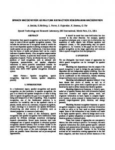
in which {s(1), . . . s(T )} denotes the temporal alignment of acoustic units associated with sub-word unit sequence U 1 . The left-hand side of Figure 1 illustrates frame-based recognition. While the frame based modeling offers an elegant probabilistic model that lends itself to a relatively simple implementation, the unrealistic frame-by-frame independence assumption is a major concern. Segmental methods have been proposed as a way to overcome this frame-by-frame independence assumption. In order to accommodate a model where multiple frames dependencies can be captured, segment based models introduce an unobservable segmentation variable S such that p(X|U ) can be represented as

k ... kcl

aa

states

... “dark” ...

language model

ah

states

Pronunciation model

ax

decoding frames

segments

p(X|U ) =

recognized utterance multi-dimensional frame

segment boundaries

units U representing (context-dependent) phones or some other linguistically inspired units [12]: = =

arg max W

arg max W

X

P (W, U |X)

U

X

p(X|U, W )P (U |W )P (W )

(1)

U

The latter expression was obtained by the application of Bayes rule and the observation that the maximization is independent of the observation likelihood p(X). In Eq. 1, since only subword units U that are a representation for W have a non-zero probability P (U |W ), we can rewrite Eq. 1 as X ˆ = arg max W p(X|U )P (U |W )P (W ) (2) W

X S

Fig. 1: Frame and Segment Based Recognition

ˆ W

(3)

ah kcl k

segments

dh

p(x(t)|s(t))P (s(t)|s(t − 1))]

{s(1),...,s(T )}

(1)

weights

segments

X

p(X|U ) = [

U

which conveniently factors into 3 components: the language model P (W ), the pronunciation model P (U |W ) and the acoustic model p(X|U ). It is the acoustic model which links observations to acoustic units that is the focus of this paper. Frame and Segment Based Models Most ASR systems are frame-based, in which observations X are a temporal sequence {x(1), x(2) . . . , x(T )} of acoustic feature vectors computed at regular time intervals, typically every 10 ms. Hidden Markov Models (HMMs) are a popular methodology to model acoustic units in a frame-based system. In a frame-based HMM system, we assume that X is a random process generated by an HMM whose states {s(1), s(2) . . . , s(T )} are the unobserved states of the Markov chains of a given acoustic unit sequence U . We typically make a first order Markov assumption between states s(t) and s(t − 1), and also assume a frame-by-frame independence assumption between observations x(t) and x(t−1). As a result, the acoustic model P (X|U ) can be written as [12]:

p(X, S|U ) =

X

p(X|S, U )P (S|U )

(4)

S

Intuitively, each segment spans multiple frames and is associated with one sub-word unit. This allows for modeling the dependency of multiple frames in each segment and only using the independence assumption at segment boundaries. The right-hand side of Figure 1 illustrates segment-based recognition. Implementing segmental models requires an approach to deal with the combinatorial size of the possible segmentations. This is achieved by only keeping a small number of segmentations to be used in the summation in Eq. 4 (or a Viterbi version where the best segmentation is selected). One approach to define segments is to perform a first pass HMM frame-based decoding, and define segments from the sub-word unit transitions in competing decoding hypotheses [13]. Alternatively, segments can be found by looking at large spectral changes in frame-level observations X [14]. A variety of methods have also been explored to model the probability p(X|S, U ). A first approach exists in using state trajectory modeling in which p(x(t)|s, u) is made dependent on the position of x(t) within the segment s spanning unit u. This approach still has a lot in common with HMMs as the acoustic model likelihood is computed as an accumulation of individual frame-based scores. At the other end of the spectrum are approaches that evaluate p(X|s, u) by first converting the variable length sequence of observations spanning over segment s to a new segmental feature vector [14], which has the potential to capture segmental characteristics. Global-Data vs. Exemplar-Based Models Independent of the exact nature of a speech recognition system, frame based or segmental, HMM or not, virtually all systems have in common that their acoustic models are global-data models, i.e. they build a single model to represent all data. The underlying computational engine may be e.g. Gaussian Mixture Models (GMMs), Neural Nets (NNs) [15] 1 In the remainder of this work, we use q when referring to generic acoustic classes, including units and HMM-states.

SAINATH ET AL.: EXEMPLAR-BASED PROCESSING FOR SPEECH RECOGNITION

or Support Vector Machines (SVMs) [16]. The speech signal that is fed to the recognizer is the result of a complex process governed by many inter-dependent phenomena such as gender, dialect, environmental noise, mood of the speaker, etc. To be computationally tractable, the global models for speech recognition must simplify the process by making questionable assumptions of independence. Hence, deriving a single global model relies on the assumption that averaging across training examples, across conditions and across all dimensions of the feature vector results in an average representation that is still reliable. This is questionable at least for two reasons [1]. First, there is evidence that a lower dimensional representation of speech feature vectors is possible than is suggested by the representational feature dimension which is around 40 for frame based systems [17] and significantly higher when considering stacks of consecutive frames [18]. The implied data sparseness requires prohibitively large databases for adequate model training such that in practice large portions of the representational feature space will inevitably be poorly modeled. It has been shown that in such situations exemplarbased methods that build local models can do a better classification job [19] and can do so in the original representational space [20]. Second, when few examples in the training data exist for a specific class, model parameters estimated for this class can be unreliable. Compensating for such data sparseness would likely require prohibitively large databases, at which point training the model would become computationally intractable. However, because exemplar-based techniques build local models using few relevant training examples, they do not suffer from data sparsity issues. It is our assumption that these two properties of exemplar-based techniques apply to the speech recognition problem both at the frame and the segment level. Evaluating Acoustic Models The ultimate evaluation of an acoustic model needs to happen in the context of a complete speech recognition system as in Eq. (2). Such experiments are tedious as they are typically run on very large databases that require the development of high quality linguistic components and interactions between the different components in the system may be hard to analyze. Therefore restricted experiments, such as phone recognition, which involves identifying phonemes (sub-units of words) from utterances, have been a popular alternative. Phone recognition involves only acoustic and language models. An even more restricted, and admittedly somewhat artificial, setup is phoneme classification in which an a priori segmentation of the data into acoustic units is given, and the goal is to classify segments into phonemes using only an acoustic model. III. T ECHNIQUES A. Overview The process of recognizing speech using exemplar-based techniques is illustrated in Fig. 1. The first step is to select appropriate acoustic features: feature extraction. Similar to other classical pattern recognition problems, it has been found beneficial to apply a feature transformation such as Principal

3

ACOUSTIC FEATURES FRAME-BASED

EXEMPLAR SELECTION

local pointwise matching in acoustic feature space

TEMPLATE-BASED

local trajectory matching in acoustic feature space

RELEVANT SUBSET

train

test

subset

Fig. 2: Overview of Exemplar Selection

Component Analysis (PCA) [21] or Linear Discriminant Analysis (LDA) [22] prior to exemplar-based processing. Apart from projecting into a space where a simple distance metric can be used to give a good notion of which exemplars are local to one another, such a feature transformation can reduce the influence of noisy and irrelevant features. It should be noted that PCA/LDA transformations are often applied to features irrespective of the modeling technique used (i.e., globaldata or exemplar-based). While these dimensionality reduction techniques throw away information in features, when applying a subsequent modeling step to these features, exemplar-based methods preserve information about individual features and dimensions better than global-data methods, as argued in Section II. The resulting training and test feature streams may or may not have associated segment boundaries. Referring back to Fig. 1, the acoustic evidence available in the feature space may therefore take the form of individual vectors, as in the frame-based path, or variable-length segments, as in the segment-based path. Depending on the choice of acoustic units, the acoustic inventory may thus be composed of fixedlength feature vectors (frames), or variable-length sequences of such vectors (templates). As mentioned earlier, segmental processing may also be done by integrating the variablelength sequence information into a fixed-dimensional feature vector by applying a suitable predefined warping function, for example by averaging and stacking consecutive frames [14]. Once the features have been defined, speech recognition typically entails three stages: exemplar selection, instance modeling, and frame- or segment-based decoding. 1) Exemplar Selection: Exemplar selection, detailed in Fig. 2, identifies instances from the training data which are most relevant to each test instance at hand. Such selection can be done in two steps [23]: first the training set is selectively downsampled to simplify the search, and then appropriate exemplars are taken from this reduced set. Either step may include exploiting any available prior knowledge about the task domain and/or test conditions. 2) Instance Modeling: In the second stage, the set of training instances identified via Step 1) as most relevant for the test instance at hand is used to model the test instance. Conceptually, this amounts to estimating a weight distribution characterizing the fractional contribution of each training exemplar to the test instance. In practice, this weight

4

distribution is primarily influenced by local acoustic information. In frame-based processing, this leads to techniques such as k-nearest neighbors (k-NN) [24] where prediction is directly restricted to a small number of nearest neighbors, or sparse representation (SR) approaches [23], [25], where prediction is more finely controlled via sparsity constraints. The same modeling techniques apply to segmental processing with fixed dimensional representation. In addition, in templatebased processing dynamic time warping (DTW) is used to compare variable-length sequences of frames [11], [26]. As discussed in Section II, in all cases exemplar-based techniques lead to representing each test instance in terms of a small number of selected training instances. 3) Frame- or Segment-based Decoding: Finally, the third stage involves recognizing an entire test utterance. Specifically, given the observation X, the instance models from Step 2), and a set of sub-word units U , an acoustic score p(X|U ) is computed directly for the segmental approaches or as outlined in Eq. (3) for the frame-based techniques. Based on the acoustic model score, along with the pronunciation model P (U |W ) and language model P (W ), a Viterbi search is performed to find the best set of recognized words, as in Eq. (2). The remainder of this section introduces various exemplarbased techniques, which differ in the definition, generation, and usage of their exemplars. It is important to note that these techniques are not always interchangeable: often one will be more appropriate to a particular situation than another. This explains why they have been more naturally deployed, at least initially, in different applications such as classification, recognition, and noise robustness. k-NN, briefly reviewed in Section III-B, is a basic technique that is applicable both in frame and segment-based processing. Others vary in terms of the number and length of the exemplars used. Methodologies typically involving fixed-length training instances include SR approaches, further discussed in Section III-C. Methodologies typically involving variablelength reference templates include template-based methods, which are described in detail in Section III-D. In between the extremes of frame-based processing and segment-based processing with predefined segments (typically phones), it is possible to exploit an inventory of data-driven acoustic segments, as exemplified in Section III-E. Finally, this section concludes with a summary of the salient commonalities and differences between the techniques in Section III-F.


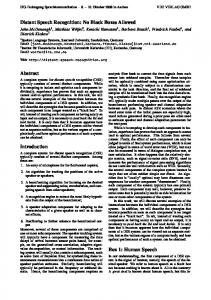
a brute-force approach, the reader is referred to [31] and the references therein. As an example, Fig. 3 shows the k = 13 nearest neighbors of an observed feature vector x, with both observation and exemplars represented with D = 2-dimensional features and a dotted circle visualizing an Euclidean distance metric. The N exemplars in the training set are collected in a D × N matrix H, with exemplars as its columns and each exemplar described by a D-dimensional feature vector. 2) Instance Modeling: In order to extract information useful for speech recognition or classification, exemplars are associated with labels. Labels can range from HMM-states on individual frames [27], to phone classes for phone segments [14], [29] and word labels for word segments [30]. Let there be Q classes. In the example of Fig. 3, Q = 3 and the Q × N matrix G is a binary matrix that associates each exemplar in H with class labels. Using a N -dimensional indicator vector i(C) containing ones for the indices c ∈ C and zeros otherwise, a k-NN based estimate of the class posteriors can be made as: pˆ(q|x) ∝ gq i(C). Here, gq represents the row in G corresponding to class q, effectively picking out those exemplars associated with that class. In weighted kNN, the binary values in i(C) are replaced with some weight representing the merit of each selected exemplar, for example derived from the distance of the exemplar to the test point. 3) Decoding: Classification is performed by empirical maximum likelihood (majority vote) [29]. For speech recognition, the posterior estimates Pˆ (q|x) need to be converted to frame-based observation likelihoods for use in (3). If x represents an individual frame the posterior estimates Pˆ (q|x) can be normalized to sum to one and then used directly as a value proportional to the observation likelihoods p(x|q), optionally after compensation for the class priors [27]. If x represents a fixed-length sequences of multiple frames, a sliding-window approach can be employed with averaging over overlapping posterior estimates [25], [28]. If an a-priori segmentation is available, one can perform segment-based decoding [14], with likelihoods obtained from segment-based posterior estimates or by averaging framebased likelihoods across all frames in a segment [14]. Alternatively, frame or segment based class posteriors can be converted to observation likelihoods by treating them as features in a discrete error model [32] or in a parametric model such as a GMM [33]. C. Sparse Representations

B. k-NN Classification 1) Exemplar Selection: The k-nearest neighbor (k-NN) algorithm is an algorithm which classifies a test point based on the identity of its k closest neighbors in the training set. Given a suitable distance metric d(·), k-NN can be used with exemplars of individual frames [27], fixed-length sequences of multiple frames [28], segments resampled to a fixedlength [14], [29] or even variable length segments [30]. In the exemplar selection step, a set C containing the indices of the nearest k exemplars is obtained. For an overview of techniques used to find the k nearest exemplars faster than

In recent years, sparse representation (SR) methods, perhaps best known from their use in compressive sensing (CS) [34], have become popular for pattern recognition tasks. Unlike k-NN, which explains a test point by a set of (individual) nearest neighbors, SR represents it as a linear combination of dictionary atoms. The most common applications of SRs is in signal compression and reconstruction, where the dictionary obeys a restricted isometric property (RIP) [35] and is nearly orthornormal. Recently, SRs have been used in classification tasks [2], with dictionaries constructed from examples of the signal, thus providing an exemplar-based representation. SR


dim2

Reference points (training data) label=A label=B label=Z

5

Test point (observation x ) k nearest neighbours classification: majority vote prob. estim. : rel. freq.

H=

(0.5,0.9)

(1.3,0.4)

G=

(0.2,0.3) (0.1,0.2)

0.1 0.2 ... 1.3 ... 0.5 ...

dim1

0.2 0.3 ... 0.4 ... 0.9 ...

dim2

1 0 0

1 ... 0 ... 0 ... 0 ... 1 ... 0 ... 0 ... 0 ... 1 ...

A B C

dim1

Fig. 3: An example of k-NN operating in a two-dimensional feature space. In the left panel the distance between an observed feature vector x and a set of exemplars are shown, and in the right panel the mathematical description of the exemplars and the exemplar-label association, H and G respectively, is visualized. The columns of H and G correspond to the exemplars in the left panel.

can be used with exemplars of individual frames [17], [36], fixed-length sequences of multiple frames [25], [28], [36] and with segments resampled to a fixed-length [29]. 1) Exemplar Selection: The SR β of the fixed-length observation x is obtained by finding a linear combination of exemplars that accurately describes x, i.e., x = Hβ, with H introduced in Section III-B. If the size of the dictionary H is large, the subsequent optimization problem can become computationally unfeasible. In that case, H can be limited to a subset of the complete training set, for example derived through random subsampling [25], [36], or on-the-fly by preselection with a search based on k-NN [17]. Ideally, the optimal β is sparse since only the atoms in H which belong to the same class as x should have a nonzero activation [2]. There is a vast literature discussing under which conditions SRs exist, given x and H, and discussing approaches to efficiently find these SRs — the reader is referred to [34], [37], [38] and the references therein. In the context of exemplar-based speech recognition, solving for β has been done for example by means of Lasso [40], which minimizes the Euclidean distance [39] while enforcing sparsity using an L1 constraint on β. Other distance metrics and techniques can be used as well. In [25], the Kullback-Leibler divergence was employed as distance metric. In [29], β was found by means of Sparse Representations via a Convex-Hull, employing regularization using a combination of L1 and L2 constraints to encourage the selection of groups of variables (group sparsity). 2) Instance Modeling: Although there are alternatives [17], the most straightforward method to recognize or classify test instances with SRs is analogous to the approach in Section III-B: a label matrix G is used to associate exemplars with class labels, and posterior estimates are obtained as Pˆ (q|x) ∝ gq β. In [33], the posteriors represent phone classes and are referred to as Sparse Representation Phone Identification Features (Spif ). In [25], the posteriors represent HMM states and the use of these posteriors in a hybrid SRHMM recognizer is referred to as Sparse Classification (SC). 3) Decoding: Classification and recognition are largely analogous to the approaches described in Section III-B3:

classification can be performed by selecting the class with the empirical maximum likelihood and for recognition posterior estimates Pˆ (q|x) can be converted to frame-based observation likelihoods for use in (3). Alternatively, one can construct ˜ = Hβ and train a GMM to convert these a new feature x features to observation likelihoods [17]. Intuitively, the feature ˜ can be thought of as mapping the test point back on the space x spanned by the training examples. These features can be used for both frame and segment-based decoding. 4) Noise robustness using sparse representations: Over the past few years, it has become clear that SRs employing exemplars as dictionary atoms can be an effective approach for noise robust ASR. There are two methods that have employed exemplar-based SRs for noise robust ASR, and they both work by modifying the exemplar-selection process so that SRs are obtained that are invariant under additive noise. The first method is a missing data technique [40] dubbed sparse imputation [36], which operates under the assumption that even in noisy speech, certain log-compressed Mel-spectral noisy speech features stay relatively uncorrupted. After identifying the corrupted features, one estimates (‘imputes’) clean speech estimates for these features (‘feature enhancement’). Mathematically, for each observation x a missing data “mask” m is defined, which is a binary vector that labels the uncorrupted dimensions in x as one, and the noise-corrupted features with zero. A SR is obtained by solving Wx = WHβ with W a diagonal matrix with the mask m on the diagonal. Feature enhancement (FE) is performed by calculating the ˜ = Hβ, after which these features can be reconstruction x used in a conventional GMM/HMM system. The second method is based on source separation: a noisy speech observation x is described as a linear combination of a clean speech dictionary Hs and a noise dictionary Hn : x = Hβ = [Hs Hn ]β [25]. This does require that x is based on a representation in which noise and speech add (approximately) linearly, such as for example the Mel-magnitude domain. The reader is referred to [41]–[44] and the references therein for an overview of related methods, although most of these do not employ exemplars as dictionary atoms and focus on source separation rather than noise robust ASR.

6

After obtaining the SR, noisy speech can be recognized or classified using the techniques described in Section III-C2, with the only difference that βs , corresponding to activations of the speech dictionary Hs , is used instead of β [25]. Alternatively, one can do FE by making the clean speech ˜ = Hs βs [25]. reconstruction x D. Template Matching In the template matching approach, the acoustic model is implemented by means of a non-parametric method which compares reference templates directly with the observed features X. The reference templates here are chunks of audio drawn from the training database that act as exemplars for a certain acoustic unit u. An important difference between the template matching approach and the previously described exemplar-based methods is the use of variable length units, and hence the need to compare trajectories with DTW. The template matching system typically starts from a pre-existing word/phone graph in order to keep the number of candidate segments and corresponding class labels manageable. This graph can for example be made via quick and approximate template matching techniques [45] or via a classical HMM system [46]. 1) Selection: Fig. 4 illustrates a template matching setup in which a standard HMM system first generates a graph containing the most likely words given the speech signal. Each word arc is augmented with its underlying sub-word segmentation (phone identities plus begin and end times) to allow for template matching based on sub-word units (cf. section II). The next step consists in computing exemplar-based scores for all (sub-)word arcs, after which a second decoder finds the best word sequence in the graph according to (2). In order to derive a score p(X|u) for a (sub-)word arc, the set of k templates drawn for the training database that (1) match the (sub-)word identity u, and (2) resemble the sequence of acoustic features observed for that (sub-)word arc X as well as possible, are collected. 2) Modeling: Since variable length segments need to be compared, time warping/alignment is needed. Allowing little to no time warping during the comparison would require a huge training database containing speech at all possible speech rates. On the other hand, giving the system lots of freedom during the alignment would allow for unnatural time warping curves. Experiments have showed that constrained Dynamic Time Warping (DTW) offers a good compromise [47]. When comparing trajectories, DTW basically sums up distances between individual frames. Hence, the same feature preconditioning techniques as described in section III-A may be applied. The preconditioning should befit the distance metric used to compute the local distances. For example, the commonly used Euclidean distance makes the implicit assumption of uniform variances across all classes and thus the preconditioning should try to achieve this. Since feature preconditioning is applied globally, residual differences between class variances are unavoidable. Hence, the local distances can be improved upon by introducing variances in the distance


measure. These variances are either determined based on the acoustic class q the reference frame belongs to [45] or estimated based on the location of the test observation x in the feature space [47]. 3) Single Best Decoding: Template matching by means of DTW can be viewed as an extreme variant of the segmental mixtures of discrete non-parametric trajectory models described in [48], a variant in which each exemplar forms a trajectory on itself. This analogy is further explored in [45], starting from the link between non-parametric density estimation techniques such as kernel/Parzen estimates [49] and the local distance measure used in DTW. This leads to the observation that DTW distances can be directly related to the segment log-likelihoods log p(X|u) and hence can be plugged into Eq. (2). This results in a single best decoder which finds the string of best matching exemplars along with the recognized word string. Such a single best template-based decoder is sensitive to inaccuracies in the training database such as faulty phone labels due to non-standard word pronunciations. This can be effectively remedied by means of “data sharpening”, a technique that implicitly finds outliers and adjusts their feature vectors so that they are more representative of the class they belong to [50]. The accuracy of the decoder can be improved further by promoting natural and smooth transitions at template boundaries, i.e. the complete sequence of templates chosen to explain a sentence should not show odd discontinuities in the feature vector values around template transitions. This can be obtained with transition costs [45], context-dependent templates [46] or by favoring signal continuity across template boundaries [47]. Another technique is to employ longer span acoustic units such as word templates when sufficient examples are available with a back-off to syllable or phone templates for words which are missing or are found only a few times in the training data [47]. 4) Decoding via weighted k-NN: Instead of relying on the score of the single best template only, a decoder could also first derive more robust ensemble scores, i.e. a weighted sum of the k best DTW scores, similar to what is done in the k-NN method (Section III-B). As is shown in [47], the techniques mentioned above can be adapted to this framework. In addition, the selected k-NN templates can be readily queried about relevant properties of the (sub-)word arc under investigation, be it at the signal level or with respect to some additional meta-information that is stored with the labels [30]. Relevant meta-information are properties that can help in confirming or denying the word hypothesis built on top of the phone, syllable or word arc for which the k-NN templates were searched for. Some examples thereof are: • Is the phone a word initial, word final or word central phone, and does this correspond to its use in the word hypothesis? • From which words are the phone exemplars drawn, and is this consistent with the word hypothesis? One advantage of inferring this information via k-NN is that multiple properties can be queried simultaneously without subdividing the training data in increasingly smaller classes and hence avoiding data sparsity.


SEIB 81.69

HMM system

1.05

AND -11.01

SEA 64.66

q1

q2

q3

BUT 15.29

SEE 64.66

word graph + phone segmentation

SEE 45.87

0.99

BET 37.82

E. 1.50

THAT 15.65

C. 45.87 SEE 57.42

1.00

C. 57.42

0.72

SEED 59.05 1.4

SEIB 77.82

0.4

phone labels

0.2

begin/end time

kHertz 0

5

0

optimal path (alignment) start5

kHertz

pre−segmented + labelled train database

1.05

0.6 0.8 Seconds

1

SEIB 79.87

0

kNN templates 0

0.5

1

TO 23.82

1.52

TO 25.23

AGREED 62.05 AGREED 68.46 A 15.26

A -4.23

1.04

AGREED 63.74

AGREED 63.28

CIBA 86.88 1.20

1.61

1.48

AGREE 57.32

1.07

CIBA 73.59

acoustic features distance matrix

1.2

reference template (phone/word segment)

end

Dynamic Time Warping (DTW)

1.03

1.20 1.21 THAT 17.10 THE 11.06

THE -8.06

SEA 57.42

DTW−kNN search

BUT 13.66

E. 10.25 0.93

SEA 45.87

AGREED 69.01

1.14

C. 64.66

A 7.02

word arc (from a word graph) agreed underlying phone arcs / / /g/ /r/ /i:/ /d/ expansion into k template arcs (nearest neighbours) e

audio

7

...

...

...

...

...

1.5

hypothesizedSeconds phone/word arc

combine scores

rescore word graph

Fig. 4: A possible template matching setup.

Combining the multiple k-NN scores with the word and phone based weighted DTW-scores requires a decoding strategy that can effectively integrate multiple and heterogeneous information streams. In [30] this was accomplished with Segmental Conditional Random Fields (SCRFs). E. Latent Perceptual Mapping Latent Perceptual Mapping (LPM) is related to both SRs and template matching, but it exploits a different representation of the acoustic evidence available and operates with data-driven acoustic units [51]. The underlying motivation is to find recurring patterns (templates) that help characterize different phone classes. This motivation is shared with Van hamme’s histogram of acoustic co-occurrence model [52], where hidden structure in speech utterances is also exposed through recurring acoustic patterns. LPM closely parallels latent semantic mapping (LSM) in text indexing and retrieval [53], where a text document is treated as a bag of words. In the same way, in LPM a speech segment (e.g., phone or supra-phone segments) is treated as a bag of acoustic units drawn from a limited acoustic vocabulary. Supra-frame information is incorporated by considering (variable-length) multi-frame sequences of feature vectors. This leads to a description of each speech segment as a bag of units. Next, a subset of the units is selected as templates, and weighted frequency counts between segments and templates are computed to generate a segment-template co-occurrence matrix. A singular-value decomposition (SVD) of this matrix creates a new latent feature space, spanned by the left and right singular vectors. Both segments and templates are represented by reduced-dimensionality vectors in the latent space. Classification is then performed by mapping test segments to the latent space. The process is illustrated in Fig. 5. Depending on the acoustic units (single or multiple frames) selected as templates, LPM is applicable to both framebased and segment-based processing. In contrast with previous techniques, the LPM segment-template matrix can thus encode

both frame-based and supra-frame (template-based) information for a given speech segment. In this framework, the (initial) selection step is thus closer to pre-selection in other exemplarbased techniques, in that an initial set of templates must be defined a priori in order to construct the latent space. Once the representation of a test instance is available in that space, however, it becomes possible to refine the set of templates on the basis of that test instance, leading to a revised segmenttemplate matrix specifically tailored to the observation at hand. This in turn leads to a new latent space better suited to the test segment. In other words, LPM normally involves several selection/modeling iterations. 1) Selection: In order to derive an initial set of data-driven (fixed- or variable-length) templates, feature vectors associated with M training segments are first vector quantized using a codebook obtained by unsupervised clustering. The resulting sequences of symbols are then broken into n-gram units (1 ≤ n ≤ 20), where longer units intrinsically incorporate supra-frame level temporal information. Depending on the value of n, LPM thus accommodates single-frame units and longer templates. Pre-selecting longer templates directly (e.g., by using local trajectory matching) proves computationally intractable, however, as the number of n-gram templates can be much larger than the number of feature vectors available for training. This is solved by sub-sampling the n-gram templates so that the most informative ones are retained based on their indexing power [53]. The outcome is a set of N relevant templates, which serve as columns for a M × N segmenttemplate co-occurrence matrix F. Entries of this matrix are calculated by counting the number of times each template appears in each speech segment [54]. This is obtained by finding the nearest template for each unit of a given segment (using either k-NN or DTW depending on unit length) and incrementing the count of the column entry associated with that selected template. Thereafter, a reducedrank approximation is obtained via singular value decompo˜ M ×N = UM ×R · ΣR×R · V T , sition (SVD) as follows: F N ×R where R approximates the rank of F (R ≤ min(M, N )). The observed acoustic evidence is now encapsulated in the vector

8


cluserting

quantization

selection uttr 1 uttr 2 uttr M

ﬁxed / variable length units

templ: templates

N templ S

VT

U MxN

N templ

test uttr

F. Commonalities and Differences

similartity

TEST feature extraction

TRAINING feature extraction

codebook

VT

class label

1xN

Fig. 5: Latent Perceptual Mapping for Classification

space of dimension R spanned by the singular vectors. Since the mth segment in the collection is characterized by the mth ˜ the row vector ym = um · Σ characterizes the row of F, position of this segment in the latent space. 2) Modeling: Similarly, an unknown segment is mapped onto the space using the “folding in” approach described in [53]. Given the N relevant templates and the right singular vectors of the SVD, a test segment X is mapped as yx = fx ·V, where fx is the segment-template vector associated with this test segment. A k-NN rule is then used to produce a local, exemplar-based model for the observed acoustic information. Note that the derivation of fx and its mapping to the space intrinsically unifies both single- and multi-frame distance metrics in a joined (typically cosine-based) measure in the latent space [51], [53], [54]. Because the latent space comprises both segments and templates, this local model can be exploited in two ways: (i) if selecting training segments similar to the test instance, these exemplars can inform a new template selection process that is better aligned with the observation; and (ii) if selecting templates similar to the test instance, the selected templates can reveal specific characteristics (e.g., in terms of common length or shared frame sub-sequences) that can help select a more relevant set of templates in the segment-template matrix. In either case, the outcome is a new latent space better tailored to the test instance at hand (and often of lower dimensionality), in which a new local model can be computed. 3) Decoding: This local model is used in a straightforward manner to predict the class label of X. As with other exemplarbased methods, this approach can be extended to recognition problems by feeding segment class labels to sequential modeling techniques such as HMMs or SCRFs. Interestingly, from two different angles LPM and SR both achieve a parsimonious representation of the acoustic information. The number of units N in LPM is somewhat analogous to the number of retained exemplars in SR, and the vector yx in the latent feature space plays the same role as Hβ in SR. The same way the weight vector weighs the “best” instances in the dictionary H to represent the data, LPM represents each observation as a linear combination of the “best” data-driven templates obtained as projection into the latent perceptual space. This illustrates the duality of parsimoniousness as dimensionality reduction and sparsity.

1) Selection: The k-NN approach requires a test instance to be compared with all training instances, possibly using approximate search techniques to reduce computational effort. All other exemplar-based techniques operate on a subset of relevant training instances according to the location of the test segment in the feature space. Sparse representation methods use k-NN or random sampling to pre-select appropriate instances, so as to efficiently generate local posteriors. Template matching uses the initial word graph first to limit the number of possible classes (and segment boundaries) and uses k-NN to sub-select templates within the classes. Latent perceptual mapping uses clustering and pruning to sub-sample appropriate templates for building the segment-template matrix. 2) Instance Modeling: All exemplar-based techniques rely on a parsimonious matching of acoustic units, from single frames (in the case of frame-based processing) to complete phone segments (in the case of template-based processing). Here we use the term parsimonious to refer to the fact that only a few elements (or dimensions for LPM) are needed to uniquely represent acoustic units. The number of acoustic units varies from the number of segments available (in the case of template-based processing) to the total number of feature vectors extracted (in the case of frame-based processing). Both k-NN and SR operate on fixed-length frames, though SR may also be extended to fixed-length sequences of frames. By considering variable-length sequences of frames, DTW techniques are able to explicitly cope with temporal variations in speech. LPM can operate on either type of acoustic units. By restricting the length of the units to single frames, and considering all frames in the training data, LPM acts as a kNN approach [51]. In contrast, by restricting the length of the acoustic units to complete phone segments, LPM leads to a DTW-like template comparison approach [55]. 3) Decoding: Just like classical HMM methods, DTWbased template matching techniques calculate the class conditional likelihoods p(x|q) used for recognition. In contrast, kNN and SR calculate the local posterior Pˆ (q|x) of an unknown test utterance, and converted into likelihoods as described in Section III-B3. Alternatively, local posterior probabilities, or the reconstructed utterance Hβ in SR can be used as a feature to train GMMs and incorporate into a standard GMM/HMM framework. As mentioned above, Hβ could also be replaced by the dimensionality-reduced expression fx V from LPM. IV. E XPERIMENTAL R ESULTS A. Overview Exemplar-based techniques have been applied to both classification and recognition problems, as well as more generally to achieve noise robustness. The goal of this section is to highlight some of the improvements that have been observed in terms of a reduction in error rate. Not surprisingly, most results reported in the literature are not directly comparable, because of different tasks, different corpora, different feature extraction, and/or possibly different randomized and irreproducible splits of training and test data. Thus, the aim is not to compare exemplar-based techniques to each other, but rather to


some established baseline appropriate for the task considered. In most cases, this baseline corresponds to a state-of-the-art implementation of the best “classical” (non-exemplar-based) approach available. Speech research in classification is most often explored on TIMIT [56], a small vocabulary acoustic phonetic task. TIMIT provides standardized training, development and test sets, as well as time-aligned phonetic transcriptions. These benefits of TIMIT have made it possible to easily compare different methodologies on one unified task, making it a benchmark data set for classification experiments in the speech community. Results with exemplar-based methods on TIMIT are reported in Section IV-B. Recognition tasks involve the added challenge of integrating local posterior scores across frames and thus typically necessitate a larger amount of training data. Characterizing a test sample by searching over such a large amount is computationally expensive relative to evaluating a set of Gaussian mixtures. Therefore, work with exemplar-based methods started on small vocabulary tasks i.e., tasks where all utterances can be formed from less than 5,000 distinct words. Small vocabulary tasks allow new research ideas to quickly be tested before exploring the same ideas on larger tasks. Recent advances in computing power and storage have made exemplar-based approaches more computationally feasible allowing for exploration on larger vocabularies. In addition, improvements in machine learning algorithms have led to improvements in the methods themselves, thus enabling large vocabulary continuous speech recognition (LVCSR) tasks—with over 20,000 words. Related results are reported in Section IV-C. Finally, exemplar-based techniques have also been applied to the problem of noise robustness, either via sparse imputation or source separation, as discussed in Section IV-D. B. Classification This section presents classification results using exemplarbased methods. 1) Template Matching: Early success with exemplar-based methods was presented in [57] on TIMIT . Using simple MFCC features, a classification error of 20.7% was achieved using DTW scores followed by a k-NN classifier; while using the same features in a GMM classifier achieves 21.6% classification error. One striking observation is the importance of data sharpening to remove outliers [50], which contributed roughly 3.0% absolute to the template matching results. 2) SR: SRs using more sophisticated speaker-adapted, discriminatively trained features were explored in [29]. Table I compares the classification error of the SR classifier to many standard classifiers used on this task, including a GMM, SVM and k-NN classifier. First, notice that both exemplar-based classifiers, namely SR and k-NN, offer improvements over the pre-existing global-data modeling techniques, namely GMM and SVM. While k-NNs characterize a test point by selecting a small and fixed number of k neighbors from the training set, SRs do not fix the number of neighborhood points chosen in training, and appear to be more robust classifiers. The SR method achieves a classification error of less than 15%, the best classification result reported on TIMIT to date.

9

TABLE I: Classification Error, TIMIT Core Test Set Method Accuracy

GMM 17.2

SVM 17.4

k-NN 16.4

SR 14.9

3) LPM: Early experiments with LPM conducted on focused on dimensionality reduction rather than accuracy improvements. By retaining only 10% of the maximum dimensionality of the latent space, frame-based LPM operating on vector-quantized phone segments scored at the level of both DTW and discrete-parameter HMM systems [51]. By incorporating supra-frame information [29] and increasing the dimensionality, LPM could reach the performance of a continuous-parameter GMM/HMM system. On the other hand, template-based LPM using short, variable-length units (1- to 3-grams) [55] achieved the same level of performance at a dimensionality less than or comparable to that of the original acoustic space (40). This is in contrast with direct DTW, where the corresponding dimensionality is the total number of TIMIT training phone segments (about 140,000). In addition, longer templates were observed to allow further dimensionality reduction (down to less than 10), which suggests that in LPM parsimoniousness hinges on the interplay between dimensionality and unit length. TIMIT

C. Recognition 1) k-NN: Several authors have taken the approach of converting the weighted distance measured by a frame based kNN classifier to an HMM observation probability. In [27] the authors show that on a small vocabulary continuous digit task the k-NN method is comparable to a GMM/HMM-based approach. However, on a large vocabulary English transcription task, the authors show that the nearest neighbor method is only able to offer improvement over the GMM/HMM-based approach when less than 3 hours of training data is used. In [32] smoothing across frames is applied to generate more consistent observation probabilities leading to a 0.9% absolute improvement over a baseline GMM/HMM system with a word error rate (WER) of 35.4%. 2) Sparse Representations: The use of SR reconstruction features, referred to as Hβ, was first explored on the TIMIT corpus. In [17], the authors show that the Hβ features offer a phonetic error rate (PER) of 18.6%, a 0.8% absolute improvement over a state-of-the-art GMM/HMM system. In fact the PER of 18.6% is the best reported recognition result on TIMIT to date. After using TIMIT as a quick methodology to explore the benefit of the Hβ features, [17] investigates the performance of the Hβ features on a 50-hour LVCSR English Broadcast News task. Even on a larger task, the use of Hβ features provided a word error rate (WER) of 18.7%, a 0.3% improvement over a state-of-the-art GMM/HMM system, which is significant for this task. These experiments demonstrate that the benefit of Hβ features in mapping the test sample back onto the space spanned by the training examples, results in improvements in recognition applications. An exploration of the exemplar-based posterior Spif was explored in [23] on two LVCSR tasks, an English Broadcast News (BN) task with acoustic models trained on 50 hours of

10

speech data and a Voice Search (VS) task with acoustic models trained on 160 hours. The Spif features offer 0.6% and 1% absolute improvements on the BN and VS tasks respectively compared to a GMM/HMM system, demonstrating that even with large amounts of data these features are still able to capture the benefit of exemplar-based methods and provide improvements over a GMM/HMM system. Furthermore, in [23] it was observed that on even larger tasks with acoustic models trained on 400 and 1,280 hours, the use of Spif features still provided improvements over the baseline system. 3) Template Matching: Research into continuous speech recognition with template matching techniques was first explored on small vocabulary tasks such as Resource Management (RM). More recently, the focus has shifted to larger tasks such as the 20,000 vocabulary Wall Street Journal (WSJ) task with research continuing in the direction of large vocabulary broadcast news and telephone transcriptions. Given that template matching systems use the local distances directly in the computation of observation likelihoods, proper feature preconditioning and high quality local distance measures have proven to be very valuable: • feature preconditioning resulted in a 39% relative improvement on the RM task [58] • incorporating class variances in the distance measure resulted in an additional 39% relative improvement [58] • the use of data sharpening to remove outliers has shown consistent 10-25% relative improvements on a variety of tasks [46], [50]. Consistent improvements have also been observed by enforcing strong continuity constraints, not only within the templates themselves as DTW already does that implicitly, but also across templates by means of continuity constraints [46], [47]. On the RM task, a single best template sequence decoder [57] incorporating most of the above concepts, outperforms a comparable HMM based system (3.07% versus 3.35% WER). However, we must note that the RM task suits template based systems well by its relatively small vocabulary size (1000 words), assuring that there are ample examples for each required phone in context and even for each word. On the more complex WSJ task, the best results have been obtained when using weighted k-NN template distance scores in combination with a wealth of k-NN based metainformation all integrated in a Segmental Conditional Random Field (SCRF) decoder. The combination of score averaging, harvesting additional information via k-NN, and additional continuity constraints gave a 21% relative improvement on the task [30] which resulted in a 7.6% absolute WER, which is roughly on par with a comparable GMM/HMM system. On both the single best decoder and the DTW/k-NN systems, we observed that the template based systems often make mistakes which are quite different compared to GMM/HMM systems. On the one hand this illustrates the intrinsic differences of these methods versus HMMs. On the other hand, it makes template based systems ideally suited for combination with GMM/HMMs. Such combined DTW/HMM systems achieve the best published results obtained on both the RM and WSJ tasks.


D. Noise Robustness As described in Section III-C4, exemplar-based methods have been used to provide noise robustness for ASR using two different approaches. The missing-data based feature enhancement approach called sparse imputation (SI) is similar to the use of Hβ features. The second approach is based on source separation and can be used in two ways, either as a feature enhancement approach (FE) using Hβ features, or through a method known as sparse classification (SC). SC is conceptually similar to the use of Spif features, as this approach directly provides posterior HMM-state label estimates for use in a hybrid exemplar-based/HMM recognizer. 1) Sparse imputation: The exemplar-based missing data SI approach has been evaluated both on a classification task as well as on small and large vocabulary speech recognition databases [36], [59]. In these works, the performance of SI has been compared with the performance obtained with conventional missing data imputation methods (employing global data models) in two scenarios: one in which the missing data mask did not contain errors (the so-called oracle mask) and one in which the mask was realistically estimated from the noisy speech. It was observed that SI performed comparably to the conventional methods when using estimated masks, but performed much better when using oracle masks. For example, on the noisy digit recognition task AURORA -2 , SI employing oracle masks achieves an impressive 2% WER at SNR −5 dB, whereas conventional imputation methods only achieve 44% WER [59]. The reason for the success of exemplar-based methods is in large part due to the fact that global data noise robustness models operate on single time frames, whereas SI is able to exploit all the information contained in segments compromising many frames. 2) Source separation based approaches: The more recently introduced exemplar-based approaches FE and SC do not have the aforementioned sensitivity toward a missing data mask as they rely on source separation with both a speech and noise dictionary. In evaluations on small vocabulary recognition tasks [25], [60] it was shown that both the FE approach and the SC approach improve the noise robustness, with SC yielding higher accuracies than FE at low SNRs at the cost of lower accuracies at high SNRs. Although of course not as effective as SI using an oracle mask, both the FE and SC methods performed substantially better than SI employing estimated masks. Again, the fact that exemplars can accurately model the temporal context was shown to be very helpful in providing noise robustness at low SNRs: For example, on AURORA -2 SC achieves 37.6% WER at SNR −5 dB [60], whereas modern conventional noise robustness methods only achieve 53.8% WER [61]. A recent line of research in the community is combination of exemplar-based noise robust methods with conventional GMM-based recognition in a multi-stream architecture [62]. The results obtained in that work show that in such dualinput systems the noise robustness of SC at low SNRs is retained while achieving the same performance at high SNRs as obtained with global-data modeling.


V. C ONCLUSIONS AND F UTURE D IRECTIONS In this article, we have provided an overview of exemplarbased processing for speech recognition. Exemplar-based methods discussed in this paper, including k-NN, SR, DTW and LPM, differ in how exemplars are selected, instances are modeled, and sequences are decoded. We have shown how exemplar-based techniques for speech recognition can address deficiencies of global-data models like GMMs, SVMs, and NNs: whereas global-data methods introduce independence assumptions to keep the models computationally tractable, exemplar-based techniques, by building local models, can stay closer to the underlying speech production process, while at the same time keeping the number of parameters parsimonious. For example, fitting an approximate global model on the training data may lead to poor modeling of rare events, or equivalently, the need to increase the number of free model parameters (and therefore the amount of training data required to estimate them) in order to achieve a fine enough modeling. Exemplar-based techniques not only allow the modeling of fine details, they provide a way to simultaneously address the frame independence assumption and other independence assumptions of HMMs. This has allowed for success not only in speech classification, but also in small and large vocabulary speech recognition, and more generally in achieving robustness across a wide number of tasks. Several promising research directions are being actively pursued in exemplar-based processing. First, efforts are under way to improve every component in an exemplar-based system. For exemplar selection, it is important to make the local metric robust to known sources of variability in speech. For instance modeling, various methods are being investigated to improve inference from the selected exemplars, for example by looking at the distribution of exemplars around the test instance, or via better segment trajectory comparisons and/or combinations. For sequential decoding, tighter constraints should be incorporated into the search to ensure that any hypothesized exemplar sequence that cannot be produced by a human vocal tract is properly penalized. Second, given that all exemplar-based methods relate a test instance to a compact set of exemplars drawn from the training data, they inherently complement, in a robust manner, the information captured within global-data models. This has sparked interest in various combinations between the two approaches. For example, exemplar-based processing can easily generate features to be incorporated into Deep Belief Networks (DBNs) [63], or act as a posterior probability estimator that can be used as one of the experts in a committee-of-experts setting or maximum entropy framework [64]. Training samples judiciously selected via exemplar-based processing can also be used to advantageously augment a limited corpus available for a particular user, domain, or environment. More generally, exemplar-based processing could potentially support inference from any training corpus enriched with information not immediately usable by global-data models, such as prosody. Finally, it is critical to keep on improving the computational efficiency of exemplar-based methods, including searching for relevant exemplars in large data sets and quickly making clas-

11

sification decisions. With increased consumer use of speech recognition technologies, the size of datasets are expected to grow rapidly to tens of thousands of hours of data. Given on-going computational and machine learning advances, we believe this will allow exemplar-based methods to have a much larger impact on real-world speech recognition tasks. R EFERENCES [1] T. Mitchell, Machine Learning. McGraw Hill, 1997. [2] J. Wright, A. Y. Yang, A. Ganesh, S. S. Sastry, and Y. Ma, “Robust face recognition via sparse representation,” IEEE Transactions on Pattern Analysis and Machine Intelligence, vol. 31, no. 2, pp. 210–227, February 2009. [3] H. Zhang, “SVM-KNN: Discriminative Nearest Neighbor Classification for Visual Category Recognition,” in Proc. CVPR, 2006. [4] R. Brunelli and T. Poggio, “Face Recognition: Features versus Templates,” IEEE Transactions on Pattern Analysis and Machine Intelligence, vol. 15, no. 10, pp. 1042–1052, October 1993. [5] E. Wold, T. Blum, D. Keislar, and J. Wheaten, “Content-based classification, search and retrieval of audio,” Multimedia, IEEE, vol. 3, no. 3, pp. 27–36, Fall 1996. [6] S. Li, “Content-based audio classification and retrieval using the nearest feature line method,” IEEE Transactions on Speech and Audio Processing, vol. 8, no. 5, pp. 619–625, September 2000. [7] S. Sundaram and S. S. Narayanan, “Classification of sound clips by two schemes: using onomatopoeia and semantic labels,” in Proceedings of the IEEE International Conference on Multimedia and Expo (ICME), Hannover, Germany, June 2008, pp. 1341–1344. [8] Lee, K. and Ellis, D.P.W, “Audio-Based Semantic Concept Classification for Consumer Video,” IEEE Transactions on Audio, Speech and Language Processing, vol. 18, pp. 1406 – 1416, August 2010. [9] M. D. Plumbley, T. Blumensath, L. Daudet, R. Gribonval, and M. E. Davies, “Sparse representations in audio & music: from coding to source separation,” Proceedings of the IEEE, vol. 98, no. 6, pp. 995–1005, 2009. [10] Y. Panagakis, C. Kotropoulos, and G. R. Arce, “Music genre classification via sparse representations of auditory temporal modulations,” in 17th European Signal Processing Conference (EUSIPCO 2009), Glasgow, Scotland, August 2009, pp. 1–5. [11] M. De Wachter, K. Demuynck, D. Van Compernolle, and P. Wambacq, “Data driven example based continuous speech recognition,” in Proc. European Conference on Speech Communication and Technology, 2003. [12] F. Jelinek, Statistical Methods for Speech Recognition. MIT Press, 1997. [13] G. Zweig and P. Nguyen, “A segmental crf approach to large vocabulary continuous speech recognition,” in Proc. ASRU, 2007. [14] J. R. Glass, “A probabilistic framework for segment-based speech recognition,” Computer Speech and Language, vol. 2-3, pp. 137–152, April-July 2003. [15] N. Morgan and H. Boulard, “Neural Networks for Statistical Recognition of Continuous Speech,” Proc. IEEE, vol. 83, no. 5, pp. 742 – 772, May 1995. [16] V. Vapnik, The Nature of Statistical Learning Theory. Springer-Verlag, 1995. [17] T. N. Sainath, B. Ramabhadran, D. Nahamoo, D. Kanevsky, and A. Sethy, “Exemplar-Based Sparse Representation Features for Speech Recognition,” in Proc. Interspeech, 2010. [18] M. Nilsson and B. Kleijn, “On the estimation of differential entropy from data located on embedded manifolds,” IEEE Transactions on Information Theory, vol. 53, no. 7, Jul. 2007. [19] M. Belkin and P. Niyogi, “Using manifold structure for partially labeled classification.” in Advances in Neural Information Processing Systems, 2003, p. 929936. [20] P. Mordohai and G. Medioni, “Dimensionality estimation, manifold learning and function approximation using tensor voting,” Journal of Machine Learning Research, vol. 11, pp. 411–450, 2010. [21] I. Jolliffe, Principal Component Analysis. Springer Series in Statistics, 2002. [22] S. Mika, G. Ratsch, J. Weson, B. Scholkopf, and K. R. Mullers, “Fisher Discriminant Analysis With Kernels,” in Proc. of the 1999 IEEE Signal Processing Society Workshop, 1999. [23] T. N. Sainath, B. Ramabhadran, D. Nahamoo, and D. Kanevsky, “Reducing Computational Complexities of Exemplar-Based Sparse Representations With Applications to Large Vocabulary Speech Recognition,” in Proc. Interspeech, 2011.

12

[24] L. Golipour and D. O’Shaughnessy, “Context-independent phoneme recognition using a k-nearest neighbour classification approach,” in Acoustics, Speech and Signal Processing. ICASSP 2009. IEEE International Conference on, Taipei, Taiwan., April 2009, pp. 1341–1344. [25] J. F. Gemmeke, T. Virtanen, and A. Hurmalainen, “Exemplar-based sparse representations for noise robust automatic speech recognition,” IEEE Transactions on Audio, Speech and Language Processing, vol. 19, no. 7, pp. 2067–2080, 2011. [26] J. V. G. Aradilla and H. Bourlard, “Using posterior-based features in template matching for speech recognition,” in Prov. ICSLP, 2006. [27] T. Deselaers, G. Heigold, and H. Ney, “Speech Recognition With Statebased Nearest Neighbour Classifiers,” in Proc. Interspeech, 2007. [28] J. F. Gemmeke, L. ten Bosch, L.Boves, and B. Cranen, “Using sparse representations for exemplar based continuous digit recognition,” in Proc. EUSIPCO, Glasgow, Scotland, August 24–28 2009, pp. 1755– 1759. [29] T. N. Sainath, D. Nahamoo, D. Kanevsky, B. Ramabhadran, and P. M. Shah, “A Convex Hull Approach to Sparse Representations for Exemplar-Based Speech Recognition,” in Proc. ASRU, 2011. [30] K. Demuynck, D. Seppi, D. Van Compernolle, P. Nguyen, and G. Zweig, “Integrating meta-information into exemplar-based speech recognition with segmental conditional random fields,” in Proc. International Conference on Acoustics, Speech and Signal Processing, 2011. [31] H. Samet, “Similarity searching: Indexing, nearest neighbor finding dimensionality reduction, and embedding methods for applications in multimedia databases,” in Proc. International Conference on Pattern Recognition, 2004. [32] N. Singh-Miller and M. Collins, “Learning Label Embeddings for Nearest-Neighbor Multi-class Classification with an Application to Speech Recognition,” in Proc. NIPS, 2009. [33] T. N. Sainath, D. Nahamoo, D. Kanevsky, B. Ramabhadran, and P. M. Shah, “Exemplar-Based Sparse Representation Phone Identification Features,” in Proc. ICASSP, 2011. [34] E. J. Cand´es, , and M. B. Wakin, “An introduction to compressive sampling,” IEEE Signal Processing Magazine, vol. 25, no. 2, pp. 21–30, 2008. [35] E. J. Candes and T. Tao, “Decoding by Linear Programming,” IEEE Transactions in Information Theory, vol. 51, no. 12, pp. 4203–4215, 2005. [36] J. F. Gemmeke, B. Cranen, and U. Remes, “Sparse imputation for large vocabulary noise robust ASR,” Computer Speech and Language, vol. 25, no. 2, pp. 462–479, 2011. [37] S. Mallat, A Wavelet Tour of Signal Processing, Third Edition: The Sparse Way, 3rd ed. Academic Press, Dec. 2008. [38] M. Elad, Sparse and Redundant Representations: From Theory to Applications in Signal and Image Processing, 1st ed. Springer Publishing Company, Incorporated, 2010. [39] R. Tibshirani, “Regression Shrinkage and Selection via the Lasso,” Journal of the Royal Statistical Society. Series B (Methodological), vol. 58, no. 1, pp. 267–288, 1996. [40] B. Raj and R. M. Stern, “Missing-feature approaches in speech recognition,” IEEE Signal Processing Magazine, vol. 22, no. 5, pp. 101–116, September 2005. [41] P. Smaragdis and J. C. Brown, “Non-negative matrix factorization for polyphonic music transcription,” in Proc. IEEE Workshop on Applications of Signal Processing to Audio and Acoustics, 2003. [42] M. N. Schmidt and R. K. Olsson, “Linear regression on sparse features for single-channel speech separation,” in Proc. IEEE Workshop on Applications of Signal Processing to Audio and Acoustics, 2007. [43] T. Virtanen, “Monaural sound source separation by non-negative matrix factorization with temporal continuity and sparseness criteria,” IEEE Transactions on Audio, Speech and Language Processing, vol. 15, no. 3, pp. 1066–1074, 2007. [44] P. Smaragdis, M. Shashanka, and B. Raj, “A sparse non-parametric approach for single channel separation of known sounds,” in Proc. Neural Information Processing Systems, 2009. [45] M. De Wachter, M. Matton, K. Demuynck, P. Wambacq, R. Cools, and D. Van Compernolle, “Template based continuous speech recognition,” IEEE Transactions on Audio, Speech and Language Processing, vol. 15, pp. 1377–1390, May 2007. [46] S. Demange and D. Van Compernolle, “HEAR: an hybrid episodicabstract speech recognizer,” in Proc. INTERSPEECH, 2009. [47] K. Demuynck, D. Seppi, H. Van hamme, and D. Van Compernolle, “Progress in example based automatic speech recognition,” in Proc. International Conference on Acoustics, Speech and Signal Processing, 2011.


[48] M. Ostendorf, V. Digalakis, and O. Kimball, “From HMM’s to segment models: a unified view of stochastic modeling for speech recognition,” IEEE Transactions on Speech and Audio Processing, vol. 4, no. 5, pp. 360 –378, sep 1996. [49] B. W. Silverman, Density Estimation for Statistics and Data Analysis. Chapman and Hall, 1986. [50] M. De Wachter, K. Demuynck, P. Wambacq, and D. Van Compernolle, “Evaluating acoustic distance measures for template based recognition,” in Proc. European Conference on Speech Communication and Technology, 2007. [51] S. Sundaram and J. Bellegarda, “Latent perceptual mapping: A new acoustic modeling framework for speech recognition,” in 11th Annual Conference of the International Speech Communication Association (INTERSPEECH), Makuhari, Japan., September 2010, pp. 881–884. [52] H. Van hamme, “Hac-models: A novel approach to continuous speech recognition,” in 9th Annual Conference of the International Speech Communication Association. (INTERSPEECH), Brisbane, Australia, September 2008, pp. 2554–2557. [53] J. Bellegarda, “Latent semantic mapping [information retrieval],” IEEE Signal Processing Magazine, vol. 22, no. 5, pp. 70–80, September 2005. [54] S. Sundaram and S. Narayanan, “Audio retrieval by latent perceptual indexing,” in Acoustics, Speech and Signal Processing, 2008. ICASSP 2008. IEEE International Conference on, April 2008, pp. 49–52. [55] S. Sundaram and J. Bellegarda, “Latent perceptual mapping with datadriven variable-length acoustic units for template-based speech recognition,” in Acoustics, Speech and Signal Processing. ICASSP 2012. IEEE International Conference on, March 2012. [56] L. Lamel, R. Kassel, and S. Seneff, “Speech Database Development: Design and Analysis of the Acoustic-Phonetic Corpus,” in Proc. of the DARPA Speech Recognition Workshop, 1986. [57] M. De Wachter, “Example based continuous speech recognition,” Ph.D. dissertation, K.U.Leuven, ESAT, 2007. [58] M. De Wachter, K. Demuynck, P. Wambacq, and D. Van Compernolle, “A locally weighted distance measure for example based speech recognition,” in Proc. International Conference on Acoustics, Speech and Signal Processing, 2004. [59] J. F. Gemmeke and B. Cranen, “Sparse imputation for noise robust speech recognition using soft masks,” in Proc. International Conference on Acoustics, Speech and Signal Processing, 2009, pp. 4645–4648. [60] J. F. Gemmeke, A. Hurmalainen, T. Virtanen, and Y. Sun, “Toward a practical implementation of exemplar-based noise robust ASR,” in Proc. EUSIPCO, 2011. [61] M. L. Seltzer and A. Acero, “Factored adaptation for separable compensation of speaker and environmental variability,” in Proc. ASRU, 2011. [62] Y. Sun, J. F. Gemmeke, B. Cranen, L. ten Bosch, and L. Boves, “Improvements of a dual-input DBN for noise robust ASR,” in Proc. Interspeech, 2011. [63] G. E. Hinton, S. Osindero, and Y. Te, “A Fast Learning Algorithm for Deep Belief Nets,” Neural Computation, vol. 18, pp. 1527–1554, 2006. [64] A. L. Berger, S. A. D. Pietra, and V. J. D. Pietra, “A Maximum Entropy Approach to Natural Language Processing,” Computational Linguistics, vol. 22, 1996.

Tara Sainath received her PhD in Electrical Engineering and Computer Science from MIT in 2009. The main focus of her PhD work was in acoustic modeling for noise robust speech recognition. She joined the Speech and Language Algorithms group at IBM T.J. Watson Research Center upon completion of her PhD. She organized a Special Session on Sparse Representations at Interspeech 2010 in Japan. In addition, she has served as a staff reporter for the IEEE Speech and Language Processing Technical Committee (SLTC) Newsletter. She currently holds 20 US patents. Her research interests include acoustic modeling, sparse representations, adaptation methods and noise robust speech recognition.


Bhuvana Ramabhadran is the Manager of the Speech Transcription and Synthesis Research Group at the IBM T. J. Watson Center, Yorktown Heights, NY. Upon joining IBM in 1995, she has made significant contributions to the ViaVoice line of products focusing on acoustic modeling including acoustics-based baseform determination, factor analysis applied to covariance modeling, and regression models for Gaussian likelihood computation. She has served as the Principal Investigator of two major international projects: the NSF-sponsored MALACH Project, developing algorithms for transcription of elderly, accented speech from Holocaust survivors, and the EU-sponsored TC-STAR Project, developing algorithms for recognition of EU parliamentary speeches. She was the publications chair of the 2000 ICME Conference, organized the HLT-NAACL 2004 Workshop on Interdisciplinary Approaches to Speech Indexing and Retrieval, a 2007 Special Session on Speech Transcription and Machine Translation at the 2007 ICASSP in Honolulu, HI, and a 2010 Special Session on Sparse Representations at Interspeech 2010. She is currently a member of the Speech Technical Committee of the IEEE Signal Processing Society, and serves as its industry liaison. She served as an Adjunct Professor in the Electrical Engineering Department of Columbia University in the fall of 2009 and co-taught a course in speech recognition. Her research interests include speech recognition algorithms, statistical signal processing, pattern recognition, and biomedical engineering.

David Nahamoo is the Speech CTO and the Speech Business Strategist for IBM Research. He is responsible for IBM Research technical and business directions in the conversational and multimodal technologies. He joined IBM Research in 1982 as a Research Staff Member. Since then he has held a number of positions in the organization including Manager, Speech Recognition Modeling and Interim General Manager, Speech Business Unit. In 2008, he was granted the title of IBM Fellow, which is IBM’s most prestigious technical honor. He holds 25 patents and has published more than 55 technical papers in scientific journals. Dr. Nahamoo is a Member of IBM Academy of Technology and a Fellow of the IEEE. He has also been a Member of the Spoken Language Coordinating Committee, DARPA, and of the Speech Technical Committee of the ASSP Society as well as the Associate Editor of Transactions on Acoustics, Speech and Signal Processing. In 2001, he received the IEEE Signal Processing Best Paper Award. His current research interests include conversational and multimodal technologies and tools, speech solutions and services, and speech user interfaces. David Nahamoo received a B.S. degree from Tehran University, Iran, an M.S. from Imperial College of London, England, and his Ph.D. in 1982 from Purdue University in Indiana; all of his studies were in electrical engineering.

Dimitri Kanevsky is a research staff member in the Speech and Language algorithms department at IBM T.J.Watson Research Center. Prior to joining IBM, he worked at a number of prestigious centers for higher mathematics, including Max Planck Institute in Germany and the Institute for Advanced Studies in Princeton. At IBM he has been responsible for developing the first Russian automatic speech recognition system, as well as key projects for embedding speech recognition in automobiles and broadcast transcription systems. He currently holds 151 US patents and was granted the title of Master Inventor IBM in 2002 , 2005 and 2010. His conversational biometrics based security patent was recognized by MIT, Technology Review, as one of five most influential patents for 2003. His work on Extended Baum-Welch algorithm in speech work , another work for embedding speech recognition in automobiles and his work on conversational biometrics were recognized as science accomplishment in 2002 , 2004 and 2008 by the Director of Research at IBM . In 2005 Dimitri received Honorary degree (Doctor of Laws, honoris causa) from the University College of Cape Breton. He was elected a member of Word Technology Network in 2004 and was a Chairperson of IT Software Technology session at Word Technology Network Summit, 2005, San-Francisco. He organized a special session on Large Scale Optimization at ICASSP 2012 in Japan.

13

Dirk Van Compernolle received the electrical engineering degree from the KU Leuven in 1979 and obtained a M.Sc. and Ph.D. from Stanford University in 1982 and 1985 respectively. His doctoral research was on speech signal processing for cochlear implants. From 1985 till 1987 he was at the IBM Watson Research Center where he performed research on robust speech recognition. In 1987 he joined the Electrical Engineering Department (ESAT) of the KU Leuven, Belgium, where he held various positions and where he has been professor since 1994 (mostly part-time). From 1994 till 1999 he was a Vice President at Lernout and Hauspie Speech Products in charge of the speech recognition and basic research divisions. Currently is a Professor at the KU Leuven where he is teaching on speech recognition. His research interests include robust speech recognition, speech enhancement and novel speech recognition paradigms, in particular example based recognition. He is an active member of the international speech science community, where he has contributed as reviewer, editor and board member in ISCA and IEEE societies. Most notably he was the general chairman of INTERSPEECH 2007 in Antwerp. He is also an advisory member to the board coordinating joint research initiatives within the Flemish/Dutch language community.

Kris Demuynck is a senior researcher at the Speech Processing Research Group of the Electrical Engineering Department (ESAT) of the KU Leuven, Belgium. He received the M.S. and Ph.D. degrees in electrical engineering from the Katholieke Universiteit Leuven in 1994 and 2001, respectively. His principal research interest is large vocabulary continuous speech recognition (LVCSR), covering a variety of topics such as search algorithms, acoustic modelling, feature extraction, feature based resynthesis, latent semantic analysis, and novel speech recognition architectures. Kris Demuynck is also the lead software architect of the ESAT LVCSR-toolkit.

Jort Florent Gemmeke Jort Florent Gemmeke received the M.Sc degree in physics from the Universiteit van Amsterdam (UvA) in 2005. In 2011, he received the PhD degree from the University of Nijmegen on the subject of noise robust ASR using missing data techniques. He is known for pioneering the field of exemplar-based noise robust ASR. He is currently working as a postdoctoral researcher at the Electrical Engineering Department (ESAT) of the KU Leuven, Belgium. His research interests are automatic speech recognition, noise robustness and acoustic modelling, in particular exemplarbased methods and methods using sparse representations.

Jerome R. Bellegarda is currently Apple Distinguished Scientist in Human Language Technologies at Apple Inc, Cupertino, California. His general interests span voice-driven man-machine communications, multiple input/output modalities, and multimedia knowledge management. In these areas he has written approximately 150 publications, and holds about 50 U.S. and foreign patents. He has served on many international scientific committees, review panels, and advisory boards. In particular, he has worked as Expert Advisor on speech technology for both the National Science Foundation and the European Commission, was Associate Editor for the IEEE Transactions on Audio, Speech and Language Processing, served on the IEEE Signal Processing Society Speech Technical Committee, and is currently an Editorial Board member for both Speech Communication and the ACM Transactions on Speech and Language Processing. He is a Fellow of the IEEE.

Shiva Sundaram is currently with Audyssey Laboratories in Los Angeles, California. Previously he was a Senior Research Scientist at Deutsche Telekom Laboratories and Technische Universitaet (TU) Berlin, Germany. He received his PhD in Electrical Engineering from the University of Southern California (USC) in 2008. From 2002 to 2008 he was a member of USC’s Signal and Image Processing Institute (SIPI), in the Speech Analysis and Interpretation Lab (SAIL). His research interests are data-driven pattern recognition algorithms, signal representation and feature extraction with applications in auditory perception, audio content processing, speech recognition, information retrieval, semantic computing and human-computer interfaces. He has published over 30 peer-reviewed scientific papers and has served as a reviewer for numerous journals, international conferences and workshops in the audio and speech research community.