reconstruction of string dynamics and show several examples of exotic dynamics. In .... the surface (aBd + cBd) is spanned by the curve aBc in motion along ...
IL NUOVO CIMENTO
Vol. ?, N. ?
?
arXiv:hep-th/9906050v1 5 Jun 1999
Exotic solutions in string theory S.V.Klimenko(1 ), I.N.Nikitin(2) (1 ) Institute for High Energy Physics, Protvino, Russia (2 ) National Research Center for Information Technology, St.Augustin, Germany (ricevuto ?; approvato ?)
Summary. — Solutions of classical string theory, correspondent to the world sheets, mapped in Minkowsky space with a fold, are considered. Typical processes for them are creation of strings from vacuum, their recombination and annihilation. These solutions violate positiveness of square of mass and Regge condition. In quantum string theory these solutions correspond to physical states |DDF i + |spi with nonzero spurious component. PACS 11.25 – theory of fundamental strings. PACS 11.27 – extended classical solutions.
Introduction In this work we want to draw theoretists’ attention to the fact that classical mechanics of Nambu-Goto string in its covariant Hamiltonian formulation contains solutions with quite exotic properties. Particularly, it contains solutions with negative square of mass. One can easily clarify this in the following example. Example 1. Phase space of open string is described by infinite set of canonical oscillator n variables anµ , restricted by reality condition (anµ )∗ = a−n µ and Virasoro constraints L = P k n−k = 0. Let consider the following set of oscillators: k aµ aµ ±2 n a0µ = (1, α, 0), a±1 µ = (α, 1/2, ±1/2i), aµ = (0, α/2, ±α/2i), others aµ = 0.
Here we consider a theory in 3-dimensional Minkowsky space, anµ = (an0 , an1 , an2 ); α is real parameter. Let’s show, that given satisfies Virasoro constraints. At |n| > 4 Ln = 0, because Pset k n−k in each term of the sum aµ aµ one of oscillator variables vanishes. Due to a property L−n = (Ln )∗ , the check is needed only for conditions Ln = 0 at 0 ≤ n ≤ 4. These conditions have a form: 0 2 −1 1 −2 2 2 0 1 (a2µ )2 = 0, a1µ a2µ = 0, 2a0µ a2µ +(a1µ )2 = 0, a−1 µ aµ +aµ aµ = 0, (aµ ) +2aµ aµ +2aµ aµ = 0,
c Societ`
a Italiana di Fisica
1
2
S.V.KLIMENKO, I.N.NIKITIN
their validity can be easily proven by direct substitution of anµ . √ Total momentum of the string is defined by an expression: Pµ = πa0µ . Thus, square of string’s mass P 2 = π(1 − α2 ) is positive at |α| < 1 and negative at |α| > 1. √ P Let’s consider a function aµ (σ) = 1/ π n anµ einσ . In given example a0 (σ) = (1 + √ 2α cos σ)/ π, at |α| > 1/2 this function is not everywhere positive. Solutions, for which a0 (σ) has variable sign, will be further called exotic. In this paper we will consider the properties of such solutions. In Section 1 we describe the geometrical method for reconstruction of string dynamics and show several examples of exotic dynamics. In Section 2 we consider the properties of exotic solutions in Lagrangian theory. In Section 3 the appearance of exotic solutions in quantum string theory is discussed. 1. – Exotic solutions in Hamiltonian theory 1.1. Geometrical reconstruction of exotic solutions. Let’s introduce a function, related with string’s coordinates and momenta by expressions [1] Z σ (1) Qµ (σ) = xµ (σ) + d˜ σ pµ (˜ σ ), 0
(2)
xµ (σ) = (Qµ (σ) + Qµ (−σ))/2,
pµ (σ) = (Q′µ (σ) + Q′µ (−σ))/2
(x, p are even functions of σ). In terms of oscillator variables, introduced earlier: (3)
Qµ (σ) = Xµ +
Pµ π σ
+
√1 π
X
an µ inσ , in e
Q′µ (σ) = aµ (σ).
n6=0
The curve, defined by the function Qµ (σ) (further called supporting curve) has the following properties: 1. the curve is light-like: Q′2 µ (σ) = 0, this property is equivalent to Virasoro constraints on oscillator variables; 2. the curve is periodical: Qµ (σ + 2π) − Qµ (σ) = Const = 2Pµ (Pµ is total momentum of the string); 3. the curve coincides with the world line of one string end: xµ (0, τ ) = Qµ (τ ); the world line of another end is the same curve, shifted onto the semi-period: xµ (π, τ ) = Qµ (π + τ ) − Pµ ; 4. the whole world sheet is reconstructed by this curve as follows: xµ (σ, τ ) = (Qµ (σ1 ) + Qµ (σ2 ))/2, σ1,2 = τ ± σ, see fig.1. These properties can be easily proven from the definition of Qµ (σ) and known mechanics in oscillator variables, see Appendix 1. Further consideration will be restricted to the supporting curves, whose time component Q0 (σ) is non-monotonous function, see fig.2. Such curves can be explicitly constructed, specifying tangent vector in the form Q′µ (σ) = a0 (σ)(1, ~n(σ)), where ~n(σ)2 = 1, ~n(σ) is 2π-periodic function, and a0 (σ) is 2π-periodic function of variable sign(1 ). Such √ (1 ) Substitution ~n(σ) = (cos σ, sin σ) and a0 (σ) = (1 + 2α cos σ)/ π corresponds to oscillator variables from Example 1.
3
EXOTIC SOLUTIONS IN STRING THEORY
supporting curves necessarily have singularities (cusps)(2 ).
supp.curve
2P x t 2Pµ Fig.1. World sheet of open string is constructed as a locus of middles of segments, connecting all possible pairs of points on the supporting curve.
light cone Fig.2. Supporting curve, nonmonotonous along time axis.
For the curves with a0 (σ) > 0 (correspondent solutions are further called normal) R 2π vector Pµ is time-like or light-like: P 2 ≥ 0, because Pµ = 0 dσaµ (σ)/2 is represented as a sum of light-like vectors, directed into the future. For non-monotonous supporting curves P 2 might take the both signs. At first, let’s study the case of time-like Pµ . In this case we can consider the evolution in center-of-mass frame (CMF), where Pµ is directed along the time axis. Example 2. Let each period of supporting curve contains a single non-monotonous interval, whose sizes are small comparing with the period. E.g. Q′µ (σ) = a0 (σ)(1, cos σ, sin σ) with a0 (σ) = 1 + 1.4 cos 2σ − 0.6 sin 3σ. For this choice Pµ = (π, 0, 0) is directed along the time axis. The graph of function a0 (σ) and correspondent supporting curve are shown on fig.3. Simplified model of the world sheet, stretched onto such supporting curve, is shown on fig.4. Equal-time slice of the world sheet at t < tA is a single connected curve (“permanent component”), consisting of two segments L and a. At t = tA an additional open string bc appears. At t = tR a process of recombination occurs, the strings exchange by their segments: (La) + (bc) → (Lb) + (ac). Short string ac disappears at t = tB . Further evolution (till the end of a period) contains only permanent component Lb. Realistic image of the world sheet (fig.5) contains more details. Particularly, one can find here singular lines (f RAd and gBRe). Slices of the world sheet have cusps along these lines. These two lines are congruent and homotetic to to the supporting curve (cABh) with the coefficient 1/2. They are created by cusp points A, B on the supporting curve(3 ). General structure of equal-time slices is the same: creation of new open string in point A, its recombination with the permanent component in point R, and annihilation of new string in point B. Equal-time slices of this surface are shown on fig.6. (2 ) When Q′0 (σ) changes its sign, vector Q′µ (σ), lying on the light cone, passes through the origin: Q′µ (σ ∗ ) = 0. In this point the supporting curve has a cusp. (3 ) Cusp on supporting curve in point Q(σ ∗ ) creates a singularity on the world sheet, located along the line (Q(σ ∗ ) + Q(σ))/2, i.e. the supporting curve, contracted twice to the point Q(σ ∗ ).
4
S.V.KLIMENKO, I.N.NIKITIN
Fig.7 shows equal-time slices x0 (σ1 , σ2 ) = t on the plane of parameters (σ1 , σ2 ). Band σ1 ≤ σ2 ≤ σ1 + 2π on this plane uniquely represents the world sheet. Slice for the moment t : tA < t < tR is shown on this figure in bold (two disconnected parts). In further evolution small part is expanded and recombinates with long part in point R. After recombination new small part is shrinked in point B, and new long part continues to move in right-upward direction. Straight lines, passing through points σi = σA,B + 2πn, i = 1, 2, n ∈ Z, correspond to cusp lines on the world sheet. On these lines Q′0 (σ) changes its sign. Vertical grey bands show regions with Q′0 (σ1 ) < 0, horizontal grey bands correspond to Q′0 (σ2 ) < 0. Example 3. a0 (σ) = 1 + 4 cos 2σ + 2 cos 3σ − 2 sin 3σ, see fig.8. This supporting curve contains two non-monotonous intervals in each period. Their interference leads to more complicated processes, particularly, appearance of closed strings in the evolution, see fig.9.
a0 3 2 1 0
A
-1 -8 -6 -4 -2
0
2
4
6
R
8
+
y
t
-
+
f Fig.3. Function a0 (σ) and supporting curve for Example 2.
A
d c a
a
R
L
tA
h
g +
+
b c B b
L
tR
tB
Fig.4. Structure of the world sheet in the vicinity of non-monotonous interval of the supporting curve.
B
+
-
c
e
Fig.5. Computer generated image of the world sheet. This surface consists of 2 congruent patches edAR and f gBR, separated by a partition f eR. Supporting curve: cABh, cusp lines: f RAd and gBRe. A, B – creation and annihilation points, R = (A + B)/2 – recombination point.
5
EXOTIC SOLUTIONS IN STRING THEORY
a00 t=0.15
t=0.30
t=0.45
t=0.218
t=0.240
t=0.248
t=0.00 *
t=0.193
c
c
d
a
a
d
e
b b
L
e
L
t=0.213
t=0.223
Fig.6. String dynamics for Example 2. Bold lines are the strings, thin line is the supporting curve (projected to space component of CMF). The supporting curve has two segments: a0 > 0 and a0 < 0, directed in Minkowsky space forward and backward in time respectively. There is a long string, which is permanently present in the system. The common features of its evolution are shown on the upper frame sequence. Time is measured in periods. Central sequence shows in details the time interval, when the end of the string passes the part with a0 < 0. Additional short string appears near t = 0.171. At t = 0.218 the recombination (∗) occurs: short string is attached to the long string and a part of long string is detached. New short string disappears at t = 0.265. Lower frames show the details of recombination process: (Lab) + (cde) → (cab) + (Lde), segments L, c are exchanged.
σ2 R
2π
A R
B
A B
σ1
Fig.7. Equal-time slices on parameters plane. Right part shows details of recombination process. Arrows on strings (solid lines) show their orientation. Arrows on dashed lines show the direction of evolution.
6
S.V.KLIMENKO, I.N.NIKITIN a0
A1
8 6
d
4 2 0 -2
t
-4 -8 -6 -4 -2
0
2
4
6
a
A2
-6 8
e
B
B
c
Fig.8. Function a0 (σ) and supporting curve for Example 3. Two cusps of supporting curve A1 and A2 create in the vicinity of their middle point B = (A1 + A2 )/2 a surface, shown on the right part of the figure. Here the lines aBc and dBe are homotetic with the coefficient 1/2 to the parts of supporting curves near cusps A1 and A2 respectively. When the curve aBc moves parallelly to itself, keeping the vertex on the curve dBe, it spans the world sheet. The part of the surface (aBd + cBd) is spanned by the curve aBc in motion along segment Bd, the part (aBe + cBe) is spanned by aBc in motion along Be. Equal time slice of the obtained surface contains closed string aecd.
3
2
1
B
B
B’
B
* *
4
5
B’
B’
6
*
8
7
9
B *
Fig.9. String dynamics for Example 3. On the first frame the following 4 disconnected elements can be found: Z-shaped long open string in the center, two shorter open strings in the corners of supporting curve and closed string B, looking like a butterfly. In the process of further evolution the long string recombinates with shorter strings, adopting the shape of reverted Z (frame 5). On frame 3 the closed string B disappears, and new closed string B ′ appears. On frame 6 it enters into recombination with the long string and is included in it. There are no closed strings on frame 7, here the long string in the center is connected. On the frame 8 the string B is detached from the long string. The frame 9 coincides with the frame 1, and the evolution is repeated again.
7
EXOTIC SOLUTIONS IN STRING THEORY
x B3
A4 R3
B2
A3 R2
B1
A2 R1
B0
A1 P A0
R0 B- 1
t
Fig.10. Supporting curve for Example 4. An = A0 + P n – creation points, Bn = B0 +P n – annihilation points, Rn = (A0 + B0 )/2 + P n – recombination points.
*
Example 4. a0 (σ) = cos σ, see fig.10. For this supporting curve the period is space-like: Pµ = (0, π/2, 0), P 2 < 0. Correspondent world sheet is stretched not in time direction, but in the space one. There is no center-of-mass frame for this system. In such cases one can use simultaneous reference frame, where the period has purely space direction (like in given example). In this frame the world sheet has finite size in temporal direction, the evolution is restricted in time, see fig.11. In other reference frames the world sheet is sloped to time axis, the formation of strings, appearing in equal-time slice, has finite spatial sizes. It moves with the mean velocity, equal to the slope |P~ |/P0 , which is greater than 1, the light velocity in our units. However, we will show in the next Section, that all parts of this system do not exceed the light velocity. This motion is shown on fig.12. It becomes clear from this figure, that there is no direct hyper-light transfer of the system, this transfer occurs through a sequence of creation, annihilation and recombination processes. Not initial string but its exact copy approaches the finite point.
1
2
3
*
*
*
Fig.11. String dynamics for Example 4, observed in simultaneous reference frame. An infinite number of strings, periodically located in one space direction, simultaneously appear on the first frame. On the frame 4 the strings recombine. On the last frame they simultaneously disappear. Further observation will show the empty space. 4
6
5
7
*
b2
a2
∆x
ct
b1
a1 1
2
3
4
5
6
Fig.12. The same evolution, observed in other reference frame. Here we see the moving string formation, which periodically repeats its form. On the first frame strings a1 and b1 are presented. On the third frame string a1 disappears and string b2 appears. The string b1 deforms to the string a2 . The recombination occurs on the frame 5. The last frame is exact copy of the first one, shifted by the distance ∆x. This distance is greater than ct, the path of light during the evolution.
1.2. Energetic flows on the world sheet. Let’s consider a connected component in equal-time slice of the world sheet. Total
8
S.V.KLIMENKO, I.N.NIKITIN
momentum of this component is given by the formula, derived in Appendix 2: (σ1 ,σ2 )f , ∆Pµ = 21 (−Qµ (σ1 ) + Qµ (σ2 )) i
(4)
(σ1 ,σ2 )
where (σ1 , σ2 )i,f are respectively initial and final points of the component on the parameters plane. For appearing/disappearing component (e.g. short component, shown in bold on fig.7) we immediately have (σ′ ,σ′ ) ∆Pµ = 21 (−Qµ (σ1 ) + Qµ (σ2 )) =0 (σ,σ)
(both ends of the string lie on the same edge of the world sheet). For the permanent component, which starts and ends on different edges, we have 1 2 (−Qµ (σ1 )
(σ′ ,σ′ +2π) + Qµ (σ2 )) = 12 (−Qµ (σ ′ ) + Qµ (σ ′ + 2π)) = Pµ , (σ,σ)
the result is total momentum of the string. Angular moment of the component is given by the formula (5)
∆Mµν =
(σ1 ,σ2 )f
1 [µ ν] 4 Q1 Q2
+
(σ1 ,σ2 )i
1 4
−
σ1f
Z
+
σ1i
Z
σ2f
σ2i
!
Q[µ dQν] .
Here Qµi = Qµ (σi ) and square brackets denote antisymmetrization of indices: A[µ B ν] = S i f Aµ B ν −Aν B µ . ∆Mµν is defined by two intervals of supporting curve: σ ∈ [σ1i , σ1f ] [σ2 , σ2 ]. It is not changed in reparametrizations of the supporting curve, conserving boundary points of these intervals. Generally, it depends on position of boundary points. For appearing/disappearing components we have ∆Mµν =
(σ′ ,σ′ ) 1 [µ ν] Q Q 2 4 1 (σ,σ)
+
1 4
Z
−
σ′
+
σ
Z
σ′
σ
!
Q[µ dQν] = 0,
and for permanent component: Mµν =
(σ′ ,σ′ +2π) 1 [µ ν] Q Q 2 4 1 (σ,σ)
= 21 Q[µ (σ ′ )P ν] +
1 4
Z
+
σ′ +2π
σ′
1 4
−
Z
σ′
σ
Q[µ dQν] ,
+
Z
σ′ +2π
σ
!
Q[µ dQν] =
dMµν = 12 (Q′[µ (σ ′ )P ν] + P [µ Q′ν] (σ ′ )) = 0. dσ ′
Thus, total momentum and angular moment for appearing/disappearing components vanish, and creation/annihilation processes do not violate the conservation laws. For permanent component total momentum and angular moment are presented as complete parametric invariants of the supporting curve, independent on the position of ends (σ, σ ′ ), thus, they are conserved in evolution.
9
EXOTIC SOLUTIONS IN STRING THEORY
Vanishing of total energy for non-permanent component implies, that density of energy is not everywhere positive on the string. In Appendix 2 we derive a formula for linear density of energy dP0 /dl, dl = |d~x| – element of length on equal-time slice: dP0 = sign(Q′10 Q′20 ) · dl
(6)
s
2Q′10 Q′20 . (Q′1 Q′2 )
Remark: argument of this square root is not negative, because it can be presented in the form 2(n1 n2 )−1 , where niµ = Q′iµ /Q′i0 are light-like vectors, directed into the future.
For monotonous supporting curves (Q′0 > 0) dP0 /dl is always positive. For nonmonotonous supporting curves the density of energy on the string changes its sign in passage through the cusps (where the sign of (Q′10 Q′20 ) is changed). Parts of the world sheet, shown on fig.7 in white and double grey, have positive density of energy; parts, shown in grey, correspond to negative density. Signs of density of energy are also shown on the world sheet fig.5. In recombination process, shown on fig.6, the density of energy is positive on the segments L, b, c, e, and negative on the segments a, d. 1.3. Gauges. Virasoro constraints generate reparametrizations of supporting curve (see Appendix 1). Gauges to Virasoro constraints select particular parametrization on this curve. For example, the curve can be parameterized by cone time: σ ∼ (kQ) with k 2 = 0, e.g. kµ = (1, 1, 0, 0...). In this parametrization (light cone gauge) Virasoro constraints can be explicitly resolved: √ Q± = (Q0 ± Q1 )/ 2,
~ ⊥ = (Q2 , ..., Qd−1 ), Q
Q′− = P− /π > 0,
Q′+ =
π 2P−
~ ′2 ≥ 0. Q ⊥
Another possibility is to parameterize the curve by the time in CMF (for P 2 > 0): σ ∼ (P√Q). Such gauge was originally considered by Rohrlich [2]. In this case Q′0 = ~ is a component, orthogonal to ~ ′ | = P 2 /π > 0 (Q0 is a component of Qµ along Pµ , Q |Q Pµ ). The both parametrizations can be introduced only on monotonous supporting curves, because we require that the component of Qµ along gauge axis (kµ or Pµ ) should be monotonous in σ. As a result, exotic solutions are absent in light cone and Rohrlich’s gauges. Non-monotonous supporting curves can be considered in parametrization of another type, see Appendix 5. 1.4. Regge condition. For normal solutions the spatial components of angular moment Mij in CMF satisfy the following inequality: |Mij | ≤ P 2 /2π. It can be proven by purely geometrical methods, 3. Alternatively, we can write the √ constraint P see Appendix n n n n 2: a in terms of variables α = (a + ia )/ L0 = 0 ⇔ P 2 /2π = − n>0 an∗ µ µ i j (7)
X X X P2 n n = αn∗ αn + an∗ an∗ l al − 0 a0 , 2π n>0 n>0 n6=0
l6=i,j
Mij =
X
1 n
αn∗ αn .
n6=0
For normal solutions we can fix Rohrlich’s gauge: an0 = 0 at n for parametrically P n∗ n P6=1 0, and n∗ n 2 α α | ≤ α α ≤ invariant variables (M , P /2π) we will have: |M | = | ij ij n P n∗ n P n∗ n α α + ai ai = P 2 /2π.
10
S.V.KLIMENKO, I.N.NIKITIN
For exotic solutions the Rohrlich’s gauge cannot be fixed, and negative contribution of an0 -oscillators in (7) can violate Regge-condition (and the condition P 2 ≥ 0). An explicit example: Example 5: aµ (σ) = α cos 2σ (1, cos σ, sin σ). In this case Pµ = 0 (supporting curve is closed in Minkowsky space, Hcorrespondent world sheet has finite sizes both in space and time directions). M12 = 21 Q1 dQ2 = −πα2 /12 6= 0 (area, restricted by the curve on (12)-plane, does not vanish). 1.5. DDF variables. In quantum theory the operators, introduced by Del Giudice, Di Veccia and Fubini [3], play an important role. Here we will consider their classical analogs: ~n = A
(8)
Z
0
2π
~ ′⊥ exp in πQ− . dσ Q P−
For normal solutions we can introduce the light cone gauge πQ− /P− = σ, in this case R ~ n coincide with transverse oscillator variables A ~ n = 2π dσ Q ~ ′ einσ (formula (8) gives A ⊥ 0 parametrically-invariant expression for them). For normal solutions the set of variables ~ n } defines the supporting curve uniquely (up to translations and reparametrizations). {A ~ n are For exotic solutions we cannot introduce the light cone gauge, but variables A still defined, both for time-like and space-like Pµ . In this case the supporting curve is ~ n }, see Appendix 4. A deformation of supporting curve is not uniquely defined by {A ~ n }. possible, preserving {A
{A n} Fig.13. The set of DDF variables defines unique supporting curve in sector of normal solutions, and a family of supporting curves in exotic sector.
normal
exotic
Remark. In theories with gauge symmetries the actual phase space is formed by a complete set of gauge-invariant variables. Other variables can be ignored, because their variation transforms the system along gauge equivalent states, indistinguishable physically. All states of the system, correspondent to the same values of gauge invariants, can be identified(4 ). ~ n } together with total momentum and mean coordinate In string theory variables {A can be taken as such complete set only for normal solutions. In this case other dynamical variables influence only parametrization of supporting curve and do not influence physical observables. (4 ) For details of this procedure, known as gaugeless reduction, see [4].
11
EXOTIC SOLUTIONS IN STRING THEORY
For exotic solutions it is not so. A family of curves Qµ (σ) exist, different by their ~ n }, see fig.13. Identification of all states with shape, which correspond to the same set {A ~ fixed {An } will lead to mixing of exotic and normal states, i.e. identification of physically distinct states. Later we will show, that such identification occurs in standard covariant quantization of string theory. 2. – Exotic solutions in Lagrangian theory Action of the string is defined as A=
Z
L dσ1 dσ2 ,
L=
p (∂1 x ∂2 x)2 − (∂1 x)2 (∂2 x)2 ,
∂α = ∂/∂σα .
The world sheets, considered in the previous Section, have the following properties: 1. They belong to the class “open string”: infinite band, mapped to Minkowsky space. The only difference from the usually considered world sheets is that now this mapping is not trivial (has a fold, see figs.4,5). 2. The argument of the square root in L for these surfaces is not negative: (Q′1 Q′2 )2 /16 ≥ 0. Such surfaces are usually called time-like: in each regular point of the surface one of two tangent vectors Q′1 ± Q′2 is time-like, another one is space-like. This also implies, that velocity of points on the string does not exceed the light velocity(5 ). 3. The argument of the square root in L vanishes on the cusp lines (figs.5,7): (Q′1 Q′2 )2 /16 = 0. There are two possibilities for a choice of sign of the square root in passage through the cusp line: a) Non-negative value is chosen for the square root: L = |Q′1 Q′2 |/4. In this case we can show (see Appendix 2), that Lagrange-Euler equations on each of two patches of the world sheet, separated by the cusp line, are satisfied, but the boundary conditions on the cusp line are not: momentum, flowing from one patch, is not equal to the momentum, entering into another patch. In this case the considered world sheet is not extremal surface for action A. b) The square root changes sign in passage through the cusp line: L = (Q′1 Q′2 )/4, sign(Q′1 Q′2 ) = sign(Q′10 Q′20 ) (parts, marked by + and − on fig.5, contribute to the action with opposite signs). The string, whose Lagrangian changes sign in passage through singular points (“polarized strings”) were initially considered in work [5]. In this case the Lagrange-Euler equations and boundary conditions are satisfied, and the extremum of action is reached on considered surface. Thus, exotic solutions of covariant Hamiltonian theory correspond to solutions of Lagrangian theory of type b. In the case a such solutions should be excluded. (5 ) Considering equal-time slices R p of the2 world sheet in the vicinity of regular point, the action can be rewritten in the form 1 − v⊥ dtdl, where dl is element of length on equal-time slice and ~v⊥ is a component of velocity, orthogonal to a string: only this component has physical (parametrically invariant) sense. For time-like surfaces |~v⊥ | ≤ 1.
12
S.V.KLIMENKO, I.N.NIKITIN
Remark. String theory is usually considered in conformal coordinates (τ, σ), related with isotropic ones (σ1 , σ2 ) by expression σ1,2 = τ ± σ. In these coordinates x˙ = ∂x/∂τ = (Q′1 + Q′2 )/2, x′ = ∂x/∂σ = (Q′1 − Q′2 )/2, xx ˙ ′ = x˙ 2 + x′2 = 0. One can consider a family of straight lines τ = (σ1 + σ2 )/2 = Const on parameters plane fig.7 (instead of equal-time slices) and obtain correspondent foliation of the world sheet by strings in Minkowsky space (in this case the strings are connected curves). Namely this foliation occurs in action A, reformulated in terms of coordinates (τ, σ). For normal solutions (monotonous supporting curves) in each regular point of the world sheet the vector x′ is space-like, x˙ is time-like and directed to the future: x′2 < 0, x˙ 2 > 0, x˙ 0 > 0. For exotic solutions it is not so: in white regions of fig.7 x′2 < 0, x˙ 2 > 0, x˙ 0 > 0; in grey regions x′2 > 0, x˙ 2 < 0; in double grey regions x′2 < 0, x˙ 2 > 0, but x˙ 0 < 0. Usually such solutions are rejected from consideration on early stage of theory construction, by explicit requirement x′2 < 0, x˙ 2 > 0, x˙ 0 > 0, see e.g. [6]. This requirement, however, remains unused in further development of the theory. To exclude the exotic solutions from Hamiltonian theory, one should explicitly impose the requirement a0 (σ) > 0 ∀σ. In the space of oscillator variables {an0 }√this requirement defines a region (linearly connected and compact for each fixed a00 = P0 / π). Boundary of this region is composed of patches, whose explicit expression can be found in exclusion of variable z = eiσ from the system a0 (z) = 0, a′0 (z) = 0. For finite number of excited oscillators this expression can be written as polynomial of oscillator variables [7], with the degree, increasing together with the number of excited oscillators. Needless to say, that determination of this region is a hard problem. Until it will not be solved, exotic solutions exist in Hamiltonian theory, and should also be present on a quantum level. 3. – Exotic solutions in quantum theory Standard covariant quantization of string theory works in 26-dimensional Minkowsky space. Physical space of states is defined as Ln |physi = 0, n ≥ 0 (only a half of constraints is imposed). In this theory the property a0 (σ) > 0 cannot be directly tested, because operator a0 (σ) does not commute with Ln and, consequently, does not take definite values on the physical vectors. Only indirect methods can be used for study of exotic sector in quantum theory. P n+ n P n+ n Square of string’s mass is defined by the expression P 2 /2π = ai ai − a0 a0 . In classical string theory the excitation of an0 -oscillators gives negative contribution to P 2 /2π and can lead to arbitrarily great negative square of mass. In standard covariant quantum string theory the vacuum is annihilated by operators anµ |0i = 0, n > 0. Time component of oscillator variables has a commutator n n+ [an0 , an+ 0 ] = −n, opposite to the commutator of space components: [ai , ai ] = n. Opern+ n+ k ators a0 create from vacuum the states (a0 ) |0i, for which correspondent occupation 1+ 1 1+ 1+ n number operator an+ 0 a0 takes negative eigenvalues, e.g. (a0 a0 )a0 |0i = −a0 |0i (for n+ k odd k the states (a0 ) |0i have also negative norm). As a result, the excitation of an0 oscillators in quantum theory gives positive contribution to P 2 /2π, and square of mass is not negative(6 ). Analogously, considering the expression (7), we can prove that Regge condition in quantum theory is not violated. Such exclusion of tachionic and non-Regge regions, present in exotic sector on classical (6 ) Exception is a single tachionic state, which appears after the redefinition P 2 /2π → P 2 /2π−1 (introduction of intercept).
EXOTIC SOLUTIONS IN STRING THEORY
13
level, has absolutely different mechanism, than the requirement a0 (σ) > 0. Actually, this is not the exclusion of these states, but another definition of their square of mass. This redefinition maps the regions in the phase space, violating positiveness of P 2 and Regge condition, to the regions of spectrum, where these conditions are not violated. Q Now lets consider DDF states n 0, classically this corresponds to a− (σ) = Const, i.e. light cone parametrization. Due to the theorem [8], any physical state can be presented in a form |physi = |DDF i + |spi, where |DDF i belongs to the space, covered by DDF-states, and |spi is a spurious state, which has zero norm and is orthogonal to all states in the physical space. First of all, note that exotic solutions necessarily have non-constant a− (σ). Consequently, they cannot correspond to pure DDF-states, but should have non-zero spurious component. Then, actual space of states is obtained in factorization of the physical space by spurious states: |DDF i + |spi ∼ |DDF i. This factorization is equivalent to one described in subsection 1.5, which leads to identification of normal and exotic solutions. Remarks. 1. Such situation occurs in standard representation of quantum string theory. In work [9] alternative representation was considered. It was shown, that in pseudo-Euclidean space, containing equal number of spatial and temporal directions (e.g. in d = 3 + 3), quantum string theory can be represented in positively defined extended space of states, where correspondent Virasoro algebra has zero central charge. In this theory the square of string’s mass has the expression, analogous to (7), but all occupation number operators in this theory take positive eigenvalues. As a result, tachionic regions of classical theory are preserved in quantization. 2. Light cone and Rohrlich’s gauges exclude exotic solutions on the classical level. Correspondent quantum theory also does not contain the exotic solutions. It is well known for standard light cone quantization, applicable in 26 dimensions. In works [10-12] special subsets in the phase space of 4-dimensional open string theory were considered, for which the quantization in Rohrlich’s gauge and in (slightly modified) light cone gauge has no anomalies. The obtained spectra also do not contain the exotic sector. Quantum string theory in the gauge, described in Appendix 5, is anomaly-free as well. It contains exotic solutions classically and preserves them on the quantum level. Conclusion We considered a class of solutions in Nambu-Goto theory of open string, which correspond to the world sheets, mapped in Minkowsky space with a fold. 1. Such solutions exist in covariant Hamiltonian formulation of the theory. Typical processes for these solutions are creation of strings from vacuum, their recombination and annihilation. These solutions can violate positiveness of square of mass and Regge condition |Mij | ≤ P 2 /2π. Such solutions are present, until a special requirement a0 (σ) > 0 will be explicitly imposed. In non-covariant formulations the exotic solutions are absent for commonly used gauges (Rohrlich’s and light cone) and present for a gauge of special type, described here in Appendix 5.
14
S.V.KLIMENKO, I.N.NIKITIN
2. In Lagrangian formulation a behavior of the square root in Lagrangian near its branching point plays defining role. If positive sign of the square root is chosen, the exotic solutions are absent (and should be excluded from correspondent Hamiltonian theory). If Lagrangian changes its sign in passage through the branching point, the exotic solutions are present. 3. In covariant quantum theory imposition of the requirement a0 (σ) > 0 is a subtle task. Until this requirement is not imposed, the exotic solutions are present. Standard covariant quantization of string theory operates in the space of states with indefinite metric. This leads to redefinition of string’s square of mass, which maps the regions of classical theory with P 2 < 0 and |Mij | > P 2 /2π to the regions of quantum spectra with P 2 > 0 and |Mij | < P 2 /2π. After that redefinition, the exotic solutions correspond to physical states |DDF i + |spi with non-zero spurious component. Factorization of the physical space by spurious states leads to mixing of exotic and normal solutions. An example of covariant quantization of string theory in positively defined extended space of states is known, which contains exotic solutions in spectrum. In non-covariant quantization the gauges, excluding exotic solutions classically, do not have them on the quantum level. The gauge, considered in Appendix 5, contains the exotic solutions classically and preserves them on the quantum level. Finally, we want to describe the following problem, which we foresee in further development of string theory. One day somebody can find quantum representation of string theory in d = 3 + 1, which will be free of anomalies and will operate in positively defined extended space of states. This theory, however, necessarily should contain exotic states. Their exclusion is possible only in specific gauges, which do not contain exotic solutions classically. This requirement narrows the class of admissible gauges. Acknowledgment. We are indebted to Prof. George P. Pronko and Dr. Martin G¨obel for the support and encouragement of our work on this subject. The images, presented in this work, are constructed by computer program [13], which can create static 3D models of the world sheets and present string dynamics as a film. This program is developed in the frames of a project “Visualization of complex physical phenomena and mathematical objects in virtual environment”, supported by INTAS 96-0778 grant. Appendix 1. Geometrical reconstruction of the world sheets Properties 1,2 of supporting curve follow from its definition. Property 3 follows from 4 and 2. Let’s prove the property 4: (9)
xµ (σ, τ ) = (Qµ (σ1 ) + Qµ (σ2 ))/2,
σ1,2 = τ ± σ.
This formula was obtained in [1] by direct solution of Hamiltonian equations in (x, p)-representation. Here we will reproduce the proof of this formula in oscillator representation. Coordinates and momenta of the string are defined by expressions(7 ) xµ (σ) = Xµ +
√1 π
X an µ
in
n6=0
cos nσ,
pµ (σ) =
√1 π
X
an µ cos nσ,
n
√ n∗ (7 ) See e.g.[6]. Difference of notations: an µ in our work corresponds to i naµ in [6] (n > 0).
15
EXOTIC SOLUTIONS IN STRING THEORY
so that formulae (1)-(3) are valid. Poisson brackets for canonical variables: k k,−n {an , µ , aν } = in gµν δ
{Xµ , Pν } = gµν .
Hamiltonian of the system is an arbitrary linear combination of Virasoro constraints: H = P k k k∗ −k k
c L (c = c ). Coefficients c influence only parametrization of the world sheet. The choice H = L0 corresponds to conformal parametrization (where (x′ ± x) ˙ 2 = 0). This Hamiln inτ tonian generates phase rotations an (τ ) = a (0)e and shifts X (τ ) = Xµ (0) + (Pµ /π)τ . µ µ µ Using (3), we see that the evolution of function Qµ (σ) is the shift of its argument: Qµ (σ, τ ) = Qµ (τ + σ, 0). Then, using (2), we have the following evolution for coordinates and momenta: xµ (σ, τ ) = (Qµ (τ + σ, 0) + Qµ (τ − σ, 0))/2,
pµ (σ, τ ) = (Q′µ (τ + σ, 0) + Q′µ (τ − σ, 0))/2.
Introducing isotropic coordinates σ1,2 = τ ± σ, obtain formula (9). σ )} = −2gµν ϑ(σ−˜ σ), where ϑ(σ) = [σ/2π]+ 12 , Remark: Poisson brackets for Qµ (σ): {Qµ (σ), Qν (˜ [x] is integer part of x, a derivative ϑ(σ)′ = ∆(σ) is periodical delta-function. As a result, R we have {Qµ (σ), Q′2 (˜ σ)/4} = ∆(σ − σ ˜ )Q′µ (σ), and for H = dσ F (σ)Q′2 (σ)/4 : Q˙ µ (σ) = {Qµ (σ), H} = F (σ)Q′µ (σ), linear combinations of constraints generate shifts of points in tangent direction to the supporting curve, or equivalently – reparametrizations of this curve. Reduced phase space of string, obtained in factorization of the phase space by the action of gauge group, is actually a set of all possible supporting curves, which are considered as geometric images, without respect to their parametrization (two different parametrizations of the curve correspond to the same point of the reduced phase space). All physical observables in string theory are parametric invariants of supporting curve. The world sheet is also reconstructed by the supporting curve in parametrically invariant way, see fig.1.
Appendix 2. Densities of momentum and angular moment Action of the string is equal to an area of the world sheet A=
Z
L dσ1 dσ2 ,
L=
p
(∂1 x ∂2 x)2 − (∂1 x)2 (∂2 x)2 =
q
− 12 Lµν Lµν ,
Lµν = ǫαβ ∂α xµ ∂β xν ,
where ǫ12 = −ǫ21 = 1, ǫ11 = ǫ22 = 0. Lµν dσ1 dσ2 is tensor element of area. Condition for extremum of action has a form: ∂α pµα = 0,
(10)
pµα =
δA Lµν =− ǫαβ ∂β xν , µ δ ∂α x L
µ Hpα isµmomentum density, flowing through a section σα = Const. Integral form of this condition:
p ǫ dσβ = 0 has a sense of momentum conservation law: total momentum, flowing through C α αβ a closed contour C on the world sheet, vanishes (here dσα = (dσ1 , dσ2 ) is tangent element to the curve C, ǫαβ dσβ = (dσ2 , −dσ1 ) is the normal element, see fig.14).
εαβ dσ β dσα
pα
Fig.14. Tangent and normal elements to the curve on parameters plane.
Remarks. 1. (Conventions). Usually the action of the string is multiplied by a factor (2πα′ )−1 , α′ is a dimensional constant, defining the tension of the string. In our work we choose the system of units 2πα′ = 1.
16
S.V.KLIMENKO, I.N.NIKITIN
Also the sign minus is usually introduced in the action of the string, by analogy with the mechanics of point particle, where A = −ms, s is interval of the world line. This sign is actually needed only at the choice of metric with signature (− + + · · ·). For this choice it provides positiveness of energy (time component of covariant vector pµ = gµν ∂L/∂ x˙ ν ), see table below (~v = d~ x/dx0 , γ = (1 − v 2 )−1/2 ): signature
L √
−m −x˙ 2 √ m x˙ 2
− + +··· + − −···
pµ = ∂L/∂ x˙ µ
pµ = gµν pν
mγ(−1, ~v )
mγ(1, ~v )
mγ(1, −~v )
mγ(1, ~v )
For signature (+ − − · · ·), adopted in our work, positive Lagrangian corresponds to positive energy. Analogously, the choice of sign plus in string’s action corresponds to positive density of energy for normal solutions (see below). 2. In the points of the world sheet, where L = 0, pµα has a singularity. Such cases are often rejected from consideration (see e.g. [6]). This rejection has no ground. It is shown in [14], that points with L = 0 for the theory in 3- and 4-dimensional Minkowsky space are topologically stable. They do not disappear in small deformations of the world sheet. Such singular cases occupy volumes in the phase space (are not rare). For the world sheets, considering in our work, L = 0 on cusp lines (where ∂1 x or ∂2 x vanishes). Thus, such singular cases should be considered in details. Let’s subdivide the world sheet into patches with L = 6 0, separated by lines with L = 0 (isolated points with L = 0 are also rejected from the patches). Variation of action in inner regions of L = 6 0 patches gives equations (10) for R regions. Due to these equations, variation Pthese of action is reduced to boundary terms: δA = i B δxµ (dPµ+ − dPµ− ), where dPµ = pµα ǫαβ dσβ i is a differential flow of momentum through the element dσβ , see fig.15. This expression is well defined, only if dPµ has finite limits on the boundary, correspondingly dPµ+ and dPµ− for each of two patches, adjacent to dσβ . Annulation δA = 0 for any δx implies, that dPµ+ = dPµ− , limits of differential flows should coincide on the boundary. In other words: momentum, flowing from one patch, should be equal to momentum, entering into another patch, so that momentum conservation is satisfied globally on the world sheet(8 ). (For isolated singular point the momentum, flowing through a closed contour around this point should vanish. Analogously, boundary condition on a free edge of the world sheet has a form dPµ = 0 – flow of momentum through the free edge should vanish.)
dPµ+ dPµ-
dσ β
Fig.15.
Flows of momentum through the line L = 0.
Let’s substitute the representation of the world sheet x(σ1 , σ2 ) = (Q(σ1 )+Q(σ2 ))/2 into (10): ∂1,2 x = Q′1,2 /2, Lµν = Q′1[µ Q′2ν] /4, − 21 Lµν Lµν = (Q′1 Q′2 )2 /16, (8 ) In this work we actually consider only such world sheets, for which the nominator in pµα vanishes simultaneously with the denominator, and resolution of this 0/0 ambiguity gives smooth (C ∞ ) function pµα (σ1 , σ2 ). For such world sheets the limits dPµ± automatically coincide, and the equations ∂α pµα = 0 have sense everywhere on the world sheet.
17
EXOTIC SOLUTIONS IN STRING THEORY
L = (Q′1 Q′2 )/4, pµ1,2 = Q′µ (σ2,1 )/2, consequently, the equations (10) are valid: ∂1 p1 = ∂2 p2 = 0. Boundary conditions on a free edge are also satisfied (e.g. for the edge σ1 = σ2 we have p1 = p2 , dσ1 = dσ2 ⇒ dP = p1 dσ2 − p2 dσ1 = 0). Thus, the world sheets of the form x = (Q1 + Q2 )/2 satisfy LagrangeEuler equations and boundary conditions, also in the case, if the supporting curve Q(σ) is not monotonous. Remark: this result is valid in the case of Lagrangian theory of type b, see Section 2. For the theory of type a we obtain L = |Q′1 Q′2 |/4, pµ1,2 = Q′µ (σ2,1 )/2 · sign(Q′10 Q′20 ), function pµα is discontinuous on cusp lines fig.7. In this case the flows dPµ± do not coincide on the cusp lines (e.g. for σ1 = σA,B + 2πn we have dP + − dP − = ±Q′2 dσ2 6= 0). Further consideration is concerned to the theory of type b. The momentum, flowing through the element (dσ1 , dσ2 ), is given by an expression dP µ = pµα ǫαβ dσβ = (−Q′1 dσ1 + Q′2 dσ2 )µ /2.
(11)
Calculating dP µ along the curve, connecting points (σ1 , σ2 )i and (σ1 , σ2 )f , obtain formula (4). Density of angular moment:
R
dMµν = x[µ dPν] = 41 (Q1 + Q2 )[µ d(−Q1 + Q2 )ν] .
Integrating this density along the curve, have [µ
ν]
(σ1 ,σ2 )f
∆Mµν = 41 Q1 Q2
(σ1 ,σ2 )i
1 4
+
Z
(σ1 ,σ2 )f
[µ
ν]
[µ
ν]
(−Q1 dQ1 + Q2 dQ2 ).
(σ1 ,σ2 )i
This formula can be identically rewritten to the form (5). Let’s derive a formula (6) for linear density of energy on the string. Let’s consider equal-time slice of the world sheet: (12)
dx0 (σ1 , σ2 ) = (Q′10 dσ1 + Q′20 dσ2 )/2 = 0 ⇒ dσ1 = −
Q′20 dσ2 . Q′10
From (11): dP0 = (−Q′10 dσ1 + Q′20 dσ2 )/2 = Q′20 dσ2 . Element of length on the string: ~ ′1 dσ1 + Q ~ ′2 dσ2 )/2 = d~ x(σ1 , σ2 ) = (Q
�
~ ′1 −Q
or after elementary transformations: dl = root is not negative). The linear density of energy: (13)
dP0 = dl
r
Q′20 ~ ′2 +Q Q′10
�
dσ2 , dl = |d~ x| =
p
(Q′1 Q′2 )Q′20 /2Q′10 · |dσ2 |
1 2
′ Q′20 −Q ~1 ~ ′2 |dσ2 |, + Q ′ Q10
(argument of the square
2Q′10 dσ2 · Q′20 . Q′20 (Q′1 Q′2 ) |dσ2 |
To find the sign of dσ2 , let’s consider normal element ǫαβ dσβ = (dσ2 , −dσ1 ), see fig.14. Expression (11) actually represents the flow of momentum in the direction of normal element. In our case the normal element should correspond to the Lorentz vector (Q′1 dσ2 − Q′2 dσ1 ), directed into the future. In this case we calculate the flow of momentum through the equal-time slice from past to the future. This flow is usually identified with total momentum of the string. Thus, Q′10 dσ2 − Q′20 dσ1 > 0 ⇒ (Q′10 + (Q′20 )2 /Q′10 )dσ2 > 0, sign dσ2 = sign Q′10 . From (12) we also have sign dσ1 = − sign Q′20 . These relations define global orientation for each connective component in equal time slice, shown by arrows on solid lines on fig.7. Arrows on dashed lines define the direction into the future. These two kinds of arrows are everywhere related by the rule, depicted on fig.14. Finally, from (13) we have (6).
18
S.V.KLIMENKO, I.N.NIKITIN
Appendix 3. Geometrical interpretation of Regge condition H √ 1 1
In center-of-mass frame Pµ = ( P 2 , ~0) we have Mij = 2 Qi dQj = 2 Sij , Sij is oriented area, restricted by a projection of supporting curve onto a plane (ij). For this area the following inequalities are valid: |Sij | ≤ L2ij /4π ≤ L2 /4π = P 2 /π, where Lij and L are total lengths of supporting curve in projection to (ij)-plane and to space component of CMF respectively. Remarks. 1. Here the first inequality follows from well-known geometrical fact: among all planar curves the ratio ( area / square of length) reaches maximum on a circle. The last identity is due to R 2π R 2π ~ ′ | = L. 2P0 = 0 dσa0 = 0 dσ|Q 2. Equality |Mij | = P 2 /2π is reached on the supporting curve, whose projection to space component of CMF is a circle (lying in (ij)-plane). Correspondent string is a straight line, rotating at constant angular velocity in CMF [10].
3. For exotic solutions this argumentation is not valid. In this case Mij = Sij /2 as earlier, but 2P0 = L+ − L− , where L+ is total length of parts of supporting curve with a0 (σ) > 0; L− is length of parts with a0 (σ) < 0. Generally 2P0 ≤ L = L+ + L− .
Appendix 4. DDF variables and light cone gauge ~ n } the function Q ~ ′⊥ (σ) can be reconstructed: Q ~ ′⊥ (σ) = 1. Normal solutions. For given set {A P ~ −inσ ′ ′2 π 1 ~ A e , then using the relation Q = Q and one integration, we can find the + ⊥ 2π 2P− n n supporting curve Qµ (σ). ~ ′⊥ (σ): 2. Exotic solutions. In this case we cannot reconstruct the function Q 1 2π
X
~ n e−in˜σ = A
Z
0
n
2π
~ ′⊥ (σ) ∆ (πQ− (σ)/P− − σ dσ Q ˜) =
|P− | π
X
T~⊥ (σi ),
i
1 einσ is 2π-periodical delta-function; σi are solutions of the equation here ∆(σ) = 2π n ~ ′⊥ /|Q ~ ′− | is transverse component of tangent vector Tµ = Q′µ /|Q′− |, πQ− (σ)/P− = σ ˜ ; T~⊥ = Q see fig.16. For non-monotonous intervals of supporting curve we can reconstruct not vectors T~⊥ themselves (they are sufficient to obtain the supporting curve), but their sum in a slice Q− = Const. Obviously, we can deform the supporting curve in such a way, that this sum will not be changed. Particularly, we can add to T~⊥ (σ) near point σ1 any function of the form δ T~⊥ (σ) = f~(πQ− (σ)/P− ), where f~ ∈ C ∞ and has finite support [ab], and subtract this function ~ n } do not define the shape of in the vicinity of point σ3 . Thus, for exotic solutions variables {A supporting curve uniquely.
P
Q
σ3 T σ2
Fig.16. DDF variables are defined by sum of vectors T in three points σ1,2,3 .
σ1 f [
]
~ b a σ
πQ P-
19
EXOTIC SOLUTIONS IN STRING THEORY
Appendix 5. Tangent angle gauge Let’s transfer the mechanics to CMF: introduce orthonormal basis of vectors Nµα (P ) : √ = g αβ , with Nµ0 = Pµ / P 2 , and decompose the supporting curve by this basis: Qµ (σ) = Nµα Qα (σ), aµ (σ) = Nµα aα (σ), etc. For the components aα (σ) we write the following parametrization: Nµα Nµβ
(14)
aα (σ) = a0 (σ) (1, cos(σ + θ), sin(σ + θ)),
a0 (σ) =
X
n
αn einσ , α∗n = α−n .
R 2π √ √ From the condition 0 dσaα (σ) = 2( P 2 , ~0) we have α0 = P 2 /π, α1 = α−1 = 0. Substituting this parametrization into general symplectic form, defining the string dynamics(9 ), obtain: Ω = dPµ ∧ dZµ − dS ∧ dθ − iπ Xµ = Qµ (0) +
Z
0
2π
X n≥2
1 n(n2 −1)
Pµ a0 qµ √ + dσ √ 2 P2 2π P 2
Z
dαn ∧ dα∗n ,
Zµ = Xµ + SΓµ ,
2π
dσq 0 , q α (σ) =
0
Z
σ
d˜ σaα (˜ σ), Γµ = Nν1 ∂Nν2 /∂Pµ .
0
• Here Zµ is canonical mean coordinate, conjugated to Pµ (compare with [10]). From these expressions one can obtain Qµ (0) as a function of Zµ and oscillator variables, and then reconstruct the supporting curve as Qµ (σ) = Qµ (0) + qµ (σ). H • S = 21 Q1 dQ2 is string’s angular moment in CMF (spin). Here we consider d = (2 + 1)dimensional Minkowsky space, where the spin is a scalar variable, which can take both signs. The obtained symplectic form corresponds to the following Poisson brackets: {Zµ , Pν } = gµν ,
{S, θ} = 1,
{αn , α∗m } = −iπ −1 n(n2 − 1)δnm , n, m ≥ 2.
It’s convenient to introduce new oscillator variables: an = π 1/2 (n(n2 − 1))−1/2 αn ,
{an , a∗m } = −iδnm .
Substituting (14) into the definition of spin, we obtain a constraint (mass shell condition): (15)
Φ=
X ∗ P2 n an an = 0. −S − 2π n≥2
This constraint should be used as Hamiltonian of the system. One can easily prove, that it generates the reparametrization of supporting curve Qµ (σ) → Qµ (σ + τ ). Generators of Lorentz group are defined by expression, analogous to written in [10]: (16)
1 2 Mµν = X[µ Pν] + SN[µ Nν] .
They generate Lorentz transformation of a coordinate frame (Nµ0 , Nµk eki ), ~e1 = (cos θ, sin θ), ~e2 = (− sin θ, cos θ), by which the supporting curve is decomposed with scalar (θ-independent) coefficients. Remarks. ~ ′ (σ), tangent to the supporting curve 1. Parameter ϕ = σ + θ is equal to polar angle of vector Q on CMF plane, see fig.17. (That’s why we call this parametrization as tangent angle gauge, TAG). Function a0 (σ) is equal to the radius of curvature a0 = dQ0 /dσ = dL/dϕ = R. (9 ) For the details of this technique see [10, 12].
20
S.V.KLIMENKO, I.N.NIKITIN
2. TAG describes only those supporting curves, for which (i) during the passage along the curve the tangent vector is rotated always in the same direction (supporting curve has no inflection points), and (ii) this vector performs one complete revolution in one complete passage (winding number of the curve ν = 1). According to [14], such supporting curves correspond to a class of initial data, for which singular points do not appear in the evolution. (Generally, the dynamics of open string in (2 + 1)-dimensional Minkowsky space contains stable singularities, which have a form of cusps, moving along the string at light velocity. Number of permanent cusps, which do not appear or disappear, equals ν − 1. Inflections of the supporting curve correspond to creation/annihilation of cusps. For the supporting curves with ν = 1 and without inflections the cusps are absent.) TAG also includes the supporting curves, for which the function a0 (σ) 0 ~ is not positive (those, for which P 2 > 0 and polar angle of vector dQ/dQ is monotonic in σ, see fig.17). Thus, TAG includes the solutions from normal sector, for which the string has no cusps, and a definite admixture of solutions from exotic sector. 3. Region of variation of variables (P 2 /2π, S) and typical examples of supporting curves are shown on fig.18a. Normal solutions occupy on this plane the sector 0 ≤ S ≤ P 2 /2π. For exotic solutions S ≤ P 2 /2π, here S is not bounded from below (see (15)), exotic solutions violate the Regge condition. Fig.17. Definition of TAG. For exotic solutions (right part) on the intervals of supporting curve, di~ dQ/dQ0 rected into the past, dQ/dσ = 0 0 ~ ~ a0 (σ)dQ/dQ , dQ/dQ = (cos(σ + dQ/dσ θ), sin(σ + θ)), dQ/dσ 0 ~ ~ ↑↓ dQ/dQ . 0 ~ Polar angle of vector dQ/dQ is monotonic in σ.
ϕ Q(σ) L(σ) N
S
S
1 1
E
1
1 1
1
1
1
2
1
2
2
1 1 1
1 1
P
(a)
1 2
2
4
1
4 4
4 7
7
8
1
2
2 2 2 4
1
1
2
2
4 4
1
2
2
4
4
7
2
2
4
4
7
8 12 14
2
4
4
7
8 12 14 21
4
4
7
8 12 14 21 24
2
2π
1 1 1
1
P
2
2π
Fig.18. a) Region of variables (P 2 /2π, S) in TAG. E – exotic solutions, N – normal solutions. b) Quantum spin-mass spectrum of TAG.
8 12
(b)
Quantization of this mechanics is straightforward. Canonical operators: [Zµ , Pν ] = igµν
[S, θ] = i,
[an , a+ m ] = δnm , n, m ≥ 2.
Oscillator part can be realized in a positively defined Fock space: ak |0i = Q of the mechanics nk 0, |{nk }i = k≥2 √1 (a+ |0i, with the occupation numbers nk = a+ k) k ak = 0, 1, 2... Complete nk !
space of states can be defined as a direct product of this Fock space onto the space of functions Ψ(Pµ , θ), 2π-periodic for θ, with definition of operators Zµ = i∂/∂Pµ , S =P i∂/∂θ (eigenvalues S ∈ Z). Physical subspace is selected by the constraint (P 2 /2π − S − knk )|physi = 0. Correspondent spin-massP spectrum is shown on fig.18b. It consists of linear Regge trajectories knk = 0, 2, 3.... The multiplicity of states is constant on the P 2 /2π − S = T, T = k≥2 trajectory and is equal to multiplicity of eigenstates of operator T , e.g. T = 0 : |0i, T = 2 : |12 i, T = 3 : |13 i, T = 4 : |22 i, |14 i (2 states), etc. Remark: in our approach Zµ , Pµ and S are taken as independent canonical variables, for which
EXOTIC SOLUTIONS IN STRING THEORY
21
the commutators are postulated directly from Poisson brackets. It was shown in [10], that in this case the Lorentz generators, defined by expression (16), have no anomaly in commutators. REFERENCES [1] [2] [3] [4]
[5] [6] [7] [8] [9] [10] [11] [12] [13] [14]
G.P. Pronko, Rev.Math.Phys., 2 (1990) 355. F. Rohrlich, Phys.Rev.Lett., 34 (1975) 842. E. Del Giudice, P. Di Vecchia and A. Fubini, Ann.Phys., 70 (1972) 378. V.N. Pervushin and A.M. Khvedelidze, “Gaugeless Quantization of Constrained Systems”, pp.104-132 in Proc. of seminars in memory of D.I.Blokhintsev, published by JINR, Dubna 1995. A.A. Zheltuhin, Sov.J.Nucl.Phys., 34 (1981) 562. L. Brink and M. Hennaux, Principles of String Theory, Plenum Press, New York and London 1988. B. Buchberger, “Groebner bases: An algorithmic method in polynomial ideal theory”, in the book Multidimensional systems theory, ed. N.K.Bose, Dordrecht: Reidel, 1985, p.207. R.C. Brouwer,Phys.Rev., D6 (1972) 1665; P. Goddard and C.B. Thorn,Phys.Lett., 40B (1972) 235. I.N. Nikitin, Theor.Math.Phys., 107 (1996) 589. G.P.Pronko and A.V. Razumov, Theor.Math.Phys., 56 (1983) 192. I.N. Nikitin, Theor.Math.Phys., 109 (1996) 1400. I.N. Nikitin, Sov.J.Nucl.Phys., 56 (1993) 230. S.V. Klimenko, V.V. Dyachin and I.N. Nikitin, “Singularities on the world sheets of open relativistic strings” chap.18 in the book Scientific Visualization: Overviews, Methodologies, and Techniques, IEEE Comp.Society Press, Los Alamitos 1997. S.V. Klimenko and I.N. Nikitin, Theor.Math.Phys., 114 (1998) 299.
B
B
B
B 1
2
B’ 3
*
4
*
B B’
B’
B’ 5
6
7
10
11
B’
8
*
B’ 9
*
13
14
12
B 15
16
t