Journal of Applied Fluid Mechanics, Vol. 9, No. 2, pp. 935-944, 2016. Available online at www.jafmonline.net, ISSN 1735-3572, EISSN 1735-3645.
Experimental and Numerical Investigation of a 60cm Diameter Bladeless Fan M. Jafari, H. Afshin†, B. Farhanieh and H. Bozorgasareh Center of excellence in energy conversion, School of mechanical engineering, Sharif University of Technology, Tehran, Iran †Corresponding Author Email:
[email protected] (Received September 24, 2014; accepted February 25, 2015)
ABSTRACT Bladeless fan is a novel type of fan with an unusual geometry and unique characteristics. This type of fan has been recently developed for domestic applications in sizes typically up to 30cm diameter. In the present study, a Bladeless fan with a diameter of 60cm was designed and constructed, in order to investigate feasibility of its usage in various industries with large dimensions. Firstly, flow field passed through this fan was studied by 3D modeling. Aerodynamic and aeroacoustic performance of the fan were considered via solving the conservation of mass and momentum equations in their unsteady form. To validate the acoustic code, NACA 0012 airfoil was simulated in a two dimension domain and the emitted noise was calculated for Re=2×10⁵. Good agreement between numerical and experimental results was observed by applying FW-H equations for predicting noise of the fan. To validate the simulated aerodynamic results, a Bladeless fan with a 60cm diameter was constructed and experimentally tested. In addition, the difference between the experimental and numerical results was acceptable for this fan. Moreover, the experimental results in the present study showed that this fan is capable to be designed and used for various industrial applications. Keywords: Bladeless fan; 3Dsimulation; Computational fluid dynamics (cfd); Fw-hnoise Formulations.
NOMENCLATURE a0
velocity of sound
p
parameters of the standard k model diameter frequency heaviside function indices for cartesian tensor notation turbulent kinetic energy loading value length scale Mach number relative Mach number in radiation direction normal vector static pressure
p
C
1
D f
H i, j
k
L l
M
Mr n
,C
2
,C
r1/2
r R1, R 2
S
t
half-velocity width in the r direction based on the uvelocity[u(r1 /2 ) = ucl ] distance between source and observer position of noise receiver surface area time
t
turbulence flow
T
thickness term lighthill’s stress tensor surface velocity cartesian coordinate
Tij
x, y, z
0
density unperturbed fluid density
acoustic pressure
ij
shear stress tensor
pij
compressive stress tensor
(f)
u
fluid velocity
r
component in radiation direction
k ,
dirac delta function dissipation rate of turbulent kinetic energy parameters of the standard k model
M. Jafari et al. /JAFM, Vol. 9, No. 2, pp. 935-944, 2016.
1.
Although there are a great number of numerical and experimental studies on the different airfoils such as Ghassemi and Kohansal (2013) and Belkheir et al. (2012), many researchers have measured or predicted the noise of different airfoils via experimental tests or numerical simulations. In addition, there are numerous studies on calculating the generated noise of an airfoil using FW-H noise equations, which was reviewed before. Mathey (2008) calculated the produced noise of an airfoil for high Reynolds numbers utilizing FLUENT for solving FW-H equations. His results were in agreement with experimental data. Cozza et al. (2012) numerically investigated the emitted noise of NACA 0012 airfoil in various Reynolds and Mach numbers by applying FW-H formulations. They also compared their results with experimental data.
INTRODUCTION
Nowadays, axial and centrifugal fans have found extensive domestic and industrial applications. Many researchers and inventors have studied performance of different fans and tried to reduce their noise, which has been led to design of new fans with fascinating performances. Bladeless or Air-Multiplying fan was invented in 2009 (Gammack et al. 2009). This fan has invisible blades to multiply the inlet flow. Less depreciation and more safety are other significant characteristics of Bladeless fans. However, nowadays this type of fans is merely used for typical domestic applications. Some important parameters of this fan that affect its performance based on Jafari et al. (2015) are hydraulic diameter, aspect ratio, thickness of airflow outlet slit, output angle of the flow than the fan axis and height of cross section of the fan.
Besides, Zhou and Joseph (2007) not only predicted the produced noise of NACA 0012 and NACA 0024 airfoils numerically, but also comparing them with experiments. They just observed 6dB deviation between the numerical and experimental results. Furthermore, they showed that Mach number has a noticeable effect on the emitted noise. Ikeda et al. (2012) predicted the sound level of NACA 0012 and NACA 0006 airfoil for low Reynolds numbers via Direct Numerical Simulation (DNS) approach. They have also studied the flow structure and boundary layer instability for various Mach numbers. Chong et al. (2012) experimentally measured the generated noise of a NACA 0012 airfoil in 0 , 1.4 , and 4.2 angles of attack with Reynolds numbers varies from 1×10⁵ to 6×10⁵. They showed that pressure gradient on the pressure side of the airfoil rises by increment of the attack angle.This phenomenon can lead to generation of an instable noise.
Although all fans are typically classified into axial and radial groups, Bladeless fan mechanism differs from both. Numerous researches on radial and axial fans can be found in the literature, which is briefly mentioned here. Li (2009) investigated the performance of a cooling fan by numerical simulation method. He found that viscous heating in the working fluid and fluctuations in the air density have negligible effects on the fan performance. Hotchkiss et al. (2006) considered the influence of cross flow in performance of an axial fan by FLUENT, a commercial Computational Fluid Dynamics (CFD) software. Chunxi et al. (2011) experimentally studied effects of large blades on a centrifugal fan performance. They showed that in a fan with large blades not only total pressure, but also flow rate, sound level, and shaft power increase. However, the fan efficiency reduces undesirably. Thiart and Backström’s (1993) experimental and numerical investigations on the axial fan showed small differences. Lin and Huang (2002) simulated a radial fan and compared the results with experiment data to verify the simulation. They chose NACA 0012 airfoil as cross section profile of fan and examined its performance for various conditions.
Axial and centrifugal fans usually produce a lot of noise due to their impeller rotation and pressure fluctuation. A great number of experimental or numerical studies can be found in the literature about measuring or predicting the sound level of fans. In continue some of them will be reviewed for convenience. Jeon et al. (2003) calculated the produced noise of a centrifugal fan in a vacuum cleaner by solving FW-H equations. BallesterosTajadura et al. (2008) predicted the generated sound of a centrifugal fan utilizing FLUENT (a commercial software) to solve the FW-H formulations. They found a little difference while comparing their numerical results with the experimental ones. Maaloum et al.(2004)used the FW-H equations to predict the sound level of a cooling fan in an automobile.
The far-field sound radiation in the turbulent flow can be calculated using numerical methods. The Lighthill’s equation is just suitable for cases without an emerged body in the fluid. Curle (1955)expanded the Lighthill’s equation to solve this limitation. Afterwards, Ffowcs WilliamsHawkings (FW-H) (Brentner and Farassat, 1998) extended the Lighthill-Curle’s equation and introduced a standard approach for the prediction of noise produced from rotating blades. Nowadays, many researches use this method to evaluate noise of various turbo machines. Indeed, the FW-H (Brentner and Farassat, 1998) expanded the Lighthill’s equation by combining mass and momentum equations of fluid mechanics. Ffowcs Williams-Hawkings presented the following equation using the Heaviside function H( f ) that in fact this equation is the sound wave equation based on Lighthill’s analogy.
Additionally, Khelladi et al. (2008) calculated the sound level of a fan considering its hydraulic performance and solving FW-H equations. They alsoobserved good agreement between numerical and experimental results of sound diagrams. Kergourlayet al.(2006)experimentally examined the performance of an axial fan for three twist angles. They concluded that since the twist angle has a high effect on the velocity field, it can strongly affect the fan noise. Tannoury et al. (2013) solved Navier936
M. Jafari et al. /JAFM, Vol. 9, No. 2, pp. 935-944, 2016. Stokes equation in its unsteady form with FW-H equations. They have evaluated the emitted noise of an automobile cooling fan. They found a little difference between their numerical results and experimental ones. They finally concluded that this difference is due to the noise calculations of the rotor in their model.
3.
COMPUTATIONAL METHODS
3.1 Aerodynamic In this work, the conservation of mass and momentum sets of equations are solved by numerical methods to analyze unsteady incompressible flow in the Bladeless fan. The continuity equation in the xi (i=1,2,3) direction is described by
Since Bladeless fan with 30cm diameter has been invented recently, its performance in different conditions has not been considered yet. In the present study, a Bladeless fan with 60cm diameter was designed and its performance was studied by numerical methods and experimental tests in order to carry out the feasibility of using this fan in industrial applications. Velocity field around the fan was analyzed by solving mass and momentum equations in unsteady form. To validate the acoustic code results, a 2D NACA 0012 airfoil was simulated and its calculated noise was compared with the experimental data reported by Brooks et al. (1989). Furthermore, produced noise of the fan for various flow rates was calculated by solving FW-H equations.
u i 0 t x i
(1)
Where, is the density and ui is the velocity in direction i. The momentum equations are given by ij p u i u i u j t x i x i x j
(2)
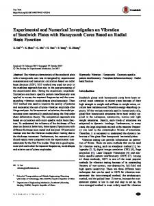
p is the static pressure and τij is the stress tensor. The standard k turbulence model is used to simulate turbulence flow. The standard k model is a semi-empirical model that was introduced by Launder and Spalding (1972). As it can be seen in Fig. 1, the outlet airflow of the Bladeless fan is similar to a free jet flow. Therefore, regarding reasonable precision of the turbulence model to calculate the free jet flow noise, this model was applied in this study. The turbulence kinetic energy, k , and its rate of dissipation, , are described by the following equations:
2. BLADELESS FAN DESCRIPTION Passing air through a Bladeless fan has been illustrated in Fig.1. Surrounding air is sucked into the fan by rotation of radial impellers driven via a DC motor. Afterwards, the air is passed through an annular section and exited from a narrow ring-shape zone. The area reduction at the exit side increases the outlet velocity of airflow. Difference between the air velocity upstream and downstream of the fan leads to a pressure gradient according to Bernoulli equation. This created pressure gradient sucks the air from the back of the fan (upstream) towards the front side (downstream). The outlet flow of the fan includes the inlet flow (passed through the impeller), sucked flow from the upstream which passes through the annular part, plus surrounding airflow. So, total output flow rate measured at a distance of 3D (D is fan diameter) downstream is several times of the inlet flow rate (Gammack et al. 2009). All above steps are depicted in Fig.1.
k ui k x t t x i i k G Y k
M
S
C
1
k
G
k
C
2
(3)
x i
(4)
k
ui x t t x i i
k x i
2 k
S
The turbulent viscosity is evaluated as:
t C
k2
(5)
and
u u Gk t j i xi x j
u j xi
(6)
Gk is production rate of turbulence kinetic energy in the Eqs. (3) and (4).Y M represent the contribution of the fluctuating dilatation in compressible turbulence to the overall dissipation rate. Moreover, S and S k
are user-defined
source terms. In these equations, the constant parameters are C1 1.44 , C 2 1.92 , C 0.09 ,
Fig. 1. Schematic of entry and exit airflow through Bladeless Fan.
k 1.0 and 1.3 (Markatos, 1986).
937
M. Jafari et al. /JAFM, Vol. 9, No. 2, pp. 935-944, 2016. In the current study, in order to discretize time dependent terms in the above-mentioned equations, a second order implicit scheme is applied. Furthermore, the second order upwind has been used for convection terms and the central difference scheme for diffusion terms. The SIMPLE algorithm is applied for pressure-velocity coupling and the obtained solutions are based on time step 0.0001.
consists of surface integrals and volume integrals. The contribution of the volume integrals becomes small when the flow is low subsonic, thus in this study, the volume integrals are dropped. Hence,
p( x , t ) pT ( x , t ) pL ( x , t )
Two terms on the right hand side of Eq. (10), pT ,
p L , are the thickness and ,respectively that are given by
3.2Acoustic Field 3.2.1FW-H Integral Method In this work, the far field noise is computed by solving the FW-H equations. The Ffowcs Williams and Hawkings (1969) formulation is the most general form of the Lighthill’s acoustic analogy and it is appropriate for numerical computation of acoustic fields. This formulation is derived directly from the conservation of mass and momentum equations and then the Heaviside function H ( f ) is employed. The FW-H equations are written as the followings: 1 p 2 p a 2o t 2
f 0
1 4 p L ( x , t ) ao
f 0
ou u n n (f ) t n p ij n j u i u n n (f ) x i
oU n rM r ao M r M 3 f 0 r 2 1 M r
(7)
1 ao
terms
dS
(11)
Lr dS 2 r M 1 r
2
dS
Where t r and ao
T ij H (f ) x i x j
U i i
Where, i and n are the surface velocity in the x i direction and normal to the surface. ui and
(u ) o i i
Li pij n j ui (un n )
u n are the velocity component of fluid in the x i direction and normal to the surface. H ( f ) is the Heaviside function, ( f ) is the Dirac delta function and p is the sound pressure at the farfield location. The first and second terms on the right-hand side of Eq. (7) are monopole (thickness) and dipole (loading) source terms, respectively. The monopole source term is the noise produced via fluid displacement by moving walls. The loading or dipole source term is the influence of unsteady motion of the force distribution on the surface of rigid body. These two source terms are surface ones .The third source term in the Eq. (7) is a quadrupole source term that occurs due to the flow structure. In the Eq. (8), the compressive stress tensor, Pij , and
(12) (13)
Various subscriptions in the Eq. (12) are the inner products of a vector or a unit vector. For example, (14) Lr L r Li ri
Un U n Ui ni
(15)
Where n and r indicate the unit vectors in the wall normal and the radiation directions, respectively. Also the dot operator indicates sourcetime differentiation. The presented formulation is based on the Farassat’s formulation (Farassat et al.(1983)) to solve the FW-H equations.
4.
the Lighthill’s stress tensor, T ij , are defined as follow:
NUMERICALSIMULATION
Based on obtained studies on cross section of this fan by Jafari et al. (2015), Eppler 473 airfoil profile was chosen for the cross section design. An illustration of the designed cross section and its dimensions have been shown in Fig. 2based on Eppler 473. Designed dimensions are 6mm for the outlet slit, 20cm for the length of cross section, and 4.5cm for height of cross section.
(8)
and
Tij ui u j pij a 2o ( 0 ) ij
f 0
L r rM r ao M r M 3 f 0 r 2 1 M r
2
u u 2 uk ij pij p ij i j x j xi 3 xk
2
L L M dS 2 r 2 r 1 M r
loading
o U n U n dS 2 r 1 M r
4 pT ( x , t )
2
(10)
In order to simulate 3D airflow passing through the Bladeless fan, a fan with diameter of 60cm was designed to be in center of a 4.2×4.2×8.4m cubic. The modeled fan in the cubic can be seen in Fig. 3a. In the present study, the motor and impeller section of fan (lower part) were not simulated directly,
(9)
The free-stream quantities in the mentioned equations are specified by the subscript 0. The Eq. (7) is solved utilizing the free-space Green function ( (g )/4 r ). The complete solution of this equation 938
M Jafari et al. /J M. JAFM, Vol. 9, No. N 2, pp. 935-944, 2016. 50L/s inlet flow at 500cm downstream m for three grid cells. It can be found from the curvess in Fig. 4 that the grrid with 24451169 cells is suuitable for the presen nt study. This grid was chhosen for all simulaations of this ressearch.
bbecause incremeent in the output airflow in Bladeeless f fans is due to sppecial geometry of its upper partt. So i was avoided it d to model thee impeller and the c conditions afterr impeller werre applied as inlet b boundary condittions. As it can be seen in Fig. 3a, t air is enterinng the fan from a cylindrical secction the w with a diameterr of 16cm. No slip condition with z zero velocity waas applied to thee floor and the walls w o fan (colored in blue). Constaant relative presssure of b boundary condition was applied a to oother s surrounding wallls.
Fig. 2. Deesigned cross secction of the fan. To calculate thee generated noiise of the Bladeeless T f fan, the output slit was choseen as the source of s sound generation due to decrem ment of thicknesss at t this zone (Jafaari et al. (201 14)), it causes the m maximum veloccity and pressuree fluctuations. Inn the o obtained numerrical simulationn, a sound receeiver w placed in 1m distance from was m the front of faan to c capture the sounnd pressure levvel. Location off this r receiver (R1) is shown in Fig. 3bb.
Fig.44. Velocity proffile at 50cm dow wnstream for flow rate r of 50L/s.
4.2. Acoustic Cod de Validation Produced sound of a NACA 0012 airfoil was mulations and solving s FW-H, calculated by 2D sim mass conservatioon equations. momeentum, and m Bounddary conditions, cell grid, and soome simulation domaiin dimensions are shown in Fig. 5. The adjaceent walls were set in a distance of 10 times of the airrfoil cord to reduce their effecct on the flow aroundd the airfoil (E Eleni et al. 20112). Generated sound was measured by a sound receeiver in a 1.25 m disstance from thhe airfoil trailiing edge. By applyiing an FFT algorrithm, SPL diaggram of NACA 0012 airfoil was calcculated at Re=22×105 and was compaared with Brookks et al. (2012)) experimental data (Fig. 6). The comparison sh hows that the s pressure numerrical simulation can predict the sound level in various freqquencies; howev ver, maximum a frequencies arround 1000 Hz deviattion was found at whichh came with thhe maximum soound level. In additioon, trend of the numerical resultts followed the experiimental data w well. Hence, FW W-H equations were used u to calculatte Bladeless fann sound in the currennt study.
( (a)
( (b)
F 3. a) 3D moodeling of the faan in a cubic rooom, Fig. b)Soound receiver loocation.
4 4.1.Grid Indep pendency Grid study is essential to acquuire a sufficient cell G g grid. Three grids were generaated with 18422679, 2 2445169, and 3265174 3 cell nuumbers in ordeer to c carry out a 3D simulation of thhe fan. Fig. 4 iss the i illustration of thhe exit velocity profile p of the fann for
Fig. 5. 2D modelingg, boundary con nditions, and m mesh generation n for NACA 00112 airfoil.
939
M. Jafarri et al. /JAFM, Vol. 9, No. 2, ppp. 935-944, 20166. hown in Fig. 7bb. The geometry of this Upstream is sh fan in this section is in such a way that t it strengthens Coanda C Effect, w which leads to suction s increment. A wind tunnel inn Sharif University of Technology was w used to carryy out the experimental tests. In the current study, sucked fl flow from the uppstream and total airflow at downstreaam were measu ured. In addition, the experimental e datta were compareed with the numericaal results. For running experimental tests, the inlett section of the fan was conneccted to the outlet of the wind tunnell by a 16cm diameter circle duct. Acccording to Fig. 8a, to measure sucked s flow from the upstream, a cyliindrical channel with a D diameter annd 10D length was connected to the outlet of the fan. This chaannel caused thhe exit airflow structture to a more uniform flow. It was also used to measure m the exit flow at distancee of 8D far from the faan outlet.
6 Comparison of o experimentall data and Fig. 6. numerrical results of produced p sound d by NACA 0012 2 airfoil.
The connectioon of the fan annd the wind tunnnel has been illustrateed in Fig. 8a. A As it can be seeen, for calculating thee sucked flow fr from the upstream m, two pitot tubes weere measured booth dynamic annd total pressures. Too achieve flow increment curv ve, the output airflow w was measuredd simultaneously y with the inlet flow rate into the faan created by thee wind tunnel. Since average veloccity was necesssary to f rate, velocity was averageed over calculate the flow various meaasured points. It is also worth mentioning thhat all measurem ment methods aree based on the AMCA A 210 standard (11999).
5. EXPERIME ENTAL SETU UP Multiplyying the inlet aiirflow is one off the unique characteeristics of Bladeeless fans. To capture the flow inccrement curve of o this fan, a Bladeless B fan with 600cm diameter and a 6mm outpput slit was construccted and tested experimentally. Additionally, A it is worrth mentioning thhat all dimension ns of this fan (experim mental model) were w chosen accoording to the simulateed fan in the preevious section. The T fan was made off 1mm galvanizeed sheet, as it caan be seen in Fig. 7a.
(a)
(b) Fig. 8. a) Illu ustration of the experimental setup, s b) Illustratiiondepictingpitoot tubes No. 1 and a 2 locationss. Pitot tubes loocation before and after the fan f for measuring pressure p is shown in Fig. 8b schematically. As it can be b seen, pitot No. 1 measured the inlet pressure annd No. 2 measurred the outlet pressurre. Location off the pitot No. 2 was three times off the fan diameteer further from the t fan to record flow w rate. The ambbient temperaturre was 27 ºC and the air density was 1.204 kg/m3. PDynamic
d Bladeless fan with w 60cm Fig. 7. a) Constructed meter.b) Backsid de of the fan (up pstream). diam 940
1 V 2 2
(16)
M. Jafari et al. /JAFM, Vol. 9, No. 2, pp. 935-944, 2016. Equation 16 states the relationship between dynamic pressure and instance velocity, so it was used to calculate the air velocity from measured dynamic pressures in each point. Then, the volume flow rate was obtained by multiplying the velocity in cross section area. The comparison of calculated volume flow rates at the inlet and outlet of the fan are shown in Table 1. According to the experiment data, the figure 9 shows the variations of total pressure while the inlet flow rate of fan increases. As shown in Fig.9, the total pressure goes up with increasing of flow rate in the inlet section.
at inlet and outlet of the fan. Table 2 indicates the volume flow rates at inlet and outlet of the fan 3D distance from downstream based on the measured experimental data. Table 2 Flow rate entered into the fan and exited from rectangular channel.
Table 1 Inlet & outlet flow rates through the fan Test
Test-1 Test-2 Test-3 Test-4 Test-5
Inlet Volume Flow rate (m3/s) 0.12 0.136 0.15 0.17 0.195
Outlet Volume Flow rate (m3/s)
Test
Inlet Volume Flow rate (m3/s)
Outlet Volume Flow rate (m3/s)
Test-1 Test-2 Test-3 Test-4 Test-5
0.12 0.136 0.15 0.17 0.195
1.14 1.3 1.43 1.63 1.87
6.
0.86 0.979 0.108 1.224 1.404
RESULTS AND DISCUSSION
Experimental and numerical results have been illustrated here. As it was previously described, a Bladeless fan with a diameter of 60cm and 6mm outlet split was constructed in this study. The thickness of outlet slit had extreme effect in the exit airflow rate, as the less outlet slit thickness, the more output flow velocity. So according to Bernoulli equation, increasing the velocity of exit flow leaded to the increment of pressure gradient between back and front side of the fan. This caused more air suction from upstream. Fig. 11 and 12 show velocity field contour and velocity vectors, respectively. As it is shown, the velocity field around the fan is not symmetric. The velocity at the top of the fan is more than the bottom. Fig. 4 simply confirms linear behavior of velocity profile. Velocity vectors of Fig. 12 show that the specific geometry of fan and its Coanda surface sucks the air from the back forward the front of the fan. Simultaneously, the surrounding air moved forward along with the flow exiting from the fan. Therefore, the total exit flow reached to multiple times of the inlet flow. This is one of the unique characteristics of the Bladeless fans.
Fig. 9. Experimental performance curve of the fan.
In the second step, the fan was put in a channel with cross section of 6D×6D and length of 10D. Afterwards, the total output airflow rate in a distance of three times of the fan diameter downstream was measured (Fig. 10).
Fig. 10. Output flow measurement scheme.
Fig. 11. Velocity contour in the middle section of fan.
Pitot tubes No.1 and 2 measured air pressure (according to Fig. 10) and were used to calculate average velocity, which leaded to volume flow rates
As previously mentioned, a cylindrical channel and a cubic channel were used to measure total exit flow of the fan at 180cm downstream. Experimental and 941
M. Jafari et al. /JAFM, Vol. 9, No. 2, pp. 935-944, 2016. numerical results of the flow increment for the constructed fan were compared in Fig. 13. The curves of Exp. Results-1 and Numerical-1 show sucked flow rate from the upstream and do not include the sucked flow from surrounding zones. The curves of Exp. Results-2 and Numerical-2 show sucked flow rate from both back and surrounding zones. As it can be seen, the diagram of outlet volume flow rate versus inlet volume flow (flow increase curve) shows nearly linear behavior. The proportion of outlet to inlet volume flow rate is equal to the flow increment coefficient of the Bladeless fan. According to Fig. 13, the value of this coefficient for experimental results (Exp. Results-1) and numerical results (Numerical-1) are 7.2 and 8.3, respectively. Therefore, deviation between the experiment and numerical results is around 15%. A portion of this error is rising from numerical errors of solving governing equations and another portion related to errors of the measurement instruments that measured the velocity and pressure field like pitot tubes. In addition, there was some leakage at fasteners because the output airflow from wind tunnel had high pressure. In addition, another parts of errors come from the difference between the numerical modeling and original sections in experiment such as a little difference of fan’s cross section (airfoil shape) in numerical design and prototype fan. Fig. 13shows a deviation between experimental and numerical results of Exp. Results2 and Numerical-2 curves around 13.5%. Obtained values of flow increment coefficient show that the outlet flow in downstream is formed of 8.5% of the inlet flow, 53% of the sucked flow from upstream, and 38.5% of surrounding airflow.
Fig. 13. Comparison of experimental and numerical results of flow increase curve for fan.
To predict the aeroacoustic performance in various conditions FW-H equations were solved in unsteady form. SPL (sound pressure level) and OASPL (overall sound pressure level) diagrams for this fan were captured. Equation 17 was used to calculate the SPL diagram. FFT algorithm was also applied to obtain Fig. 14 curve.
SPL 10log( p / p ref )2
(17)
Which Pref=20×10-6pa.The OASPL term is defined as the Eq. (18). N
OA SPL 10log 10 10(SPLi )/10
(18)
i 1
In Fig. 14, produced frequency spectrum curve of the fan is shown for frequencies between 0 to 5000Hz. As it can be seen, generated sound by the fan covered a wide and broadband frequency range, which reached to higher values at lower frequencies. In addition, this diagram shows that the frequency curve of fan for frequencies between 2500 to 5000Hz is almost flat.
Fig. 12. Velocity vectors of the exit flow for inlet flow rateof 50L/s.
It should be considered that the less thickness of the outlet slit means the more flow increase coefficient. In order to design outlet slit thickness, a few parameters such as manufacturing capability and air velocity at the narrow outlet slit should be taken into account. Since, the Mach number will become near critical amount (M=1) if the inlet flow rate increase while the outlet slit is constant.
Fig. 14. SPL curve for inlet flow rate 50L/s.
For better understanding of the emitted sound from the fan, OASPL diagram was plotted versus various inlet volume flow rates in Fig. 15. The curve 942
M. Jafari et al. /JAFM, Vol. 9, No. 2, pp. 935-944, 2016. indicates that the produced sound increases by increment of the inlet flow rate. Since raising the inlet flow rate increases the velocity of outlet airflow, pressure field fluctuation increases. Increment in the pressure field fluctuation also leads to more produced sound by the fan. The obtained sound results were approximated by
such as underground tunnels or for removing smoke and dust from industrial environments. REFERENCES
AMCA, B. (1999). 210-Laboratory Methods of Testing Fans for Aerodynamic Performance Rating. Air Movement and Control Association International, Inc.
axbformulation, which can be seen in Fig. 15. The approximated equation is as below which IVF is the inlet flow rate in liter per second:
OASPL (dB ) 28.221 IVF ( L / s )
0.1657
Ballesteros-Tajadura, R., S. Velarde-Suárez and J. Hurtado-Cruz (2008).Noise Prediction of a Centrifugal Fan: Numerical Results and Experimental Validation.J. Fluids Eng. 130(9), 091102-091102-12.
(19)
Belkheir, N., R. Dizene and S. Khelladi (2012). A Numerical Simulation of Turbulence Flow Around a Blade Profile of HAWT Rotor in Moving Pulse. Journal of Applied Fluid Mechanics, 5(1), 1-9. Brentner, K. and F. Farassat (1997).An Analytical Comparison of the Acoustic Analogy and Kirchhoff Formulation for Moving Surfaces.In Annual Forum Proceedings-American Helicopter Society 53, 687-696. American Helicopter Society. Brooks, T. F., D. S. Pope and M. A. Marcolini (1989). Airfoil Self-Noise and Prediction. NASA Reference, Publication 1218.
Fig. 15. OASPL curve for Bladeless fan.
7.
Chong, T. P., P. F. Joseph and M. J. Kingan (2012).An Investigation of Airfoil Tonal Noise at Different Reynolds Numbers and Angles of Attack.Applied Acoustics.74, 38–48.
CONCLUSION
In the current study, performance of a Bladeless fan with a 60cm diameter was investigated via both experimental and numerical approaches. The numerical simulation included a cubic room with the modeled fan inside it. Conservative equations of mass and momentum were also used to solve the flow field. Furthermore, FW-H formulation was applied to calculate produced sound of this fan. To validate numerical results of the acoustic code, sound generation of a NACA 0012 airfoil with zero angle of attack and Reynolds number of 2×10⁵ was calculated and compared with the experiments. In the present research, sucked flow rate from back and surrounding zones of the fan were measured and compared with the numerical results. Experimental and numerical results only for sucking from back of the fan showed that flow increase coefficient by experimental and numerical approaches were 7.2 and 8.3 respectively, which were acceptably close to each other. Additionally, other measurements indicated that with considering sucked surround air, flow increase coefficient for experimental results was 11.7 and this value for numerical results was 13.5. The results demonstrated that the outlet flow includes 8.5% inlet airflow, 53% sucked air from upstream, and 38.5% surrounding air. Numerical results of sound prediction showed that increment of the inlet volume flow rate increases produced sound, because of growth of pressure fluctuations at the outlet slit. Finally, results of this research show that Bladeless fan is capable to be designed in large dimensions and be utilized in various industries
Chunxi, L., W. S. Ling and J. Yakui (2011).The Performance of a Centrifugal Fan with Enlarged Impeller.Energy Conversion and Management 52(8), 2902-2910. Cozza, I. F., A. IobandR. Arina (2012). Broadband Trailing-Edge Noise Prediction with a Stochastic Source Model. Computers & Fluids 57, 98-109. Curle, N. (1955). The Influence of Solid Boundaries upon Aerodynamic Sound.Proceedings of the Royal Society of London. Series A. Mathematical and Physical Sciences 231(1187), 505-514. Eleni, D. C., T. I. Athanasios andM. P. Dionissios (2012). Evaluation of the Turbulence Models for the Simulation of the Flow over a National Advisory Committee for Aeronautics (NACA) 0012 Airfoil. Journal of Mechanical Engineering Research 4(3), 100-111. Farassat, F. and G. P.Succi (1983). The Prediction of Helicopter Rotor Discrete Frequency Noise.Vertica7(4), 309-320. Gammack, P.D., F. Nicolas andK. J. Simmonds(2009). Bladeless Fan, in Patent Application Publication. Ghassemi, H. andA. R. Kohansal (2013). Wave Generated by the NACA4412 Hydrofoil 943
M. Jafari et al. /JAFM, Vol. 9, No. 2, pp. 935-944, 2016. NearFree Surface. Journal of Applied Fluid Mechanics 6(1), 1-6.
Science 33(4), 683-694. Lin, S. C. andC. L. Huang (2002).An Integrated Experimental and Numerical Study of Forward– Curved Centrifugal Fan.Experimental Thermal and Fluid Science 26(5), 421-434.
Hotchkiss, P. J., C. J. Meyer andT. W. Von Backström (2006). Numerical Investigation into the Effect of Cross-Flow on the Performance of Axial Flow Fans in Forced Draught Air-Cooled Heat Exchangers. Applied Thermal Engineering 26(2), 200-208.
Maaloum, A., S. KouidriandR. Rey (2004).Aeroacoustic Performance Evaluation of Axial Flow Fans Based on the Unsteady Pressure Field on the Blade Surface.Applied Acoustics 65(4), 367-384.
Ikeda, T., T. AtobeandS. Takagi (2012). Direct Simulations of Trailing-Edge Noise Generation from Two-Dimensional Airfoils at Low Reynolds Numbers. Journal of Sound and Vibration 331(3), 556-574.
Markatos, N. C. (1986). The Mathematical Modelling of Turbulent Fows.Applied Mathematical Modelling 10(3), 190-220.
Jafari, M., H. Afshin, B. Farhanieh andH. Bozorgasareh (2015). Numerical Aerodynamic Evaluation and Noise Investigation of a Bladeless Fan.Journal of Applied Fluid Mechanics8(1), 133-142.
Mathey, F. (2008). Aerodynamic Noise Simulation of the Flow Past an Airfoil Trailing-Edge Using a Hybrid Zonal RANS-LES. Computers & Fluids 37(7), 836-843.
Jeon, W. H., S. J. BaekandC. J. Kim (2003).Analysis of the Aeroacoustic Characteristics of the Centrifugal Fan in a Vacuum Cleaner.Journal of Sound and Vibration 268(5), 1025-1035.
Tannoury, E., S. Khelladi, B.Demory, M. HennerandF. Bakir (2013).Influence of Blade Compactness and Segmentation Strategy on Tonal Noise Prediction of an Automotive Engine Cooling Fan.Applied Acoustics 74(5), 782-787.
Kergourlay, G., S. Kouidri, G. W. Rankin, R. Rey (2006). Experimental Investigation of the 3D Unsteady Flow Field Downstream of Axial Fans. Flow Measurement and Instrumentation 17(5), 303-314.
Thiart, G. D. andT. W. Von Backström (1993). Numerical Simulation of the Flow Field Near an Axial Flow Fan Operating under Distorted Inflow Conditions. Journal of Wind Engineering and Industrial Aerodynamics 45(2), 189-214.
Khelladi, S., S. Kouidri, F. BakirandR. Rey (2008).Predicting Tonal Noise from a High Rotational Speed Centrifugal Fan.Journal of Sound and Vibration 313(1), 113-133.
Williams, J. F. andD. L. Hawkings (1969). Sound Generation by Turbulence and Surfaces in Arbitrary Motion. Philosophical Transactions of the Royal Society of London. Series A, Mathematical and Physical Sciences 264(1151), 321-342.
Launder, B. E. andD. B. Spalding (1972). Mathematical Models of Turbulence. Academic Press ,London.
Zhou, Q. andP. Joseph (2007).A Frequency Domain Numerical Method for Airfoil Broadband SelfNoise Prediction.Journal of Sound and Vibration 299(3), 504-519.
Li, H. (2009). Flow Driven by a Stamped Metal Cooling Fan–Numerical Model and Validation.Experimental Thermal and Fluid
944